the Creative Commons Attribution 4.0 License.
the Creative Commons Attribution 4.0 License.
 | 13 Nov 2018
Tropospheric ozone in CCMI models and Gaussian process emulation to understand biases in the SOCOLv3 chemistry–climate model
Laura E. Revell
Andrea Stenke
Fiona Tummon
Aryeh Feinberg
Eugene Rozanov
Thomas Peter
N. Luke Abraham
Hideharu Akiyoshi
Alexander T. Archibald
Neal Butchart
Makoto Deushi
Patrick Jöckel
Douglas Kinnison
Martine Michou
Olaf Morgenstern
Fiona M. O'Connor
Luke D. Oman
Giovanni Pitari
David A. Plummer
Robyn Schofield
Kane Stone
Simone Tilmes
Daniele Visioni
Yousuke Yamashita
Guang Zeng
Previous multi-model intercomparisons have shown that chemistry–climate models exhibit significant biases in tropospheric ozone compared with observations. We investigate annual-mean tropospheric column ozone in 15 models participating in the SPARC–IGAC (Stratosphere–troposphere Processes And their Role in Climate–International Global Atmospheric Chemistry) Chemistry-Climate Model Initiative (CCMI). These models exhibit a positive bias, on average, of up to 40 %–50 % in the Northern Hemisphere compared with observations derived from the Ozone Monitoring Instrument and Microwave Limb Sounder (OMI/MLS), and a negative bias of up to ∼30 % in the Southern Hemisphere. SOCOLv3.0 (version 3 of the Solar-Climate Ozone Links CCM), which participated in CCMI, simulates global-mean tropospheric ozone columns of 40.2 DU – approximately 33 % larger than the CCMI multi-model mean. Here we introduce an updated version of SOCOLv3.0, “SOCOLv3.1”, which includes an improved treatment of ozone sink processes, and results in a reduction in the tropospheric column ozone bias of up to 8 DU, mostly due to the inclusion of N2O5 hydrolysis on tropospheric aerosols. As a result of these developments, tropospheric column ozone amounts simulated by SOCOLv3.1 are comparable with several other CCMI models. We apply Gaussian process emulation and sensitivity analysis to understand the remaining ozone bias in SOCOLv3.1. This shows that ozone precursors (nitrogen oxides (NOx), carbon monoxide, methane and other volatile organic compounds, VOCs) are responsible for more than 90 % of the variance in tropospheric ozone. However, it may not be the emissions inventories themselves that result in the bias, but how the emissions are handled in SOCOLv3.1, and we discuss this in the wider context of the other CCMI models. Given that the emissions data set to be used for phase 6 of the Coupled Model Intercomparison Project includes approximately 20 % more NOx than the data set used for CCMI, further work is urgently needed to address the challenges of simulating sub-grid processes of importance to tropospheric ozone in the current generation of chemistry–climate models.
- Article
(3826 KB) -
Supplement
(836 KB) - BibTeX
- EndNote


Ozone is a key trace gas in the atmosphere. In the stratosphere, it absorbs UV-B ( nm) radiation and thus protects life at the surface. However in the troposphere, where approximately 10 % of the total atmospheric ozone burden resides, ozone is a greenhouse gas and air pollutant, with adverse affects on human health and crop yields (Myhre et al., 2013; Silva et al., 2013, 2017; Stevenson et al., 2013). Approximately 90 % of tropospheric ozone results from a series of photochemical reactions which are initiated by the reaction of NOx (nitrogen oxides, NOx = NO+NO2) and either CO (carbon monoxide), CH4 (methane) or an NMVOC (non-methane volatile organic compound) (Denman et al., 2007). These ozone precursors are emitted from, amongst other sources, fossil fuel burning, industrial processes and agriculture. Ozone can also be transported from the stratosphere in stratosphere–troposphere exchange (STE) events. Greenslade et al. (2017) calculate the mean fraction of total tropospheric ozone attributable to STE at three sites between 38 and 69∘ S as 1 %–3 %, and show that during individual STE events, over 10 % of tropospheric ozone may be directly transported from the stratosphere. Due to its global tropospheric lifetime of ∼22 days, ozone is subject to intercontinental transport (Auvray and Bey, 2005), and this is modulated by decadal climate variability (Lin et al., 2014). Ozone is lost from the troposphere either by dry deposition or photochemical destruction.
Most chemistry–climate models (CCMs), which are used to understand chemistry–climate interactions and project future atmospheric composition, overestimate tropospheric ozone in the Northern Hemisphere compared with observations (Parrish et al., 2014; Young et al., 2013, 2018). In particular, version 3.0 of the SOCOL (Solar-Climate Ozone Links) CCM (Sect. 2.2) contains notable positive tropospheric ozone biases. Revell et al. (2015) identified that ozone concentrations in SOCOLv3.0 are up to 50 % too high in the Northern Hemisphere mid-troposphere (500 hPa) compared with observations from the Tropospheric Emission Spectrometer (TES). The reasons underlying SOCOLv3.0's tropospheric ozone bias were not completely clear to Revell et al. (2015), who noted that, while SOCOLv3.0 could accurately simulate the general geographic distribution of tropospheric ozone, the actual magnitude was wrong and likely to be “a source issue (that is, emissions), a sink issue (HNO3 washout), or a combination of the two.”
Staehelin et al. (2017) showed that the mean tropospheric ozone burden in SOCOLv3.0 is 413 Tg, which is approximately 80 Tg larger than the multi-model mean burdens reported for the ACCENT (Atmospheric Composition Change: the European Network of Excellence; Stevenson et al., 2006) and ACCMIP (Atmospheric Chemistry and Climate Model Intercomparison Project; Young et al., 2013) activities, of 337 and 336 Tg, respectively. Furthermore, SOCOLv3.0 overestimates both the tropospheric ozone production and destruction rates compared to the multi-model means from ACCENT and ACCMIP (Staehelin et al., 2017). While SOCOLv3.0's production rates are overestimated by 34 % compared to ACCENT and 41 % compared to ACCMIP, the destruction rates are overestimated only by 20 % (ACCENT) and 31 % (ACCMIP).
Recently a newer version of SOCOL has been developed, “SOCOLv3.1”, which remediates obvious deficiencies in SOCOLv3.0's representation of tropospheric processes (Sect. 2.3). We compare tropospheric column ozone in SOCOLv3.0 and 3.1 with observations derived from OMI/MLS, the Ozone Monitoring Instrument/Microwave Limb Sounder (Sect. 3.1), and use Gaussian process (GP) emulation and sensitivity analysis to investigate the remaining ozone bias in SOCOLv3.1 (Sect. 3.2). Because thousands of simulations are required to perform a sensitivity analysis, and this would be computationally inefficient with a CCM, we supplement SOCOLv3.1 with a GP emulator. This allows a sensitivity analysis to be performed at low computational cost. Variance-based sensitivity analysis evaluates a suite of model input parameters and their relationship to the variable of interest simultaneously.
Here, we apply GP emulation and variance-based sensitivity analysis to the SOCOLv3.1 tropospheric ozone budget to understand causes of the bias. In contrast to one-at-a-time testing, which investigates the model response to varying one input parameter while holding all others constant, GP emulation allows all parameters to be evaluated simultaneously and covers more of the parametric uncertainty space than one-at-a-time testing. GP emulation is computationally efficient and allows the interacting effects of the uncertainties on different input parameters to be accounted for. It also generates much more information than one-at-a-time testing – typically the same level of information as a Monte Carlo approach, but requiring a fraction of the model simulations (O'Hagan, 2006). GP emulation has only been used by the global atmospheric modelling community in the last few years, in applications such as cloud and aerosol microphysics modelling (Carslaw et al., 2013; Johnson et al., 2015; Lee et al., 2011, 2012) and chemical transport modelling (Ryan et al., 2018). This is the first time the technique has been applied to global tropospheric ozone. Our GP emulator experiments have been designed to focus on recent developments regarding SOCOL's tropospheric chemistry scheme; however the methodology has the potential to be expanded to also include meteorological parameters.
SOCOLv3.0 participated in phase 1 of the Chemistry-Climate Model Initiative (CCMI) (Eyring et al., 2013b; Morgenstern et al., 2017), which is a joint activity of SPARC (Stratosphere–troposphere Processes And their Role in Climate) and IGAC (International Global Atmospheric Chemistry), and is the successor activity to phase 2 of the Chemistry-Climate Model Validation activity, CCMVal-2 (SPARC CCMVal, 2010). Unlike CCMVal-2, which focussed on stratospheric processes and composition, CCMI includes many models with comprehensive representations of the troposphere, and aims to additionally address aspects of tropospheric chemistry and circulation. Here, we examine tropospheric column ozone in SOCOLv3.0 and 14 other CCMI models. This is the first time that global distributions of tropospheric ozone have been examined in the CCMI models, and results are presented in Sect. 3.3.
2.1 CCM simulations to compare with observations
We use the ensemble mean of three free-running SOCOLv3.0 simulations of the recent past to compare with observations (ETH-PMOD, 2015). These simulations were performed for CCMI, and conform to REF-C1 specifications (Eyring et al., 2013b). The simulations cover the period 1960–2010, following a 10-year spin-up period. Greenhouse gas concentrations (CH4, CO2 and N2O) follow observations until 2005, then Representative Concentration Pathway (RCP) 8.5 (Riahi et al., 2011). Ozone precursor emissions (including NOx, CO and NMVOCs) follow a historical emissions inventory until 2000 (Lamarque et al., 2010), then RCP 6.0 (Masui et al., 2011). Sea surface temperatures (SSTs) and sea ice concentrations were prescribed following HadISST observations (Rayner et al., 2003). Concentrations of ozone-depleting substances followed the World Meteorological Organization's A1 scenario (WMO, 2011), and stratospheric aerosol surface area densities and optical parameters were prescribed from the SAGE-4λ data set (Arfeuille et al., 2013; Luo, 2013).
We also examine annual-mean tropospheric ozone in REF-C1 simulations performed by models participating in CCMI, described by Morgenstern et al. (2017) and references therein. Using the simulated ozone volume mixing ratio and WMO-defined tropopause height from each model, tropospheric ozone columns were calculated for the year 2005 by integrating ozone between the surface and WMO-defined tropopause. The WMO definition of the tropopause was selected to be consistent with the OMI/MLS tropospheric ozone product (Ziemke et al., 2006). Between 2010 and 2014, the average tropospheric ozone burden derived from OMI/MLS was 300 Tg, which is very close to the multi-instrument mean of five satellite products over the same period, of 301 Tg (Gaudel et al., 2018).
Where multiple ensemble members (“realizations”) of the REF-C1 simulation were submitted to the CCMI archive, the ensemble mean is shown. The exception is NIWA-UKCA, which submitted three realizations of the REF-C1 simulation; however only the first realization is shown as ozone precursor emissions were erroneously fixed at 1960 levels for the other two realizations (Morgenstern et al., 2017). The EMAC simulations used road traffic emissions which were updated every year rather than every month. Therefore when we examine year 2005 tropospheric column ozone in Sect. 3.3, the EMAC simulations used road traffic emissions for August 1954. Jöckel et al. (2016) show that this error results in tropospheric ozone columns that are ∼2 DU lower than if the correct emissions had been used. The UMUKCA-UCAM simulations used CCMVal-2 REF-B2 emissions for NOx aircraft emissions and NOx, CO and HCHO surface emissions.
2.2 The SOCOLv3.0 chemistry–climate model
The SOCOL CCM was developed in Switzerland at ETH Zurich and PMOD/WRC (the Physical Meteorological Observatory Davos/World Radiation Center). Version 3.0 of SOCOL (Revell et al., 2015; Stenke et al., 2013) consists of the middle atmosphere version of the ECHAM5 (European Centre Hamburg Model) atmosphere-only general circulation model (Roeckner et al., 2003) coupled to the MEZON (Model for Ozone Trends) chemistry transport model (Egorova et al., 2003). The chemical solver takes into account 41 chemical species, 140 gas-phase reactions, 46 photolysis reactions and 16 heterogeneous reactions. The oxidation of isoprene, an important NMVOC for the tropospheric ozone budget, is accounted for with the Mainz Isoprene Mechanism (MIM-1), which comprises 16 organic degradation products of isoprene and a further 44 chemical reactions (Pöschl et al., 2000). Global isoprene emissions are estimated to range from 440 to 660 Tg(C) yr−1, which is comparable to the annual amount of CH4 emissions (Guenther et al., 2006). About two-thirds of the annual global emissions of volatile organic compounds (VOCs) are accounted for in SOCOLv3.0 by isoprene and methane. Apart from isoprene and formaldehyde, other NMVOCs are not included explicitly in the model but their contribution to CO is accounted for via the addition of a certain fraction of NMVOC emissions to CO. For anthropogenic, biomass burning and biogenic NMVOC emissions the conversion factors to CO are 1.0, 0.31 and 0.83, respectively (Ehhalt et al., 2001).
Clear-sky photolysis rates are calculated using a lookup-table (LUT) approach, which provides photolysis rates as a function of overhead ozone and oxygen columns (Rozanov et al., 1999). Variability of solar irradiance is included in the LUTs. Cloud impacts on photolysis are accounted for in the troposphere by the inclusion of a cloud modification factor following the parametrization described by Chang et al. (1987). From a recent intercomparison of photolysis rates simulated by different CCMI models we learned that SOCOLv3.0 overestimates tropospheric NO2 photolysis by roughly a factor of 2 compared to other models (Nicely et al., 2018). This overestimation is likely related to the treatment of backscattering from clouds in the calculations of the photolysis LUTs and the missing impact of aerosols. Both effects cannot be easily corrected by the implemented cloud modification factor, and so an online photolysis scheme is planned for future model versions.
Dry deposition velocities of O3, CO, NO, NO2, HNO3 and H2O2 are based on Hauglustaine et al. (1994). This simplified approach assumes constant dry deposition velocities over land and ocean, without accounting for seasonal or geographical variability. The tropospheric washout of HNO3 and H2O2 is calculated by using a constant removal rate of s−1, irrespective of precipitation occurrence. At every chemical time step, i.e. every 2 h, 2.8 % of tropospheric HNO3 and H2O2 below 160 hPa are removed. Boundary conditions for the ozone precursor gases NOx, CO and NMVOCs are implemented as surface emission fluxes. Methane's global average surface mixing ratio is prescribed on the six lowermost model levels. For this study, both SOCOL configurations were run with 39 vertical levels between the Earth's surface and 0.01 hPa (∼80 km) and T42 horizontal resolution (grid cells approximately 2.8∘ × 2.8∘).
2.3 Upgraded model version SOCOLv3.1
SOCOLv3.1 was developed to address SOCOLv3.0's representation of processes relevant to tropospheric ozone chemistry, with the aim of improving the model's large tropospheric ozone bias as shown by Revell et al. (2015). First, we implemented heterogeneous hydrolysis of N2O5 on tropospheric aerosol, as this is an important removal process for atmospheric NOx and was not included in SOCOLv3.0. As SOCOLv3.0 does not explicitly simulate tropospheric aerosols, the new scheme makes use of the ECHAM5 internal tropospheric aerosol climatology considering aerosol properties of 11 Global Aerosol Data Set types (Köpke et al., 1997). The reaction probabilities for the different aerosol types are calculated following the parametrization by Evans and Jacob (2005).
Second, the simplified treatment of dry deposition was replaced by a more sophisticated scheme in SOCOLv3.1 based on the surface resistance approach for the estimation of dry deposition velocities proposed by Wesely (1989). This takes into account actual meteorological conditions, different surface types and trace gas properties like solubility and reactivity. Further details of this scheme are given by Kerkweg et al. (2006).
Third, we adjusted how methane is prescribed in the model. In previous versions of SOCOL, methane was prescribed as a global surface average mixing ratio on the six lowermost model levels (covering approximately 2.5 km). This was changed to only the surface level in SOCOLv3.1. While the amount of methane entering the atmosphere is the same in both configurations, prescribing it on one level instead of six means that methane-induced ozone production in the mid-troposphere–upper troposphere is reduced. Because SOCOLv3 has a high OH bias compared to the ACCMIP models (Staehelin et al., 2017), ozone production from methane oxidation is amplified by the continuous resupply of methane due to the mixing ratio boundary condition when methane is prescribed on six levels instead of one. An interhemispheric gradient and seasonal cycle in methane have also been implemented in SOCOLv3.1; however these were not used in this study and instead methane was prescribed as a global average surface mixing ratio to test the general sensitivity of tropospheric ozone to surface methane concentrations.
Finally, because the LUTs used in SOCOLv3.0 cause tropospheric NO2 photolysis to be overestimated due to the treatment of backscattering from clouds (Sect. 2.2), we recalculated LUTs for SOCOLv3.1. While the SOCOLv3.0 LUTs were calculated assuming 0.5 cloud coverage and a surface albedo of 0.3, the SOCOLv3.1 LUTs were based on clear-sky conditions and also used a surface albedo of 0.3.
2.4 SOCOLv3.1 simulations for GP emulator training and testing
Variance-based global sensitivity analysis quantifies the contribution of a single parameter to the variance of a model's output. Because the large number of model simulations required would make one-at-a-time testing computationally too expensive, a type of statistical model called a GP emulator can be used as a surrogate for the input–output relation of a complex model, such as a CCM (Le Gratiet et al., 2017). For “training” data on which the GP emulator is built, we know that the true value of the emulated output should be the same as the input, so the emulator should return the output with no uncertainty. For inputs that the emulator is not trained at, the outputs should have a probability distribution specified by a mean function and covariance function (O'Hagan, 2006). Here, we use tropospheric ozone columns from SOCOLv3.1 to train the emulator.
Interacting contributions to the overall uncertainty in tropospheric column ozone can be identified by comparing the main effect variance (the reduction in the ozone variance when a particular model forcing is fixed, e.g. NOx emissions), with the total effect variance (the remaining variance in the tropospheric column ozone when everything except a particular model forcing is fixed). Various software packages are available for GP emulation. We used the Gaussian Emulation Machine for Sensitivity Analysis (GEM-SA), available at http://tonyohagan.co.uk/academic/GEM/index.html (last access: 11 November 2018), to build an emulator for tropospheric column ozone.
Table 1Range of the sensitivity forcings/parametrizations. P and L indicate whether the variable is of relevance to ozone production and/or loss, respectively.
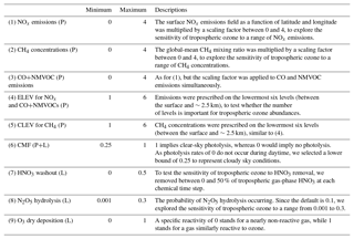
Although many factors influence the tropospheric ozone budget, we restricted our analysis to nine model forcings/parametrizations (see Table 1 for details of the scalings applied). These are listed below, followed by a section rationalizing the inclusion of each variable. We reiterate that this list above does not constitute a comprehensive list of variables controlling tropospheric ozone; however by illustrating the methodology used, we aim to demonstrate its utility.
-
natural and anthropogenic NOx emissions (denoted in figures as “NOx”).
-
methane concentrations (“CH4”);
-
CO emissions (natural and anthropogenic) and NMVOC emissions (anthropogenic, biogenic and biomass burning) (“CO”);
-
the number of vertical levels NOx and CO+NMVOC emissions prescribed on in the model (“ELEV”);
-
the number of vertical levels CH4 concentrations prescribed on in the model (“CLEV”);
-
the impact of clouds on photolysis rates, via the cloud modification factor (“CMF”);
-
the rate of HNO3 washout (“HNO3”);
-
the N2O5 uptake coefficient, which represents the probability of N2O5 hydrolysis occurring (“N2O5”);
-
the specific reactivities for ozone dry deposition (“O3DD”), which are used to estimate the dry deposition velocity.
Variables (1–3) were selected due to their importance as tropospheric ozone precursors. CO and NMVOC emissions were varied simultaneously (3) because the only NMVOCs included explicitly in SOCOL are isoprene and formaldehyde; other NMVOCs are represented via additional CO using a “lumped” approach (Sect. 2.2). For models with a more complex representation of NMVOCs, we recommend testing CO and NMVOC emissions separately when constructing a GP emulator.
The remaining variables were included to investigate the sensitivity of tropospheric ozone to the model improvements implemented in SOCOLv3.1. SOCOLv3.0 and its predecessors prescribed methane on the lowermost six model levels. This was changed to only the surface level in SOCOLv3.1, and variable (5) was included in our analysis to investigate the sensitivity of tropospheric ozone to this implementation. The lowermost level in SOCOL covers approximately 100 m, and the six lowermost levels combined cover approximately 2.5 km. To explore whether other ozone precursors are sensitive to the number of levels they are prescribed on, variable (4) was included, even though it is prescribed only as a surface emissions flux in most, if not all, CCMs. By doing so, we aim to test the exchange of emissions between the boundary layer and free troposphere.
Because ozone production and destruction reactions are mostly photochemical, i.e. they occur in the presence of sunlight, we selected variable (6) to test the sensitivity of the current CMF parametrization, and examine impacts of the updated LUTs on tropospheric ozone in SOCOLv3.1. HNO3 washout is the main sink for NOx, and therefore affects the ozone budget. Future SOCOL versions will include an online wet deposition scheme, and so variable (7) was selected to probe the sensitivity of tropospheric ozone to the rate of HNO3 loss. Heterogeneous N2O5 hydrolysis is similarly important as it leads to HNO3 formation; however it was not included in SOCOLv3.0. Therefore variable (8) was included in our analysis to quantify its relevance for tropospheric ozone abundances. Finally, variable (9) was chosen to test the sensitivity of tropospheric ozone to the newly implemented dry deposition parametrization (Sect. 2.3).
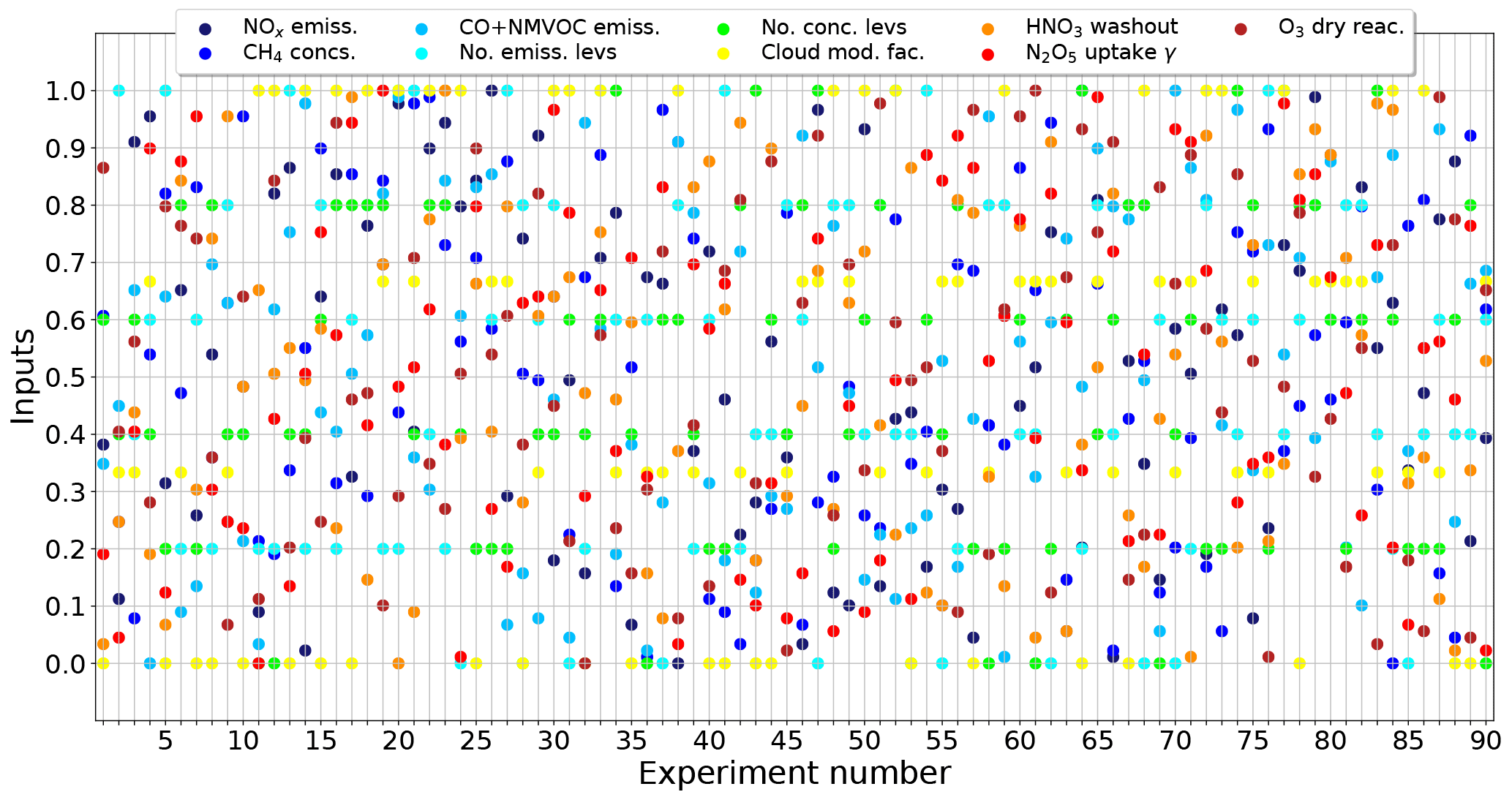
Figure 1Experimental design for the 90 SOCOLv3.1 simulations performed to train the GP emulator. Each column of dots indicates the relative scaling applied to each of the nine variables – see Table 1 for more details. For clarity the inputs have been scaled between 0 and 1.
Typically 10n simulations are recommended for training a GP emulator, where n is the number of variables under investigation (Loeppky et al., 2009). Hence we performed 90 SOCOLv3.1 training simulations, and used the resulting annual-mean tropospheric ozone column to construct the GP emulator in several geographical regions (Europe, United States, Asia, the Southern Ocean and the global mean). For each of the 90 training simulations, the nine input variables were scaled simultaneously, with the scaling factors determined using a “maximin” Latin hypercube design, which generates a near-random sample of parameter values from a multidimensional distribution and fills the uncertainty space of the parameters (McKay et al., 1979). The Latin hypercube was generated using GEM-SA. For the discrete input parameters (e.g. (4) and (5) in the list above), the scaling factor was rounded to the nearest whole number. Table 1 summarizes the minimum and maximum scalings applied to each of the nine variables. This is discussed further in Sect. 3.2. Figure 1 shows the experimental design for the 90 training simulations.
SOCOLv3.1 training simulations were performed for the year 2005 (following a common model spin-up period of 10 years, which was discarded from our analysis). The feedback between chemistry and radiation was switched off to keep internal variability as small as possible. Switching off the chemistry–radiation feedback means that all simulations have the same meteorology (given that they started from the same initial conditions and ran with the same dynamical boundary conditions), despite having different chemistry. Therefore, we can be confident that the differences between the simulations are caused by differences in chemistry and not dynamics.
The emulator was constructed using tropospheric ozone columns calculated between the surface and the WMO-defined tropopause. Alongside the global mean, we focus on four regions, namely Europe (37–60∘ N, 0–42∘ E), the United States (32–52∘ N, 67–124∘ W), Asia (6–49∘ N, 70–146∘ E) and the Southern Ocean (45–60∘ S, all longitudes), where different chemical regimes may dominate; see e.g. Sillman et al. (1990).
After constructing the GP emulator, the next step is to validate it by comparing emulator-predicted ozone with SOCOL-simulated ozone. This was done by performing a further 27 (i.e. 3n) SOCOLv3.1 “test” simulations. The set-up for these simulations was similar to the training simulations, with a new Latin hypercube generated by GEM-SA to supply the scaling factors.
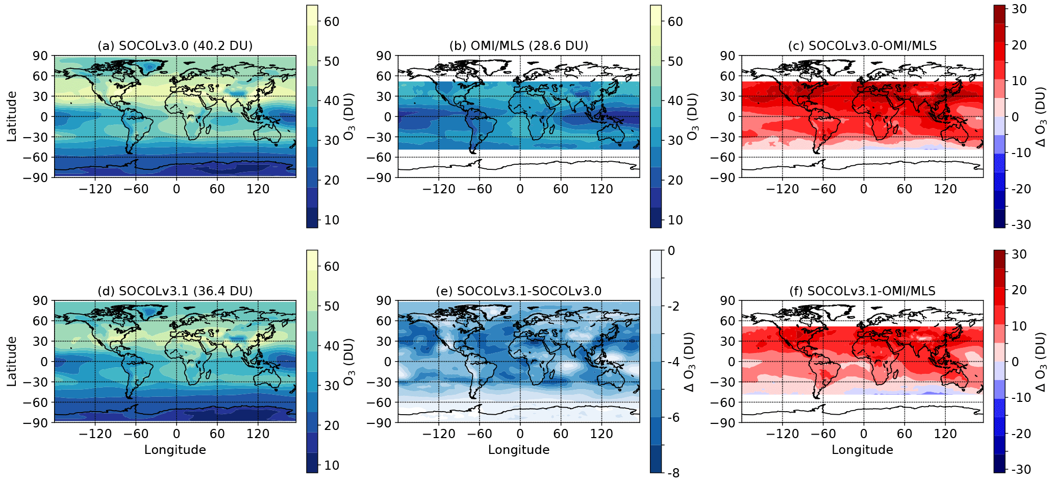
Figure 2Annual-mean year 2005 tropospheric column for (a) SOCOLv3.0; (b) OMI/MLS observations; (c) the difference between SOCOLv3.0 and OMI/MLS; (d) SOCOLv3.1; (e) The difference between SOCOLv3.1 and SOCOLv3.0; (f) the difference between SOCOLv3.1 and OMI/MLS. The global-mean tropospheric column ozone amount is indicated in the title for (a), (b) and (d).
3.1 Tropospheric ozone in SOCOLv3.1
Figure 2 compares annual-mean tropospheric column ozone as simulated by SOCOLv3.0 and 3.1 with observations derived from OMI/MLS. Although SOCOLv3.0 captures the spatial distribution of tropospheric ozone fairly well in a qualitative sense, i.e. elevated ozone in the Northern Hemisphere and a minimum over the tropical Western Pacific (Fig. 2a), it overestimates tropospheric column ozone between 60∘ N and 40∘ S by up to 30 DU – approximately a factor of 2 (Fig. 2c). The improved treatment of ozone sink processes in SOCOLv3.1 means that tropospheric ozone columns are reduced regionally by up to 8 DU compared with SOCOLv3.0 (Fig. 2d–e). Individual sensitivity tests (not shown) indicate that this is due mostly to the inclusion of heterogeneous N2O5 hydrolysis on tropospheric aerosol.
Both SOCOLv3.0 and 3.1 show a small negative bias in tropospheric ozone over the Southern Ocean. This was also visible in the SOCOLv3.0 and TES comparison presented by Revell et al. (2015). Recent work by Luhar et al. (2017) has indicated that the Wesely (1989) dry deposition scheme overestimates the observed ozone deposition velocity by a factor of 2–4 in the Southern Ocean, where SSTs are low and chemical reactions are slow. Further upgrades to the model's deposition scheme may therefore improve comparisons of simulated and observed tropospheric ozone in cold oceanic regions.
The global-mean tropospheric ozone column in SOCOLv3.1 is 36.4 DU (Fig. 2d), which is still at the upper end of the range of the CCMI models (Fig. 6), but comparable to other models such as ACCESS (36.3 DU), EMAC-L47 (37.3 DU) and MRI-ESMr1 (35.7 DU). Despite the improvements to SOCOLv3.1, a large bias in tropospheric ozone of approximately 20 DU compared with OMI/MLS remains (Fig. 2f). The bias maximizes over continental regions in the Northern Hemisphere, and over Southeast Asia.

Figure 3Tropospheric column ozone as predicted by the GP emulator vs. the amount simulated in SOCOLv3.1 test simulations (i.e. the simulations used to validate the emulator). The error bars indicate the uncertainty (mean ± standard deviation) on the GP emulator output, and the 1:1 line and coefficient of determination (R2 value) are also shown. These simulations correspond to running the GP emulator and the simulator (SOCOLv3.1) at each of the 27 validation inputs, for (a) Europe (37–60∘ N, 0–42∘ E); (b) United States (32–52∘ N, 67–124∘ W); (c) Asia (6–49∘ N, 70–146∘ E), (d) the Southern Ocean (45–60∘ S, all longitudes) and (e) globally.
3.2 GP emulation and sensitivity analysis in SOCOLv3.1
To understand the drivers of the remaining tropospheric ozone bias in SOCOLv3.1, we constructed a GP emulator from the 90 SOCOLv3.1 training simulations (Sect. 2.4). Tropospheric ozone predicted by the emulator is compared with SOCOLv3.1 test simulations in Fig. 3. In all geographical regions shown, the goodness of fit between emulated and simulated tropospheric ozone is high (R2≥0.85) and the points fall mostly along the 1:1 line, indicating that the emulator performs well in these regions. The point with the largest simulated tropospheric ozone column corresponds to a simulation in which two ozone loss processes, HNO3 washout and ozone dry deposition, were set to zero and large scalings (4.00 and 3.54) were applied to the ozone precursors NOx and CH4, respectively, following the Latin hypercube design (Fig. 1). The emulator underestimates tropospheric ozone for this point in all regions examined, indicating that it may not be well constrained at the extreme ends of the parameter uncertainty space.
.
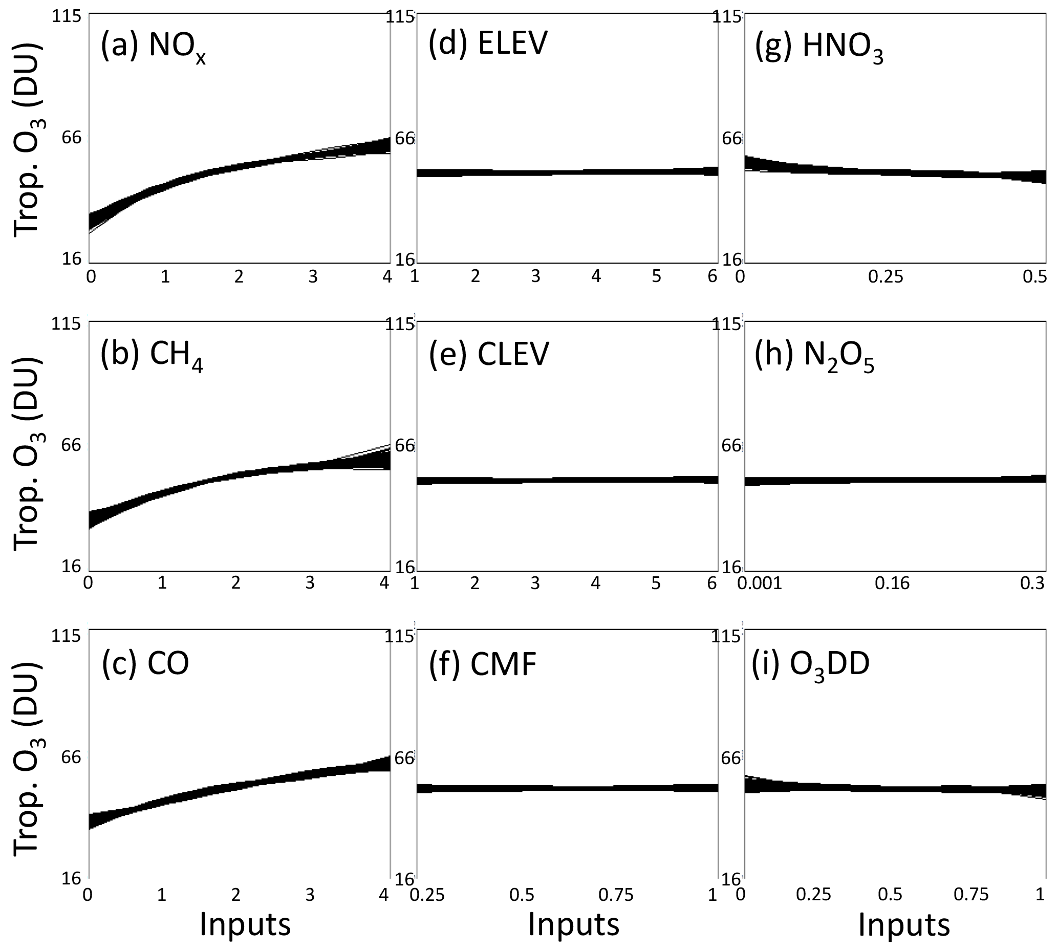
Figure 4Sensitivity of annual global-mean tropospheric column ozone in 2005 to each of the nine sensitivity forcings/parametrizations listed in Table 1, averaging over the other inputs. The horizontal axis shows the range of scaling factors applied to each variable. Plots for individual regions (Europe, the United States, Asia and the Southern Ocean) are in the Supplement.
Figure 4 displays the sensitivity of global-mean tropospheric ozone to each parameter, obtained by averaging over all other parameters, and indicates whether tropospheric ozone increases or decreases in response to an individual forcing/parametrization. Greater uncertainty is indicated where the lines diverge (appearing as a thicker line – i.e. the emulator is less well constrained). Tropospheric ozone exhibits a strong sensitivity to its precursor gases (Fig. 4a–c), and while the correlation between CH4 and CO+NMVOCs is approximately linear, for NOx there appears to be a saturation effect for scaling factors greater than 1, likely due to the “NOx titration effect” (Thornton et al., 2002). In our calculations a uniform sampling distribution was applied when generating the Latin hypercube, which means that in 25 % of our training simulations the NOx (and CH4, CO and NMVOC) scaling factors are less than 1, while in the other 75 % of simulations they are larger than 1.
To test whether the emulator may be biased due to the sampling distribution used, we calculated tropospheric column ozone as a function of NOx and CO+NMVOCs using the gradients in Fig. 4a and c. Assuming a uniform sampling distribution between 0 and 4, as per the Latin hypercube design used here, the sensitivity indices for NOx and CO+NMVOCs are 0.68 and 0.32, respectively. If we assume a piecewise uniform distribution, so that 50 % of the points are between 0 and 1, and 50 % are between 1 and 4, the sensitivity indices are 0.72 for NOx and 0.28 for CO+NMVOCs. That is, the differences are negligible, implying that the type of sampling distribution used does not bias the result. However, given the NOx saturation effect above 1 (Fig. 4a), if we assume a uniform distribution between 0 and 2 instead of 0 and 4, the NOx sensitivity index increases to 0.86, while the CO index decreases to 0.14. This shows the importance of selecting an appropriate range for the parameter uncertainty space. However, the conclusions of our emulator analysis – that ozone precursors are the dominant driver of tropospheric ozone variability – remain unchanged.
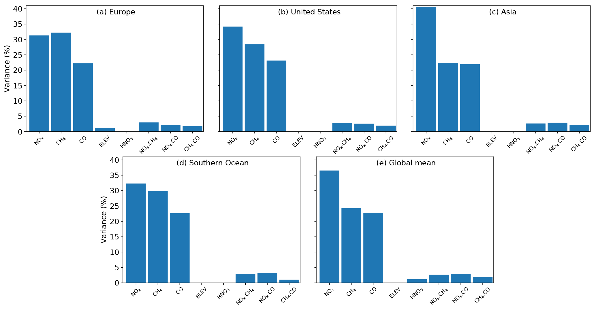
Figure 5Contributions to variance from the sensitivity forcings/parametrizations applied (Table 1), for the same regions shown in Fig. 3. For clarity only those which contribute at least 1 % to the variance are shown. NOx is the NOx emissions; CH4 is the CH4 concentrations; CO is the CO+NMVOC emissions; ELEV is the number of vertical model levels that NOx, CO and NMVOC emissions are prescribed on. HNO3 is the rate of HNO3 washout. Joint interactions, indicated by, e.g. NOx. CH4 concentrations are also indicated where these contribute at least 1 % to the variance.
Figure 5 shows the percentage of variance that each parameter contributes to in each geographic region, either jointly or alone. In all regions examined, ozone precursors – CH4, NOx, CO and NMVOCs – account for more than 90 % of the variance in tropospheric column ozone. In other words, changing these ozone source input parameters has a far larger impact on tropospheric ozone abundances than changing ozone sink parameters does, and this applies to both polluted regions (Europe, the United States and Asia) and relatively pristine environments (the Southern Ocean). NOx emissions are generally the dominant driver of variability (in the European region they are approximately equal to the contribution from CH4; Fig. 5a). Over Asia, where CO emissions are larger than over Europe and the United States, the ratio of NOx:CO is also lower than it is over Europe and the United States (Revell et al., 2015). NOx emissions therefore become more important as a driver of ozone variability over Asia (Fig. 5c). In all regions, joint interactions between NOx, CH4 and CO+NMVOCs play a relatively minor role compared with the individual influences of these species.
Although updating SOCOLv3.1 with regards to N2O5 hydrolysis, HNO3 washout, LUTs and ozone dry deposition results in a reduction in tropospheric ozone of up to 8 DU regionally (Fig. 2e), as drivers of tropospheric ozone variability in SOCOLv3.1 they are insignificant compared with ozone precursors. However, we cannot discount the possibility that it is not the ozone precursor emissions themselves that are responsible for SOCOLv3's tropospheric ozone bias, but rather the way in which the emissions are handled by the model; this is considered further in the Discussion and conclusions.

Figure 6Annual-mean year 2005 tropospheric ozone columns in REF-C1 simulations from CCMI models (calculated relative to the WMO-defined tropopause pressure for each model). The global-mean tropospheric column ozone amount for each model is indicated in the title.
3.3 Tropospheric ozone in the CCMI models
We now consider SOCOL's tropospheric ozone bias in the context of the CCMI models. Figure 6 illustrates the diversity in simulated tropospheric ozone amongst the CCMI models. Despite most of the models using ozone precursor emissions following the REF-C1 recommendations (Sect. 2.1), they simulate vastly different representations of tropospheric ozone. A few of the models are closely related, as discussed by Morgenstern et al. (2017); for example the CESM1 models, WACCM and CAM4-chem, are essentially the same model in terms of tropospheric ozone. They differ only in the height of the model lid, which is 140 km for WACCM and 40 km for CAM4-Chem.
ACCESS and NIWA-UKCA can also be considered the same model for the REF-C1 experiment; although a coupled ocean was used for most of NIWA-UKCA's CCMI simulations, for the REF-C1 experiment they used the same prescribed sea surface conditions (temperature and ice coverage) as ACCESS. Differences between ACCESS and NIWA-UKCA in the REF-C1 simulation, therefore, are likely related to issues with the different compilers used which may induce small differences in stochastic physics and tropospheric age of air (Dietmüller et al., 2018).
The EMAC L47 and L90 models are also very similar; both have a model lid at 0.01 hPa (∼80 km), but they differ in the number of model levels between the surface and 0.01 hPa (47 and 90, respectively). They also use different time steps.

Figure 7Difference between annual-mean year 2005 tropospheric column ozone in CCMI models compared with OMI/MLS, i.e. model minus OMI/MLS. The root-mean-square error for each model compared with OMI/MLS is indicated in the title.
Figure 7 shows the difference in tropospheric ozone between each of the CCMI models and OMI/MLS, and the root-mean-square error (RMSE) for the model–OMI/MLS difference. Alongside Fig. 6, Fig. 7 indicates clear outlying models in terms of tropospheric ozone. UMUKCA-UCAM simulates the smallest amount of tropospheric ozone (14.9 DU in the global mean Fig. 6o); however it only contains one NMVOC (formaldehyde) and does not lump NMVOCs together in the way that many other CCMs do. This means that additional NMVOC source gases are not considered by substituting with represented species, such as in SOCOLv3, whereby additional NMVOCs are included in the form of CO. Of the CCMI models, SOCOLv3.0 simulates the largest global-mean tropospheric ozone column, of 40.2 DU (Fig. 6a). In ULAQ-CCM, the zonal bands of large ozone abundances at northern and southern mid-latitudes are related to the model's coarse horizontal resolution (5.6∘ × 5.6∘), which affects surface fluxes and tropospheric transport (Orbe et al., 2018).
Interestingly, EMAC-L90 simulates a better representation of tropospheric column ozone than EMAC-L47, despite the fact that EMAC-L90 has three fewer model levels between the surface and 300 hPa than EMAC-L47 and a longer time step. The difference in tropospheric column ozone between the two models likely results from the increased vertical resolution around the tropopause in EMAC-L90, which has 11 levels between 300 and 100 hPa compared with 7 in EMAC-L47, meaning that EMAC-L90 better simulates stratosphere–troposphere exchange.
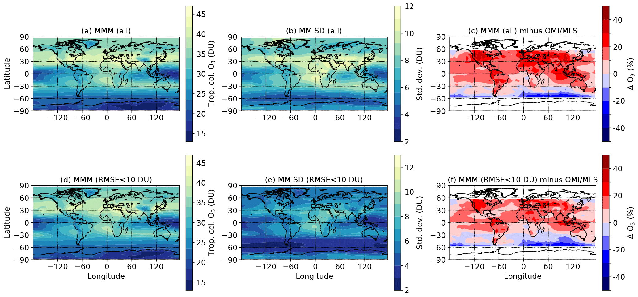
Figure 8Annual-mean year 2005 tropospheric column ozone. (a) The multi-model mean (MMM) of all CCMI models; (b) multi-model standard deviation for the models shown in (a); (c) percent difference between the MMM in (a) and OMI/MLS (MMM minus OMI/MLS); (d) MMM for a subset of CCMI models – those with a root-mean-square error (RMSE) less than 10 DU when compared with OMI (see Fig. 7); (e) multi-model standard deviation for the models shown in (d); (f) percent difference between the MMM in (d) and OMI/MLS (MMM minus OMI/MLS).
Figure 8 shows multi-model means (MMMs) and standard deviations. The MMM in Fig. 8a was calculated for all models, while the MMM in Fig. 8d was calculated only for models with a RMSE less than 10 DU, as indicated in Fig. 7 – i.e. all models except SOCOLv3.0, ACCESS CCM, EMAC-L47, ULAQ-CCM and UMUKCA-UCAM. The CCMI models simulate a global-mean tropospheric ozone abundance of 31.1 DU (Fig. 8a) and 30.2 DU (Fig. 8d), depending on the MMM definition applied. Both global-mean MMMs are close to the OMI/MLS global mean of 28.6 DU (Fig. 2b); however the MMMs differ markedly from OMI/MLS in terms of the global tropospheric ozone distribution.
Compared to OMI/MLS, the models overestimate tropospheric column ozone almost everywhere between 60∘ N and 60∘ S (the region where OMI/MLS data are available), regardless of the MMM definition. The exception is at southern mid-latitudes, where the models underestimate tropospheric ozone compared to OMI/MLS. When the MMM is calculated for all models, the positive bias is up to 50 %, and the negative bias reaches up to −33 % (Fig. 8c). When models with an RMSE >10 DU are discarded from the MMM, the negative bias is largely unchanged at −32 %, but the positive bias is reduced, and reaches up to 40 % (Fig. 8f).
These results broadly agree with models evaluated as part of ACCMIP (Young et al., 2013), and phase 5 of the Coupled Model Intercomparison Project (CMIP5) (Eyring et al., 2013a), which used the same ozone precursor emissions as for CCMI. The ACCMIP models simulated, on average, up to 30 % more tropospheric column ozone compared with OMI/MLS at northern mid-latitudes (Young et al., 2013). The global-annual-mean tropospheric ozone column simulated by these models was 30.8 DU, calculated from 15 models. For the 18 CHEM models participating in CMIP5 (those models with interactive chemistry, i.e. ozone was calculated online and not prescribed from a climatology), the climatological-mean annual-mean MMM averaged over 2000–2005 was 30.5 DU (Eyring et al., 2013a), which is similar to the MMMs calculated here. The CMIP5 and ACCMIP MMMs also show a stronger interhemispheric gradient than OMI/MLS observations do, consistent with our findings.
The standard deviation on the MMM is up to 11.3 DU when calculated for all models (Fig. 8b), and reduces to a maximum of 9.5 DU when calculated for only the models with RMSE <10 DU (Fig. 8e). The variability between models is largest at northern mid-latitudes and in the continental outflow region off the west coast of Africa.
Despite using the ozone precursor emissions recommended for CCMI, SOCOLv3.0 simulates the largest global-mean tropospheric ozone abundance of all the CCMI models (Fig. 6), and exhibits a bias of ∼30 DU regionally compared with OMI/MLS observations (Fig. 2c). The CCMI MMM is biased high in the Northern Hemisphere and low in the Southern Hemisphere compared with OMI/MLS (Fig. 8c and f), consistent with previous studies (ACCMIP and CMIP5). Although ACCMIP, CMIP5 and CCMI all used the same emissions inventories, it is nevertheless interesting that they all produced very similar global-mean tropospheric ozone abundances (approximately 30 DU), given the different foci of the different model intercomparison activities; CCMI focussed on models coupling the stratosphere and troposphere, while CMIP5 focussed on coupling the atmosphere and ocean.
We have developed a new model version, SOCOLv3.1, which includes an upgraded treatment of tropospheric ozone sink processes. This results in a reduction in tropospheric ozone of up to 8 DU (Fig. 2e), which is mostly due to the inclusion of N2O5 hydrolysis on tropospheric aerosol. SOCOLv3.1 still exhibits a positive bias in tropospheric column relative to OMI/MLS (particularly in the Northern Hemisphere), but simulates tropospheric column ozone amounts that are much more comparable with the other CCMI models. Reducing SOCOL's tropospheric ozone bias is expected to lead to improvements in the simulated abundance of species which are oxidized by the hydroxyl radical, such as CO and CH4, since ozone is the primary source of OH. Revell et al. (2015) showed that CO in SOCOLv3 was up to 40 ppbv too low in the Northern Hemisphere compared with observations from TES, due to the tropospheric ozone bias. In SOCOLv3.1, the Northern Hemisphere CO bias is reduced by approximately a factor of 2 (not shown).
We have quantified the contribution to tropospheric ozone variance in SOCOLv3.1 from nine model forcings/parametrizations using GP emulation and sensitivity analysis. By switching off the coupling between chemistry and radiation in the emulator experiments, we aimed to limit dynamical and meteorological variability. We did not consider stratosphere–troposphere exchange in our emulator experiments. Staehelin et al. (2017) showed that SOCOLv3.0's ozone burden due to stratospheric influx, when calculated from ozone origin tracers as described by Garny et al. (2011) and Revell et al. (2015), is close to the multi-model mean values from the ACCMIP and ACCENT ensembles. Therefore, STE is unlikely to be a major driver of SOCOLv3's tropospheric ozone bias. To the best of our knowledge, this is the first time that GP emulation has been applied to global tropospheric ozone modelling. By selecting a relatively small number of model forcings/parametrizations and focussing largely on tropospheric ozone chemistry we aim to demonstrate the utility of the methodology; however it could also be extended to explore the variability in tropospheric ozone due to meteorological parameters.
Our GP emulation experiments and sensitivity analysis illustrate that the ozone precursors NOx, CH4, CO and NMVOCs are responsible for more than 90 % of the variance in tropospheric column ozone in the improved model version, SOCOLv3.1. While CH4 is prescribed as a surface mixing ratio, the other ozone precursors are specified from emissions inventories. Collating emissions inventories is challenging as they are typically compiled using a bottom-up approach. Anthropogenic emissions must rely on accurate reporting, while for biogenic emissions there are no reporting requirements. Furthermore, emissions are generally prescribed in global models as monthly means, and thus do not reflect diurnal or weekly variability (Young et al., 2018). Hassler et al. (2016) identified that current global emissions inventories do not capture trends in the NOx∕CO ratio, and previous multi-model studies have also identified potential deficiencies with the inventories (Parrish et al., 2014; Young et al., 2013). Jena et al. (2015) and Zhong et al. (2016) showed that different NOx emissions inventories can significantly alter simulated tropospheric ozone.
However, it may not be the emissions used for CCMI themselves that are incorrect, but rather problems in how they are handled in global models. Given the coarse grid sizes necessary to run a global model and still retain computational efficiency, resolution – horizontal, vertical and temporal – is likely important for simulating tropospheric ozone, especially in polluted regions where very large emissions in an urban environment may be spread over a model grid cell spanning thousands of square kilometres. In global models, polluted air coming from a point source is considered to be well mixed throughout a large grid cell, which would generally lead to more efficient ozone production (Young et al., 2018). Horizontal and vertical resolution are difficult to test in an emulator sensitivity study as presented here; however by examining the CCMI models collectively (Morgenstern et al., 2017), we can derive some insights. For example, we note that GEOSCCM, HadGEM3-ES and the CESM1 models (CAM4Chem and WACCM), which simulate the smallest RMSEs relative to OMI/MLS (Fig. 7d, e, j, k), have fairly high horizontal resolution relative to other CCMs, of 2∘ × 2∘, 1.875∘ × 1.25∘ and 1.9∘ × 2.5∘, respectively. Of the models analysed in this study, HadGEM3-ES also has the largest number of levels in the troposphere (48). Similarly, tropospheric ozone in the EMAC model with 90 levels (EMAC-L90) compares better with observations than the 47-level version (EMAC-L47) (Fig. 7h, i), which may be due to a more realistic simulation of the ozone gradient across the tropopause (Sect. 3.3).
SOCOLv3.0 uses T42 horizontal resolution (approx. 2.8∘ × 2.8∘), which is also used by CCSRNIES MIROC 3.2 and EMAC. With 16 vertical levels, SOCOLv3.0 has the smallest number of vertical levels in the troposphere out of all the models analysed here, except CCSRNIES MIROC3.2, which has 15. CCSRNIES-MIROC3.2, CNRM-CM5-3 and CMAM do not include any NMVOCs, while SOCOLv3.0 includes only two NMVOCs – isoprene and formaldehyde. Models with complex NMVOC schemes tend to simulate tropospheric ozone favourably compared to OMI/MLS, such as the CESM1 models, with 19 NMVOCs, and GEOSCCM, with 13 explicit NMVOCs.
Another respect in which SOCOLv3.0 is an outlier amongst the CCMI models is its chemical time step of 2 h. The other models analysed in this study have chemical time steps ranging from 6 min (CCSRNIES-MIROC3.2) to 1 h (the models based on the UK Met Office Unified Model, i.e. HadGEM3-ES, NIWA-UKCA, ACCESS and UMUKCA-UCAM). In a sensitivity test, SOCOLv3.0's chemical time step was reduced to 15 min, which reduced the ozone burden in polluted urban areas by approximately 5 DU (not shown). To test how SOCOL responds to prescribing a surface mixing ratio of NOx rather than an emissions flux, we performed a further sensitivity simulation in which surface NO2 mixing ratios from the CESM1 WACCM REF-C1 simulation were prescribed instead of NOx emissions. This also resulted in a reduction of tropospheric ozone of up to 5 DU. In reality there is likely no single solution for reducing SOCOLv3.0's excessive tropospheric ozone bias; however assuming that the prescribed emissions are correct, then increasing the model's spatial and temporal resolution within the bounds of computational efficiency will likely reduce the bias.
We have shown the importance of ozone precursor emissions for simulating the tropospheric ozone budget with SOCOLv3.1. This is in line with the findings of Revell et al. (2015), who analysed three SOCOLv3.0 simulations for the period 1960–2100: REF-C2 (based on RCP 6.0), SEN-C2-fEmis (NOx, CO and NMVOC emissions fixed at constant 1960 levels) and SEN-C2-fEmis-fCH4 (similar to SEN-C2-fEmis but with surface methane concentrations also fixed at constant 1960 levels). They showed that future global ozone abundances are governed largely by changes in methane and NOx, with methane causing an increase in tropospheric ozone that is approximately one-third of that caused by NOx. Future work should investigate how tropospheric ozone evolves in future under the various CCMI sensitivity scenarios in all CCMI models.
Finally, phase 6 of the Coupled Model Intercomparison Project (CMIP6) will use the emissions data set described by Hoesly et al. (2018). In this data set, year 2000 NOx emissions are ∼20 % larger than the emissions used for CCMI (Lamarque et al., 2010). Therefore, simulated ozone biases by the current generation of CCMs will likely be amplified in CMIP6.
Given the results of our multi-model intercomparison as well as previous multi-model studies, our results highlight the need for careful validation of emissions inventories used by global models. However, the way in which emissions are handled by the models also appears to result in biased ozone abundances, and further work is needed to address the challenges of simulating sub-grid processes of importance to tropospheric ozone, in SOCOLv3 as well as in other CCMs. GP emulation may prove a useful tool for such studies, and we have demonstrated its usefulness for understanding tropospheric ozone biases. GP emulation is a powerful tool, and should be considered for use by those wanting to perform detailed sensitivity analyses at low computational cost.
The CCM data used here (except the CESM1 data) are held at the Centre for Environmental Data Analysis (CEDA; http://data.ceda.ac.uk/badc/wcrp-ccmi/data/CCMI-1/, last access: 11 November 2018). CESM1 WACCM and CESM1 CAM4-chem data were downloaded from http://www.earthsystemgrid.org (last access: 11 November 2018). For instructions for access to both archives see http://blogs.reading.ac.uk/ccmi/badc-data-access (IGAC/SPARC Chemistry-Climate Model Initiative, 2018). GEOSCCM data were provided directly by Luke D.Oman to replace the GEOSCCM data currently held in the CEDA archive. SOCOLv3.1 data are available by contacting Laura E. Revell. Matrices for training and testing the GP emulator are in the Supplement.
The supplement related to this article is available online at: https://doi.org/10.5194/acp-18-16155-2018-supplement.
LER and AS designed the experiments and interpreted the output, assisted by FT and AF. All other authors provided information pertaining to their model. LER performed the SOCOL sensitivity simulations and emulator analysis, and wrote the paper with assistance from all other authors.
The authors declare that they have no conflict of interest.
This article is part of the special issue “Chemistry-Climate Modelling Initiative (CCMI) (ACP/AMT/ESSD/GMD inter-journal SI)”. It is not associated with a conference.
We acknowledge the modelling groups for making their simulations available for this analysis, the joint WCRP SPARC–IGAC
Chemistry-Climate Model Initiative (CCMI) for organizing and coordinating the model data analysis activity and the
British Atmospheric Data Centre (BADC) for collecting and archiving the CCMI model output. The EMAC simulations were performed at the
German Climate Computing Centre (DKRZ) through support from the Bundesministerium für Bildung und Forschung (BMBF).
DKRZ and its scientific steering committee are gratefully acknowledged for providing the HPC and data archiving
resources for this consortial project ESCiMo (Earth System Chemistry integrated Modelling). We acknowledge the UK
Met Office for use of the MetUM. This research was partially supported by the New Zealand government's Strategic Science
Investment Fund (SSIF) through the NIWA programme CACV. Olaf Morgenstern acknowledges funding by the New Zealand Royal Society
Marsden Fund (grant 12-NIW-006). The authors wish to acknowledge the contribution of NeSI high-performance computing
facilities to the results of this research. New Zealand's national facilities are provided by the New Zealand eScience
Infrastructure (NeSI) and funded jointly by NeSI's collaborator institutions and through the Ministry of Business,
Innovation and Employment's Research Infrastructure programme (https://www.nesi.org.nz,
last access: 11 November 2018). Fiona Tummon was supported by SNSF
grant number 20F121_138017. ACCESS-CCM runs were supported by the Australian Research Council's Centre of Excellence
for Climate System Science (CE110001028), the Australian government's National Computational Merit Allocation
Scheme (q90) and the Australian Antarctic science grant program (FoRCES 4012). The HadGEM3-ES simulations from the
Met Office were supported by the Joint UK BEIS–Defra Met Office Hadley Centre Climate Programme (GA01101) and
the European Commission's Seventh Framework Programme StratoClim project (grant agreement 603557). CCSRNIES research
was supported by the Environment Research and Technology Development Fund (2-1303 and
2-1709) of the Ministry of the Environment, Japan, and computations were performed on NEC-SX9/A(ECO) computers at
the CGER, NIES. UMUKCA-UCAM model integrations were performed using the ARCHER UK National Supercomputing Service
and MONSooN system, a collaborative facility supplied under the Joint Weather and Climate Research Programme,
which is a strategic partnership between the UK Met Office and the Natural Environment Research Council. Laura E. Revell
thanks China Southern for partial support. The authors thank Edmund Ryan and one anonymous reviewer for their helpful and constructive comments.
Edited by: Paul Young
Reviewed by: Edmund Ryan and one anonymous referee
Arfeuille, F., Luo, B. P., Heckendorn, P., Weisenstein, D., Sheng, J. X., Rozanov, E., Schraner, M., Brönnimann, S., Thomason, L. W., and Peter, T.: Modeling the stratospheric warming following the Mt. Pinatubo eruption: uncertainties in aerosol extinctions, Atmos. Chem. Phys., 13, 11221–11234, https://doi.org/10.5194/acp-13-11221-2013, 2013. a
Auvray, M. and Bey, I.: Long-range transport to Europe: Seasonal variations and implications for the European ozone budget, J. Geophys. Res.-Atmos., 110, D11303, https://doi.org/10.1029/2004JD005503, 2005. a
Carslaw, K. S., Lee, L. A., Reddington, C. L., Pringle, K. J., Rap, A., Forster, P. M., Mann, G. W., Spracklen, D. V., Woodhouse, M. T., Regayre, L. A., and Pierce, J. R.: Large contribution of natural aerosols to uncertainty in indirect forcing, Nature, 503, 67–71, https://doi.org/10.1038/nature12674, 2013. a
Chang, J. S., Brost, R. A., Isaksen, I. S. A., Madronich, S., Middleton, P., Stockwell, W. R., and Walcek, C. J.: A three-dimensional Eulerian acid deposition model: Physical concepts and formulation, J. Geophys. Res.-Atmos., 92, 14681–14700, https://doi.org/10.1029/JD092iD12p14681, 1987. a
Denman, K. L., Brasseur, G., Chidthaisong, A., Ciais, P., Cox, P. M., Dickinson, R. E., Hauglustaine, D., Heinze, C., Holland, E., Jacob, D., Lohmann, U., Ramachandran, S., da Silva Dias, P. L., Wofsy, S. C., and Zhang, X.: Couplings between changes in the climate system and biogeochemistry, Chapter 7 in Climate Change 2007: the Physical Science Basis. Contribution of Working Group I to the Fourth Assessment Report of the Intergovernmental Panel on Climate Change, edited by: Solomon, S., Qin, D., Manning, M., Chen, Z., Marquis, M., Averyt, K. B., Tignor, M., and Miller, H. L., Cambridge University Press, Cambridge, United Kingdom and New York, NY, USA, 2007. a
Dietmüller, S., Eichinger, R., Garny, H., Birner, T., Boenisch, H., Pitari, G., Mancini, E., Visioni, D., Stenke, A., Revell, L., Rozanov, E., Plummer, D. A., Scinocca, J., Jöckel, P., Oman, L., Deushi, M., Kiyotaka, S., Kinnison, D. E., Garcia, R., Morgenstern, O., Zeng, G., Stone, K. A., and Schofield, R.: Quantifying the effect of mixing on the mean age of air in CCMVal-2 and CCMI-1 models, Atmos. Chem. Phys., 18, 6699–6720, https://doi.org/10.5194/acp-18-6699-2018, 2018. a
Egorova, T. A., Rozanov, E. V., Zubov, V. A., and Karol, I. L.: Model for investigating ozone trends (MEZON), Izv. Atmos. Ocean. Phy., 39, 277–292, 2003. a
Ehhalt, D., Prather, M., Dentener, F., Derwent, R., Dlugokencky, E., Holland, E., Isaksen, I., Katima, J., Kirchhoff, V., Matson, P., Midgley, P., and Wang, M.: Atmospheric chemistry and greenhouse gases, Chapter 4 in Climate Change 2001: The Scientific Basis. Contribution ofWorking Group I to the Third Assessment Report of the Intergovernmental Panel on Climate Change, edited by: Houghton, J. T., Ding, Y., Griggs, D. J., Noguer, M., van der Linden, P. J., Dai, X., Maskell, K., and Johnson, C. A., Cambridge University Press, Cambridge, United Kingdom and New York, NY, USA, 2001. a
ETH-PMOD: Swiss Federal Institute of Technology Zurich and the Physical-Meteorology Observatory Davos, Data, Part of the Chemistry-Climate Model Initiative (CCMI-1) Project Database, NCAS British Atmospheric Data Centre, available at: http://catalogue.ceda.ac.uk/uuid/1005d2c25d14483aa66a5f4a7f50fcf0 (last access: 28 September 2017), 2015. a
Evans, M. J. and Jacob, D. J.: Impact of new laboratory studies of N2O5 hydrolysis on global model budgets of tropospheric nitrogen oxides, ozone and OH, Geophys. Res. Lett., 32, L09813, https://doi.org/10.1029/2005GL022469, 2005. a
Eyring, V., Arblaster, J. M., Cionni, I., Sedláček, J., Perlwitz, J., Young, P. J., Bekki, S., Bergmann, D., Cameron-Smith, P., Collins, W. J., Faluvegi, G., Gottschaldt, K. D., Horowitz, L. W., Kinnison, D. E., Lamarque, J. F., Marsh, D. R., Saint-Martin, D., Shindell, D.T., Sudo, K., Szopa, S., and Watanabe, S.: Long-term ozone changes and associated climate impacts in CMIP5 simulations, J. Geophys. Res., 118, 5029–5060, https://doi.org/10.1002/jgrd.50316, 2013a. a, b
Eyring, V., Lamarque, J.-F., Hess, P., Arfeuille, F., Bowman, K., Chipperfield, M. P., Duncan, B., Fiore, A., Gettelman, A., Giorgetta, M. A., Granier, C., Hegglin, M., Kinnison, D., Kunze, M., Langematz, U., Luo, B., Martin, R., Matthes, K., Newman, P. A., Peter, T., Robock, A., Ryerson, T., Saiz-Lopez, A., Salawitch, R., Schultz, M., Shepherd, T. G., Shindell, D., Staehelin, J., Tegtmeier, S., Thomason, L., Tilmes, S., Vernier, J.-P., Waugh, D. W., and Young, P. J.: Overview of IGAC/SPARC Chemistry-Climate Model Initiative (CCMI) Community Simulations in Support of Upcoming Ozone and Climate Assessments, SPARC Newsletter no. 40, ISSN 1245-4680, 48–66, 2013b. a, b
Garny, H., Grewe, V., Dameris, M., Bodeker, G. E., and Stenke, A.: Attribution of ozone changes to dynamical and chemical processes in CCMs and CTMs, Geosci. Model Dev., 4, 271–286, https://doi.org/10.5194/gmd-4-271-2011, 2011. a
Gaudel, A., Cooper, O. R., Ancellet G., Barret, B., Boynard, A., Burrows, J. P., et al.: Tropospheric Ozone Assessment Report: Present-day distribution and trends of tropospheric ozone relevant to climate and global atmospheric chemistry model evaluation, Elem. Sci. Anth., 6, 59, https://doi.org/10.1525/elementa.291, 2018. a
Greenslade, J. W., Alexander, S. P., Schofield, R., Fisher, J. A., and Klekociuk, A. K.: Stratospheric ozone intrusion events and their impacts on tropospheric ozone in the Southern Hemisphere, Atmos. Chem. Phys., 17, 10269–10290, https://doi.org/10.5194/acp-17-10269-2017, 2017. a
Guenther, A., Karl, T., Harley, P., Wiedinmyer, C., Palmer, P. I., and Geron, C.: Estimates of global terrestrial isoprene emissions using MEGAN (Model of Emissions of Gases and Aerosols from Nature), Atmos. Chem. Phys., 6, 3181–3210, https://doi.org/10.5194/acp-6-3181-2006, 2006. a
Hassler, B., McDonald, B. C., Frost, G. J., Borbon, A., Carslaw, D. C., Civerolo, K., Granier, C., Monks, P. S., Monks, S., Parrish, D. D., Pollack, I. B., Rosenlof, K. H., Ryerson, T. B., von Schneidemesser, E., and Trainer, M.: Analysis of long-term observations of NOx and CO in megacities and application to constraining emissions inventories, Geophys. Res. Lett., 43, 9920–9930, https://doi.org/10.1002/2016GL069894, 2016. a
Hauglustaine, D. A., Granier, C., Brasseur, G., and Megie G.: The importance of atmospheric chemistry in the calculation of radiative forcing on the climate system, J. Geophys. Res., 99, 1173–1186, 1994. a
Hoesly, R. M., Smith, S. J., Feng, L., Klimont, Z., Janssens-Maenhout, G., Pitkanen, T., Seibert, J. J., Vu, L., Andres, R. J., Bolt, R. M., Bond, T. C., Dawidowski, L., Kholod, N., Kurokawa, J.-I., Li, M., Liu, L., Lu, Z., Moura, M. C. P., O'Rourke, P. R., and Zhang, Q.: Historical (1750–2014) anthropogenic emissions of reactive gases and aerosols from the Community Emissions Data System (CEDS), Geosci. Model Dev., 11, 369–408, https://doi.org/10.5194/gmd-11-369-2018, 2018. a
IGAC/SPARC Chemistry-Climate Model Initiative: BADC data access, available at: http://blogs.reading.ac.uk/ccmi/badc-data-access, last access: 11 November 2018.
Jena, C., Ghude, S. D., Beig, G., Chate, D. M., Kumar, R., Pfister, G. G., Lal, D. M., Surendran, D. E., Fadnavis, S., and van der A, R. J.: Inter-comparison of different NOx inventories and associated variation in simulated surface ozone in Indian region, Atmos. Environ., 117, 61–73, https://doi.org/10.1016/j.atmosenv.2015.06.057, 2015. a
Jöckel, P., Tost, H., Pozzer, A., Kunze, M., Kirner, O., Brenninkmeijer, C. A. M., Brinkop, S., Cai, D. S., Dyroff, C., Eckstein, J., Frank, F., Garny, H., Gottschaldt, K.-D., Graf, P., Grewe, V., Kerkweg, A., Kern, B., Matthes, S., Mertens, M., Meul, S., Neumaier, M., Nützel, M., Oberländer-Hayn, S., Ruhnke, R., Runde, T., Sander, R., Scharffe, D., and Zahn, A.: Earth System Chemistry integrated Modelling (ESCiMo) with the Modular Earth Submodel System (MESSy) version 2.51, Geosci. Model Dev., 9, 1153–1200, https://doi.org/10.5194/gmd-9-1153-2016, 2016. a
Johnson, J. S., Cui, Z., Lee, L. A., Gosling, J. P., Blyth, A. M., and Carslaw, K. S.: Evaluating uncertainty in convective cloud microphysics using statistical emulation, J. Adv. Model. Earth Syst., 7, 162–187, https://doi.org/10.1002/2014MS000383, 2015. a
Kerkweg, A., Buchholz, J., Ganzeveld, L., Pozzer, A., Tost, H., and Jöckel, P.: Technical Note: An implementation of the dry removal processes DRY DEPosition and SEDImentation in the Modular Earth Submodel System (MESSy), Atmos. Chem. Phys., 6, 4617–4632, https://doi.org/10.5194/acp-6-4617-2006, 2006. a
Köpke, P., Hess, M., Schult, I., and Shettle, E. P.: Global Aerosol Data Set, Max-Planck-Institut für Meteorologie, Hamburg, Report No. 243, available at: https://www.mpimet.mpg.de/fileadmin/publikationen/Reports/MPI-Report_243.pdf (last access: 25 September 2017), 1997. a
Lamarque, J.-F., Bond, T. C., Eyring, V., Granier, C., Heil, A., Klimont, Z., Lee, D., Liousse, C., Mieville, A., Owen, B., Schultz, M. G., Shindell, D., Smith, S. J., Stehfest, E., Van Aardenne, J., Cooper, O. R., Kainuma, M., Mahowald, N., McConnell, J. R., Naik, V., Riahi, K., and van Vuuren, D. P.: Historical (1850–2000) gridded anthropogenic and biomass burning emissions of reactive gases and aerosols: methodology and application, Atmos. Chem. Phys., 10, 7017–7039, https://doi.org/10.5194/acp-10-7017-2010, 2010. a, b
Lee, L. A., Carslaw, K. S., Pringle, K. J., Mann, G. W., and Spracklen, D. V.: Emulation of a complex global aerosol model to quantify sensitivity to uncertain parameters, Atmos. Chem. Phys., 11, 12253–12273, https://doi.org/10.5194/acp-11-12253-2011, 2011. a
Lee, L. A., Carslaw, K. S., Pringle, K. J., and Mann, G. W.: Mapping the uncertainty in global CCN using emulation, Atmos. Chem. Phys., 12, 9739–9751, https://doi.org/10.5194/acp-12-9739-2012, 2012. a
Le Gratiet, L., Marelli, S., and Sudret, B.: Metamodel-Based Sensitivity Analysis: Polynomial Chaos Expansions and Gaussian Processes, in: Handbook of Uncertainty Quantification, edited by: Ghanem, R., Higdon, D., and Owhadi, H., Springer, https://doi.org/10.1007/978-3-319-12385-1_38, 2017. a
Lin, M., Horowitz, L. W., Oltmans, S. J., Fiore, A. M., and Fan, S.: Tropospheric ozone trends at Mauna Loa Observatory tied to decadal climate variability, Nat. Geosci., 7, 136–143, https://doi.org/10.1038/ngeo2066, 2014. a
Loeppky, J. L., Sacks, J., and Welch, W. J.: Choosing the sample size of a computer experiment: A Practical Guide, Technometrics, 51, 366–376, https://doi.org/10.1198/TECH.2009.08040, 2009. a
Luhar, A. K., Galbally, I. E., Woodhouse, M. T., and Thatcher, M.: An improved parameterisation of ozone dry deposition to the ocean and its impact in a global climate-chemistry model, Atmos. Chem. Phys., 17, 3749–3767, https://doi.org/10.5194/acp-17-3749-2017, 2017. a
Luo, B.: Stratospheric aerosol data for use in CCMI models, available at: ftp://iacftp.ethz.ch/pub_read/luo/ccmi/ (last access: 29 August 2018), 2013. a
Masui, T., Matsumoto, K., Hijioka, Y., Kinoshita, T., Nozawa, T., Ishiwatari, S., Kato, E., Shukla, P. R., Yamagata, Y., and Kainuma, M.: An emission pathway for stabilization at 6 Wm-2 radiative forcing, Climatic Change, 109, 59, https://doi.org/10.1007/s10584-011-0150-5, 2011. a
McKay, M., Conover, W., and Beckman, R.: A comparison of three methods for selecting values of input variables in the analysis of output from a computer code, Technometrics, 21, 239–245, https://doi.org/10.2307/1268522, 1979. a
Morgenstern, O., Hegglin, M. I., Rozanov, E., O'Connor, F. M., Abraham, N. L., Akiyoshi, H., Archibald, A. T., Bekki, S., Butchart, N., Chipperfield, M. P., Deushi, M., Dhomse, S. S., Garcia, R. R., Hardiman, S. C., Horowitz, L. W., Jöckel, P., Josse, B., Kinnison, D., Lin, M., Mancini, E., Manyin, M. E., Marchand, M., Marécal, V., Michou, M., Oman, L. D., Pitari, G., Plummer, D. A., Revell, L. E., Saint-Martin, D., Schofield, R., Stenke, A., Stone, K., Sudo, K., Tanaka, T. Y., Tilmes, S., Yamashita, Y., Yoshida, K., and Zeng, G.: Review of the global models used within phase 1 of the Chemistry-Climate Model Initiative (CCMI), Geosci. Model Dev., 10, 639–671, https://doi.org/10.5194/gmd-10-639-2017, 2017. a, b, c, d, e
Myhre, G., Shindell, D., Bréon, F.-M., Collins, W., Fuglestvedt, J., Huang, J., Koch, D., Lamarque, J.-F., Lee, D., Mendoza, B., Nakajima, T., Robock, A., Stephens, G., Takemura, T., and Zhang, H.: Anthropogenic and natural radiative forcing, Chapter 8 in Climate Change 2013: The Physical Science Basis. Contribution of Working Group I to the Fifth Assessment Report of the Intergovernmental Panel on Climate Change, edited by: Stocker, T. F., Qin, D., Plattner, G.-K., Tignor, M., Allen, S. K., Boschung, J., Nauels, A., Xia, Y., Bex, V., and Midgley, P. M., Cambridge University Press, Cambridge, United Kingdom and New York, NY, USA, 2013. a
Nicely, J. M., Hanisco, T. F., Deushi, M., Duncan, B. N., Haslerud, A. S., Jöckel, P., Josse, B., Kinnison, D. E., Klekociuk, A., Manyin, M. E., Morgenstern, O., Murray, L. T., Myhre, G., Oman, L. D., Pitari, G., Pozzer, A., Revell, L. E., Rozanov, E., Salawitch, R. J., Stenke, A., Stone, K., Strahan, S., Tilmes, S., Tost, H., Westervelt, D. M., and Zeng, G.: Hydroxyl radical intercomparison between chemistry-climate model and chemical transport model simulations for CCMI-1, in preparation, 2018. a
O'Hagan, A.: Bayesian analysis of computer code outputs: A tutorial, Reliab. Eng. Syst. Safe., 91, 1290–1300, https://doi.org/10.1016/j.ress.2005.11.025, 2006. a, b
Orbe, C., Yang, H., Waugh, D. W., Zeng, G., Morgenstern , O., Kinnison, D. E., Lamarque, J.-F., Tilmes, S., Plummer, D. A., Scinocca, J. F., Josse, B., Marecal, V., Jöckel, P., Oman, L. D., Strahan, S. E., Deushi, M., Tanaka, T. Y., Yoshida, K., Akiyoshi, H., Yamashita, Y., Stenke, A., Revell, L., Sukhodolov, T., Rozanov, E., Pitari, G., Visioni, D., Stone, K. A., Schofield, R., and Banerjee, A.: Large-scale tropospheric transport in the Chemistry-Climate Model Initiative (CCMI) simulations, Atmos. Chem. Phys., 18, 7217–7235, https://doi.org/10.5194/acp-18-7217-2018, 2018. a
Parrish, D. D., Lamarque, J. F., Naik, V., Horowitz, L., Shindell, D. T., Staehelin, J., Derwent, R., Cooper, O. R., Tanimoto, H., Volz-Thomas, A., Gilge, S., Scheel, H. E., Steinbacher, M., and Fröhlich, M.: Long-term changes in lower tropospheric baseline ozone concentrations: Comparing chemistry-climate models and observations at northern midlatitudes, J. Geophys. Res.-Atmos., 119, 5719–5736, https://doi.org/10.1002/2013JD021435, 2014. a, b
Pöschl, U., von Kuhlmann, R., Poisson, N., and Crutzen, P. J.: Development and Intercomparison of Condensed Isoprene Oxidation Mechanisms for Global Atmospheric Modeling, J. Atmos. Chem., 37, 29–52, https://doi.org/10.1023/a:1006391009798, 2000. a
Rayner, N. A., Parker, D. E., Horton, E. B., Folland, C. K., Alexander, L. V., Rowell, D. P., Kent, E. C., and Kaplan, A.: Global analyses of sea surface temperature, sea ice, and night marine air temperature since the late nineteenth century, J. Geophys. Res.-Atmos., 108, 4407, https://doi.org/10.1029/2002JD002670, 2003. a
Revell, L. E., Tummon, F., Stenke, A., Sukhodolov, T., Coulon, A., Rozanov, E., Garny, H., Grewe, V., and Peter, T.: Drivers of the tropospheric ozone budget throughout the 21st century under the medium-high climate scenario RCP 6.0, Atmos. Chem. Phys., 15, 5887–5902, https://doi.org/10.5194/acp-15-5887-2015, 2015. a, b, c, d, e, f, g, h, i
Riahi, K., Rao, S., Krey, V., Cho, C., Chirkov, V., Fischer, G., Kindermann, G., Nakicenovic, N., and Rafaj, P.: RCP 8.5 – A scenario of comparatively high greenhouse gas emissions, Climatic Change, 109, 33, https://doi.org/10.1007/s10584-011-0149-y, 2011. a
Roeckner, E., Bäuml, G., Bonaventura, L., Brokopf, R., Esch, M., Giorgetta, M., Hagemann, S., Kirchner, I., Kornblueh, L., Manzini, E., Rhodin, A., Schlese, U., Schulzweida, U., and Tompkins, A.: The atmospheric general circulation model ECHAM 5. Part I: Model description, Max-Planck-Institut für Meteorologie, Hamburg, Report No. 349, available at: http://www.mpimet.mpg.de/fileadmin/publikationen/Reports/max_scirep_349.pdf (last access: 28 September 2017), 2003. a
Rozanov, E., Schlesinger, M. E., Zubov, V., Yang, F., and Andronova, N. G.: The UIUC three-dimensional stratospheric chemical transport model: Description and evaluation of the simulated source gases and ozone, J. Geophys. Res., 104, 11755–11781, 1999. a
Ryan, E., Wild, O., Voulgarakis, A., and Lee, L.: Fast sensitivity analysis methods for computationally expensive models with multi-dimensional output, Geosci. Model Dev., 11, 3131–3146, https://doi.org/10.5194/gmd-11-3131-2018, 2018. a
Sillman, S., Logan, J. A., and Wofsy, S. C.: The sensitivity of ozone to nitrogen oxides and hydrocarbons in regional ozone episodes, J. Geophys. Res.-Atmos., 95, 1837–1851, https://doi.org/10.1029/JD095iD02p01837, 1990. a
Silva, R. A., West, J. J., Zhang, Y., Anenberg, S. C., Lamarque, J.-F., Shindell, D. T., Collins, W. J., Dalsoren, S., Faluvegi, G., Folberth, G., Horowitz, L. W., Nagashima, T., Naik, V., Rumbold, S., Skeie, R., Sudo, K., Takemura, T., Bergmann, D., Cameron-Smith, P., Cionni, I., Doherty, R. M., Eyring, V., Josse, B., MacKenzie, I. A., Plummer, D., Righi, M., Stevenson, D. S., Strode, S., Szopa, S., and Zeng, G.: Global premature mortality due to anthropogenic outdoor air pollution and the contribution of past climate change, Environ. Res. Lett., 8, 034005, https://doi.org/10.1088/1748-9326/8/3/034005, 2013. a
Silva, R. A., West, J. J., Lamarque, J.-F., Shindell, D. T., Collins, W. J., Faluvegi, G., Folberth, G. A., Horowitz, L. W., Nagashima, T., Naik, V., Rumbold, S. T., Sudo, K., Takemura, T., Bergmann, D., Cameron-Smith, P., Doherty, R. M., Josse, B., MacKenzie, I. A., Stevenson, D. S., and Zeng, G.: Future global mortality from changes in air pollution attributable to climate change, Nat. Clim. Change, 7, 647–651, https://doi.org/10.1038/nclimate3354, 2017. a
SPARC CCMVal: SPARC Report on the Evaluation of Chemistry-Climate Models, edited by: Eyring, V., Shepherd, T. G., and Waugh, D. W., SPARC Report No. 5, WCRP-132, WMO/TD-No. 1526, available at: http://www.sparc-climate.org/publications/sparc-reports/sparc-report-no-5/ (last access: 31 May 2018), 2010. a
Staehelin, J., Tummon, F., Revell, L. E., Stenke, A., and Peter, T.: Tropospheric ozone at northern mid-latitudes: modeled and measured long-term changes, Atmosphere, 8, 163, 9, https://doi.org/10.3390/atmos8090163, 2017. a, b, c, d
Stenke, A., Schraner, M., Rozanov, E., Egorova, T., Luo, B., and Peter, T.: The SOCOL version 3.0 chemistry-climate model: description, evaluation, and implications from an advanced transport algorithm, Geosci. Model Dev., 6, 1407–1427, https://doi.org/10.5194/gmd-6-1407-2013, 2013. a
Stevenson, D. S., Dentener, F. J., Schultz, M. G., Ellingsen, K., van Noije, T. P. C., Wild, O., Zeng, G., Amann, M., Atherton, C. S., Bell, N., Bergmann, D. J., Bey, I., Butler, T., Cofala, J., Collins, W. J., Derwent, R. G., Doherty, R. M., Drevet, J., Eskes, H. J., Fiore, A. M., Gauss, M., Hauglustaine, D. A., Horowitz, L. W., Isaksen, I. S. A., Krol, M.C., Lamarque, J.-F., Lawrence, M. G., Montanaro, V., Müller, J.-F., Pitari, G., Prather, M. J., Pyle, J. A., Rast, S., Rodriguez, J. M., Sanderson, M. G., Savage, N. H., Shindell, D. T., Strahan, S. E., Sudo, K., and Szopa, S.: Multimodel ensemble simulations of present-day and near-future tropospheric ozone, J. Geophys. Res.-Atmos., 111, D08301, https://doi.org/10.1029/2005JD006338, 2006. a
Stevenson, D. S., Young, P. J., Naik, V., Lamarque, J.-F., Shindell, D. T., Voulgarakis, A., Skeie, R. B., Dalsoren, S. B., Myhre, G., Berntsen, T. K., Folberth, G. A., Rumbold, S. T., Collins, W. J., MacKenzie, I. A., Doherty, R. M., Zeng, G., van Noije, T. P. C., Strunk, A., Bergmann, D., Cameron-Smith, P., Plummer, D. A., Strode, S. A., Horowitz, L., Lee, Y. H., Szopa, S., Sudo, K., Nagashima, T., Josse, B., Cionni, I., Righi, M., Eyring, V., Conley, A., Bowman, K. W., Wild, O., and Archibald, A.: Tropospheric ozone changes, radiative forcing and attribution to emissions in the Atmospheric Chemistry and Climate Model Intercomparison Project (ACCMIP), Atmos. Chem. Phys., 13, 3063–3085, https://doi.org/10.5194/acp-13-3063-2013, 2013. a
Thornton, J. A., Wooldridge, P. J., Cohen, R. C., Martinez, M., Harder, H., Brune, W. H., Williams, E. J., Roberts, J. M., Fehsenfeld, F. C., Hall, S. R., Shetter, R. E., Wert, B. P., and Fried, A.: Ozone production rates as a function of NOx abundances and HOx production rates in the Nashville urban plume, J. Geophys. Res.-Atmos., 107, ACH 7-1–ACH 7-17, https://doi.org/10.1029/2001JD000932, 2002. a
Wesely, M.: Parameterization of the surface resistances to gaseous dry deposition in regional-scale numerical models, Atmos. Environ., 23, 1293–1304, 1989. a, b
World Meteorological Organization: Scientific Assessment of Ozone Depletion: 2010, WMO Global Ozone Research and Monitoring Project – Report No. 52, Geneva, Switzerland, 2011. a
Young, P. J., Archibald, A. T., Bowman, K. W., Lamarque, J.-F., Naik, V., Stevenson, D. S., Tilmes, S., Voulgarakis, A., Wild, O., Bergmann, D., Cameron-Smith, P., Cionni, I., Collins, W. J., Dalsøren, S. B., Doherty, R. M., Eyring, V., Faluvegi, G., Horowitz, L. W., Josse, B., Lee, Y. H., MacKenzie, I. A., Nagashima, T., Plummer, D. A., Righi, M., Rumbold, S. T., Skeie, R. B., Shindell, D. T., Strode, S. A., Sudo, K., Szopa, S., and Zeng, G.: Pre-industrial to end 21st century projections of tropospheric ozone from the Atmospheric Chemistry and Climate Model Intercomparison Project (ACCMIP), Atmos. Chem. Phys., 13, 2063–2090, https://doi.org/10.5194/acp-13-2063-2013, 2013. a, b, c, d, e
Young, P. J., Naik, V., Fiore, A. M., Gaudel, A., Guo, J., Lin, M. Y., Neu, J. L., Parrish, D. D., Rieder, H. E., Schnell, J. L., Tilmes, S., Wild, O., Zhang, L., Ziemke, J., Brandt, J., Delcloo, A., Doherty, R. M., Geels, C., Hegglin, M. I., Hu, L., Im, U., Kumar, R., Luhar, A., Murray, L., Plummer, D., Rodriguez, J., Saiz-Lopez, A., Schultz, M. G., Woodhouse, M. T., and Zeng, G.: Tropospheric Ozone Assessment Report: Assessment of global-scale model performance for global and regional ozone distributions, variability, and trends, Elem. Sci. Anth., 6, 1, https://doi.org/10.1525/elementa.265, 2018. a, b, c
Zhong, M., Saikawa, E., Liu, Y., Naik, V., Horowitz, L. W., Takigawa, M., Zhao, Y., Lin, N.-H., and Stone, E. A.: Air quality modeling with WRF-Chem v3.5 in East Asia: sensitivity to emissions and evaluation of simulated air quality, Geosci. Model Dev., 9, 1201–1218, https://doi.org/10.5194/gmd-9-1201-2016, 2016. a
Ziemke, J. R., Chandra, S., Duncan, B. N., Froidevaux, L., Bhartia, P. K., Levelt, P. F., and Waters, J. W.: Tropospheric ozone determined from Aura OMI and MLS: Evaluation of measurements and comparison with the Global Modeling Initiative's Chemical Transport Model, J. Geophys. Res.-Atmos., 111, D19303, https://doi.org/10.1029/2006JD007089, 2006. a