Monitoring global tropospheric OH concentrations using satellite observations of atmospheric methane

Zhang, Yuzhong; Jacob, Daniel J.; Maasakkers, Joannes D.; Sulprizio, Melissa P.; Sheng, Jian-Xiong; Gautam, Ritesh; Worden, John

doi:https://doi.org/10.5194/acp-18-15959-2018

Articles | Volume 18, issue 21

https://doi.org/10.5194/acp-18-15959-2018

Articles | Volume 18, issue 21

Research article

07 Nov 2018

Research article |

| 07 Nov 2018

Monitoring global tropospheric OH concentrations using satellite observations of atmospheric methane

Yuzhong Zhang, Daniel J. Jacob, Joannes D. Maasakkers, Melissa P. Sulprizio, Jian-Xiong Sheng, Ritesh Gautam, and John Worden

Abstract

The hydroxyl radical (OH) is the main tropospheric oxidant and the main sink for atmospheric methane. The global abundance of OH has been monitored for the past decades using atmospheric methyl chloroform (CH₃CCl₃) as a proxy. This method is becoming ineffective as atmospheric CH₃CCl₃ concentrations decline. Here we propose that satellite observations of atmospheric methane in the short-wave infrared (SWIR) and thermal infrared (TIR) can provide an alternative method for monitoring global OH concentrations. The premise is that the atmospheric signature of the methane sink from oxidation by OH is distinct from that of methane emissions. We evaluate this method in an observing system simulation experiment (OSSE) framework using synthetic SWIR and TIR satellite observations representative of the TROPOMI and CrIS instruments, respectively. The synthetic observations are interpreted with a Bayesian inverse analysis, optimizing both gridded methane emissions and global OH concentrations. The optimization is done analytically to provide complete error accounting, including error correlations between posterior emissions and OH concentrations. The potential bias caused by prior errors in the 3-D seasonal OH distribution is examined using OH fields from 12 different models in the ACCMIP archive. We find that the satellite observations of methane have the potential to constrain the global tropospheric OH concentration with a precision better than 1 % and an accuracy of about 3 % for SWIR and 7 % for TIR. The inversion can successfully separate the effects of perturbations to methane emissions and to OH concentrations. Interhemispheric differences in OH concentrations can also be successfully retrieved. Error estimates may be overoptimistic because we assume in this OSSE that errors are strictly random and have no systematic component. The availability of TROPOMI and CrIS data will soon provide an opportunity to test the method with actual observations.

How to cite

How to cite.

Dates

Received: 09 May 2018 – Discussion started: 29 May 2018 – Revised: 04 Sep 2018 – Accepted: 26 Sep 2018 – Published: 07 Nov 2018

1 Introduction

The hydroxyl radical (OH) is the main oxidant in the troposphere, responsible for the oxidation of a wide range of gases including nitrogen oxides ( ${NO}_{x} \equiv NO + {NO}_{2}$ ), sulfur dioxide (SO₂), carbon monoxide (CO), methane, and other volatile organic compounds (VOCs). Subsequent reactions can lead to the formation of tropospheric ozone, strong acids, and organic aerosol. Monitoring of global tropospheric OH concentrations and its trends is a central problem in atmospheric chemistry. Here we show that satellite observations of atmospheric methane can provide a powerful vehicle for this purpose.

The chemistry controlling tropospheric OH concentrations is complex (Levy, 1971; Logan et al., 1981). The primary source is photolysis of ozone in the presence of water vapor. OH then reacts with CO and VOCs on a timescale of ∼1 s to produce peroxy radicals, which can be converted back to OH by reaction with NO. This cycling of radicals is terminated by conversion to non-radical forms, principally peroxides. The dependences of OH concentrations on natural and anthropogenic emissions of NO_x, CO, and VOCs, as well as on UV radiation and humidity, are complicated and poorly established (Holmes et al., 2013; Murray et al., 2013; Monks et al., 2015).

OH concentrations are highly variable spatially and temporally, making it nearly impossible to infer global mean OH concentration from sparse direct measurements, which are difficult by themselves because of the low concentrations (∼10⁶ molecules cm⁻³). Singh (1977) and Lovelock (1977) first pointed out the possibility of estimating the global mean OH concentration through atmospheric measurements of methyl chloroform (CH₃CCl₃), an industrial solvent. The industrial production of methyl chloroform is well known, and essentially all of this production is eventually released to the atmosphere, where it mixes globally in the troposphere and is removed by oxidation by OH. From measurements of atmospheric methyl chloroform and knowledge of the source, one deduces by mass balance a methyl chloroform lifetime against oxidation by tropospheric OH of 6.3±0.4 years (Prather et al., 2012), providing a proxy for the global mean tropospheric OH concentration. The method became more accurate after the global ban on methyl chloroform production under the Montreal Protocol in the 1990s, as the source could then be assumed to be close to zero (Montzka et al., 2011). Estimates of annual and decadal OH variability can be obtained from the long-term methyl chloroform record (Prinn et al., 2001; Krol and Lelieveld, 2003; Bousquet et al., 2005; Montzka et al., 2011). Compared to estimates from the methyl chloroform proxy, global tropospheric chemistry models tend to predict higher OH concentrations (Voulgarakis et al., 2013; Naik et al., 2013), smaller interannual variability (Holmes et al., 2013; Murray et al., 2013), and larger long-term trends (Holmes et al., 2013).

Understanding the factors controlling OH concentrations and its trends is particularly important for interpretation of methane trends. Methane is the second most important anthropogenic greenhouse gas after CO₂ and has contributed to about a quarter of the climate warming from pre-industrial times to present (Myhre et al., 2013). About 90 % of atmospheric methane is lost through oxidation by tropospheric OH (Kirschke et al., 2013). Atmospheric methane rose by 1 %–2 % a⁻¹ in the 1970s and 1980s, stopped growing in the late 1990s, and has resumed a steady growth of 0.3 %–0.7 % a⁻¹ since 2006 (Rigby et al., 2008; Dlugokencky et al., 2009; Hartmann et al., 2013). Interpretation of these trends has generally focused on changing emissions (Rice et al., 2016; Hausmann et al., 2016; Nisbet et al., 2016; Schaefer et al., 2016), but recent studies have suggested that the growth over the past decade could be contributed by a decline in global OH concentration (Turner et al., 2017; Rigby et al., 2017). On the other hand, the trend in atmospheric CO over the past decade suggests an increase in global OH concentrations (Gaubert et al., 2017).

Inferring OH trends from methyl chloroform will become more difficult in the future as concentrations approach the detection limit (Liang et al., 2017), and possible evasion from the ocean may complicate interpretation (Wennberg et al., 2004). Finding an alternative proxy for tropospheric OH is viewed as a pressing problem in the atmospheric chemistry community (Lelieveld et al., 2006). Huang and Prinn (2002) pointed out that the major limitation to hydrochlorofluorocarbons and hydrofluorocarbons as alternative proxies is the lack of accurate estimates of global emissions. Liang et al. (2017) proposed to use the interhemispheric gradients of a suite of these compounds to jointly retrieve global emissions and tropospheric OH, but their approach may be limited by the sparsity of the surface observation network.

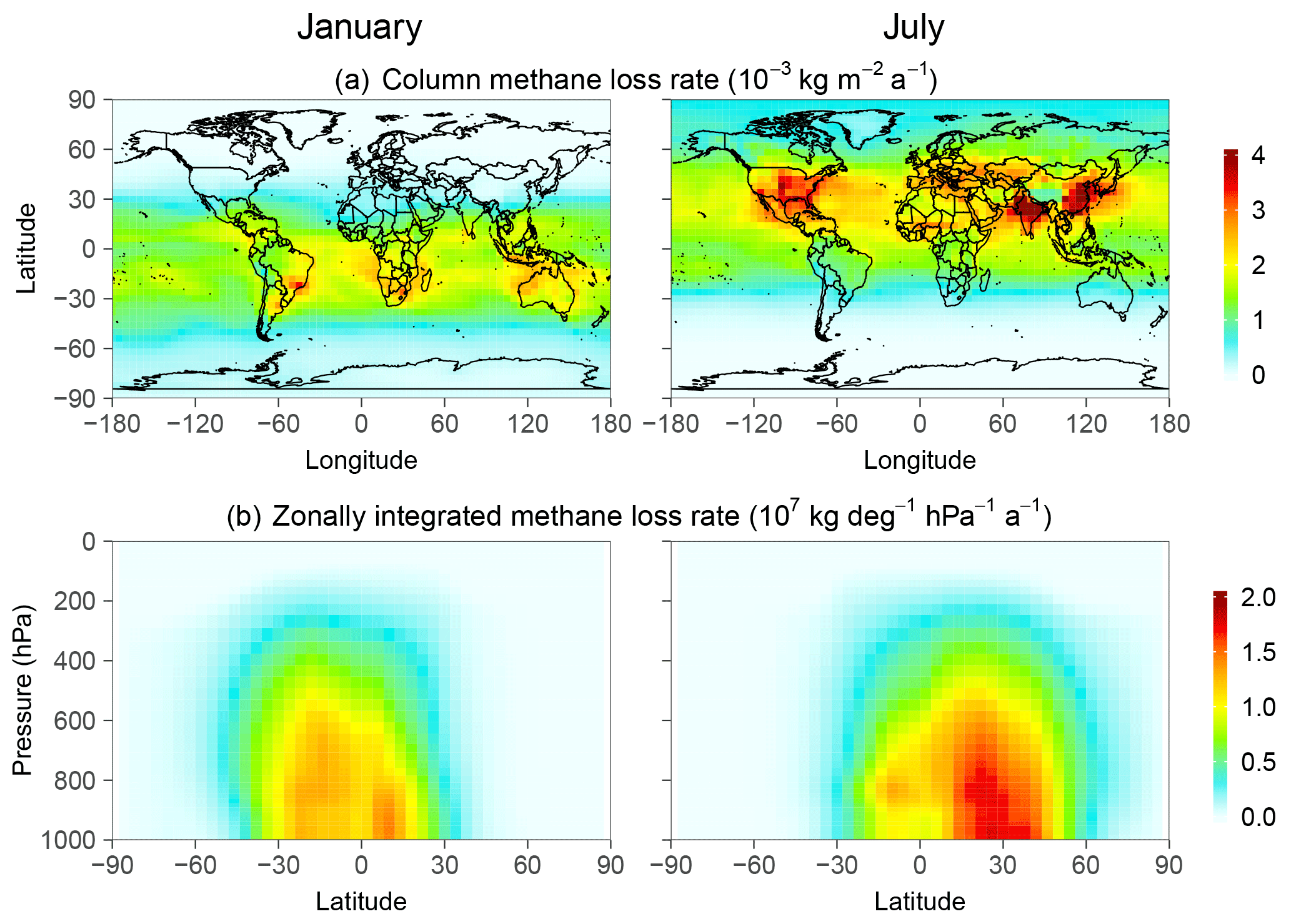
https://www.atmos-chem-phys.net/18/15959/2018/acp-18-15959-2018-f01

Figure 1Monthly methane loss rate from oxidation by OH in January and July 2015 computed with the GEOS-Chem model (Wecht et al., 2014). The top panels show the column loss rates and the bottom panels show the zonally integrated loss rates.

Download

https://www.atmos-chem-phys.net/18/15959/2018/acp-18-15959-2018-f02

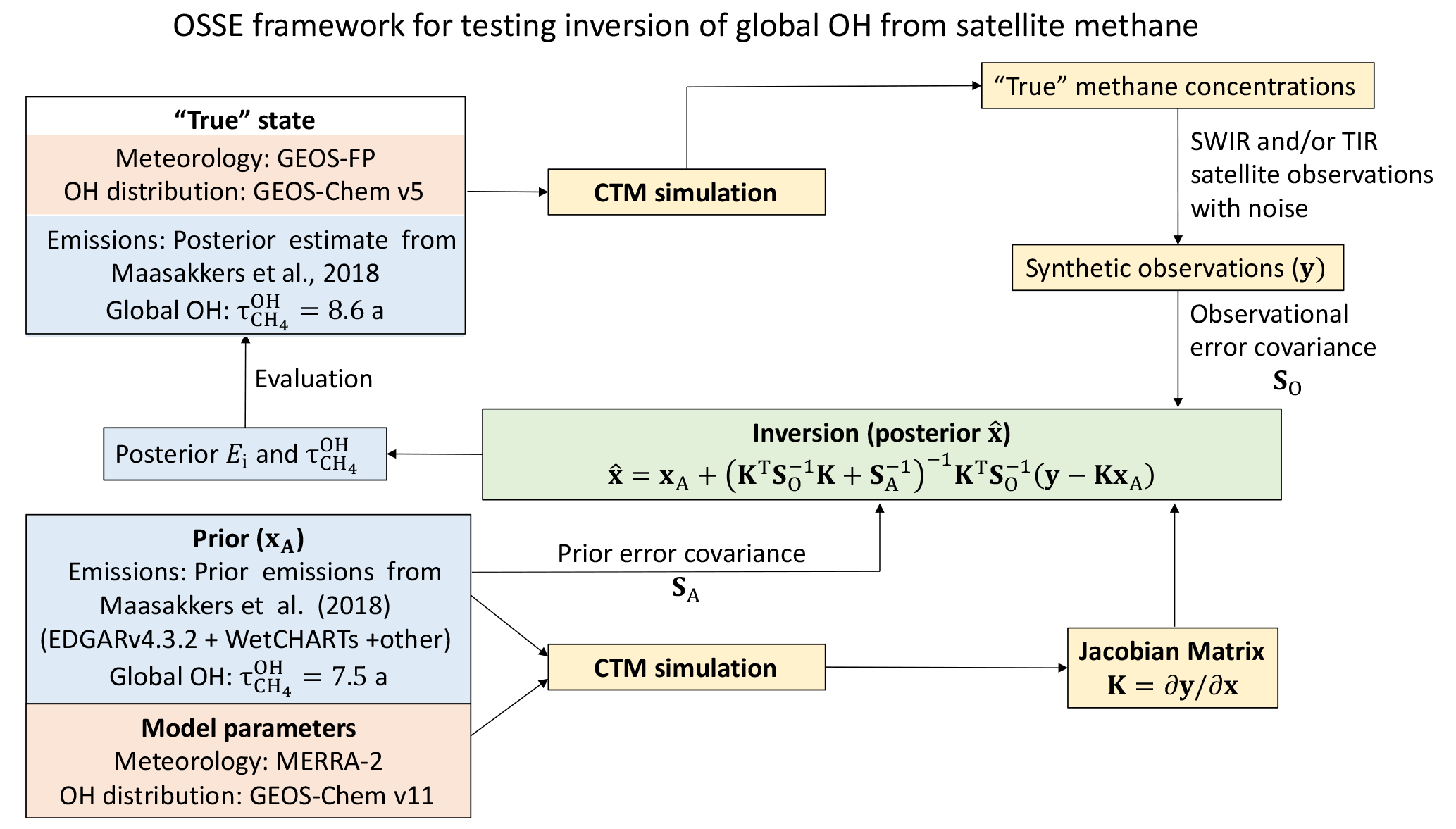
Figure 2Observing system simulation experiment (OSSE) framework to test the ability of SWIR and TIR satellite observations of atmospheric methane to simultaneously constrain methane emission rates (E_i) and the global mean tropospheric OH concentration expressed as methane lifetime against oxidation by tropospheric OH $(τ_{{CH}_{4}}^{OH})$ .

Download

Here we propose that satellite methane observations could provide a reliable proxy for global tropospheric OH, using inverse analyses that optimize OH concentrations from the satellite data alongside methane emission rates. Satellites measure methane in the short-wave infrared (SWIR, at 1.65 and 2.3 µm) by solar backscatter, and in the thermal infrared (TIR, around 7.6 µm) by terrestrial emission (Jacob et al., 2016). SWIR measurements are sensitive to the full column of methane but are mainly restricted to land, while TIR measurements are most sensitive to the middle and upper troposphere and operate over both land and ocean (Worden et al., 2015). A number of studies have used SWIR observations from the SCIAMACHY and GOSAT satellite instruments to infer methane emissions through inverse analyses. Most of these studies have assumed OH to be known (Bergamaschi et al., 2009, 2013; Spahni et al., 2011; Fraser et al., 2013, 2014; Monteil et al., 2013; Houweling et al., 2014; Alexe et al., 2015; Pandey et al., 2015; Turner et al., 2015), while a few have optimized methane emissions together with OH concentrations using methyl chloroform measurements (Cressot et al., 2014, 2016). Maasakkers et al. (2018) used 6 years of GOSAT data (2010–2015) to constrain methane emissions and their trends together with global OH trends.

Table 1OSSE conditions.

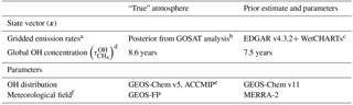
^a Methane emission rates on a $4^{\circ} \times 5^{\circ}$ grid over land excluding Antarctica (1009 elements).
^b From Maasakkers et al. (2018).
^c The prior estimate for the inversion uses anthropogenic emissions from EDGAR v4.3.2 (European Commission, 2017) except in the USA (Maasakkers et al., 2016) and oil/gas in Canada and Mexico (Sheng et al., 2017). WetCHARTs is from Bloom et al. (2017).
^d Expressed as the lifetime of a well-mixed tropospheric methane tracer against oxidation by tropospheric OH (Eq. 1).
^e Sensitivity simulations in Sect. 4 use additional 11 global OH distributions from the ACCMIP ensemble (Naik et al., 2013).
^f Meteorological fields are for 2015.

Download Print Version | Download XLSX

TIR observations are of marginal value for inversion of methane emissions because they are insensitive to the boundary layer (Wecht et al., 2012), but they could provide complementary information for constraining OH. The methane sink from oxidation by OH has a distinct atmospheric signature, peaking in the tropical troposphere, distributed zonally, and shifting seasonally with the UV flux (Fig. 1). The expected availability in the coming years of new high-density satellite data from TROPOMI in the SWIR (Hu et al., 2018) and CrIS in the TIR (Gambacorta et al., 2016) motivates the assessment of the potential of these data to provide a continuous means for monitoring global tropospheric OH concentrations.

2 Observing system simulation experiment

We conduct an observing system simulation experiment (OSSE) to examine the feasibility of inferring global tropospheric OH concentrations by inversion of satellite observations of atmospheric methane, focusing on the potential of TROPOMI and CrIS as representative of SWIR and TIR observations, respectively. The OSSE approach allows us to examine the ability of the observations to separately constrain methane emissions and OH, and to investigate the effects of errors in inversion parameters.

Figure 2 describes the structure of the OSSE. We use a chemical transport model (GEOS-Chem CTM) (Maasakkers et al., 2018) to generate a “true” (quotation marks are omitted hereafter) global 3-D time-dependent distribution of methane concentrations, given a true state defined by known 2-D monthly methane emissions and 3-D monthly OH concentrations. The true methane concentration field is sampled following the specifications of TROPOMI and CrIS to generate synthetic observations. We then use these synthetic observations in an inverse analysis system, with an independent CTM simulation and deliberately incorrect prior estimates of emissions and OH concentrations, to assess the capability of the observing system to retrieve the true state. See Brasseur and Jacob (2017) for further discussion of the OSSE approach.

The mean tropospheric OH concentration is often defined in terms of the lifetime of a long-lived gas (Prather and Spivakovsky, 1990), and in our case the natural metric is the lifetime of a well-mixed tropospheric methane tracer against oxidation by tropospheric OH:

\begin{matrix} (1) & τ_{{CH}_{4}}^{OH} = \frac{\int_{troposphere} n_{a} d v}{\int_{troposphere} k (T) [OH] n_{a} d v}, \end{matrix}

where n_a is air number density, v is volume, and $k (T) = 2.45 \times 10^{- 12} e^{- 1775 / T}$ cm³ molec⁻¹ s⁻¹ is the temperature-dependent oxidation rate constant (Burkholder et al., 2015). We will also examine interhemispheric differences in OH by integrating it over the Northern and Southern Hemisphere separately $(τ_{{CH}_{4}}^{OH, NH}$ and $τ_{{CH}_{4}}^{OH, SH})$ . An advantage of using Eq. (1) as a metric for OH is that it is independent of the atmospheric distribution of methane. Note that the integration in the numerator of Eq. (1) is over the troposphere; therefore $τ_{{CH}_{4}}^{OH}$ defined in Eq. (1) is shorter than the lifetime of total atmospheric methane against oxidation by tropospheric OH (e.g., Prather et al., 2012).

2.1 Model simulation

We use the GEOS-Chem CTM to simulate atmospheric methane concentrations in the true atmosphere and to serve as the forward model for the inversion, with different meteorological fields and OH distributions to reduce the “fraternal twin” problem (Table 1). GEOS-Chem solves the continuity equation for atmospheric methane as

\begin{matrix} (2) & \frac{\partial n}{\partial t} = - \nabla \cdot (n u) + E - k (T) n [OH] - minor sinks, \end{matrix}

where n is the methane number density, u is the wind vector, E is the emission field, and k(T) is the rate constant for reaction with OH. Minor sinks include other tropospheric sinks (reaction with the Cl atom and soil uptake) and stratospheric sinks specified as 2-D loss rate constants. The transport term $- \nabla \cdot (n u)$ not only includes advection by grid-resolved winds but also parameterized subgrid convection and boundary layer mixing. The methane simulation with GEOS-Chem v11 is as described by Wecht et al. (2014).

The GEOS-Chem simulation is conducted on a $4^{\circ} \times 5^{\circ}$ horizontal grid and 47 vertical layers (∼30 layers in the troposphere). The simulation is for year 2015 with a half-year spin-up starting from June 2014 to establish methane gradients driven by synoptic-scale transport (Turner et al., 2015). We vary the state vector elements (i.e., gridded methane emission rates and global tropospheric methane OH lifetime) between the true simulation and the inversion, to assess the ability of the inversion to retrieve the true values given synthetic observations. To include the effect of errors in model parameters that are not optimized in the inversion, we also vary the model meteorological fields (for the same meteorological year) and the monthly 3-D distribution of OH in the inversion. It should be noted that in this setup the magnitude (global mean concentration expressed as global tropospheric methane lifetime) and the distribution (seasonal and spatial variations) of the OH field are decoupled and only the former is optimized.

Table 1 summarizes the OSSE conditions. The true emissions on the $4^{\circ} \times 5^{\circ}$ grid are the posterior values from the inversion of GOSAT data by Maasakkers et al. (2018). The prior emissions include anthropogenic emissions from the EDGAR v4.3.2 global emission inventory (European Commission, 2017) replaced with Sheng et al. (2017) in Mexico and Canada for the oil and gas sector and with Maasakkers et al. (2016) in the USA, wetland emissions from WetCHARTs v1.0 (Bloom et al., 2017), and other sources (biomass burning, termite, and geological and geothermal seeps). The true global OH concentration as expressed by $τ_{{CH}_{4}}^{OH}$ is 8.6 years with spatial/seasonal OH distribution from GEOS-Chem v5, while the prior estimate is 7.5 years with distribution from GEOS-Chem v11. These OH distributions are generated from GEOS-Chem full chemistry simulations with specified methane fields based on observations, and thus are independent of the prior emissions used in the inversion. The OH distributions in GEOS-Chem v5 and v11 are significantly different due to many updates between these versions for lightning, isoprene chemistry, halogen chemistry, and emissions (Hu et al., 2017). In Sect. 4, we will consider even larger differences in OH distributions using the ACCMIP model ensemble (Naik et al., 2013).

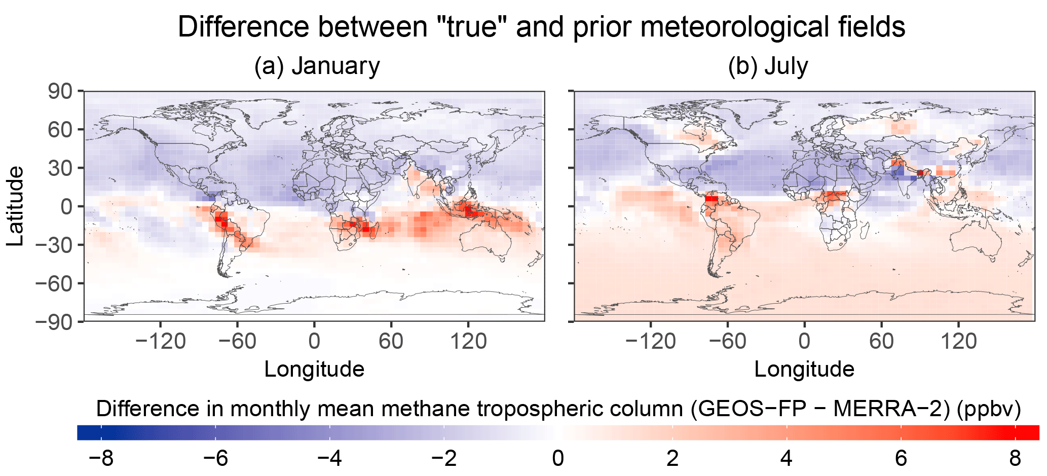
https://www.atmos-chem-phys.net/18/15959/2018/acp-18-15959-2018-f03

Figure 3Differences in monthly mean methane dry air tropospheric column mixing ratios between two simulations with different meteorological fields (GEOS-FP minus MERRA-2) for January (a) and July (b).

Download

GEOS-Chem simulations can be conducted with either of two different meteorological data sets produced by the NASA Global Modeling and Assimilation Office (GMAO): the operational Goddard Earth Observing System Forward Processing (GEOS-FP) product (Lucchesi, 2017) and the Modern-Era Retrospective analysis for Research and Applications, Version 2 (MERRA-2) (Gelaro et al., 2017). Here we use the GEOS-FP data for 2015 to produce the true methane concentrations, and the MERRA-2 data also for 2015 in the forward model for the inversion. Although GEOS-FP and MERRA-2 have commonalities, they differ in grid resolution (cubed-sphere c720 for GEOS-FP and c360 for MERRA-2), model physics (in particular convection), and level of data assimilation. This allows us to introduce some model transport errors in the OSSE. The root-mean-squared difference in daily methane tropospheric column mixing ratios between the two simulations driven by GEOS-FP and MERRA-2 (with identical emissions and OH fields) is ∼2 ppbv. Comparison of monthly mean columns between the two simulations shows patterns of differences on regional and hemispheric scales (Fig. 3), introducing a systematic component of inversion error.

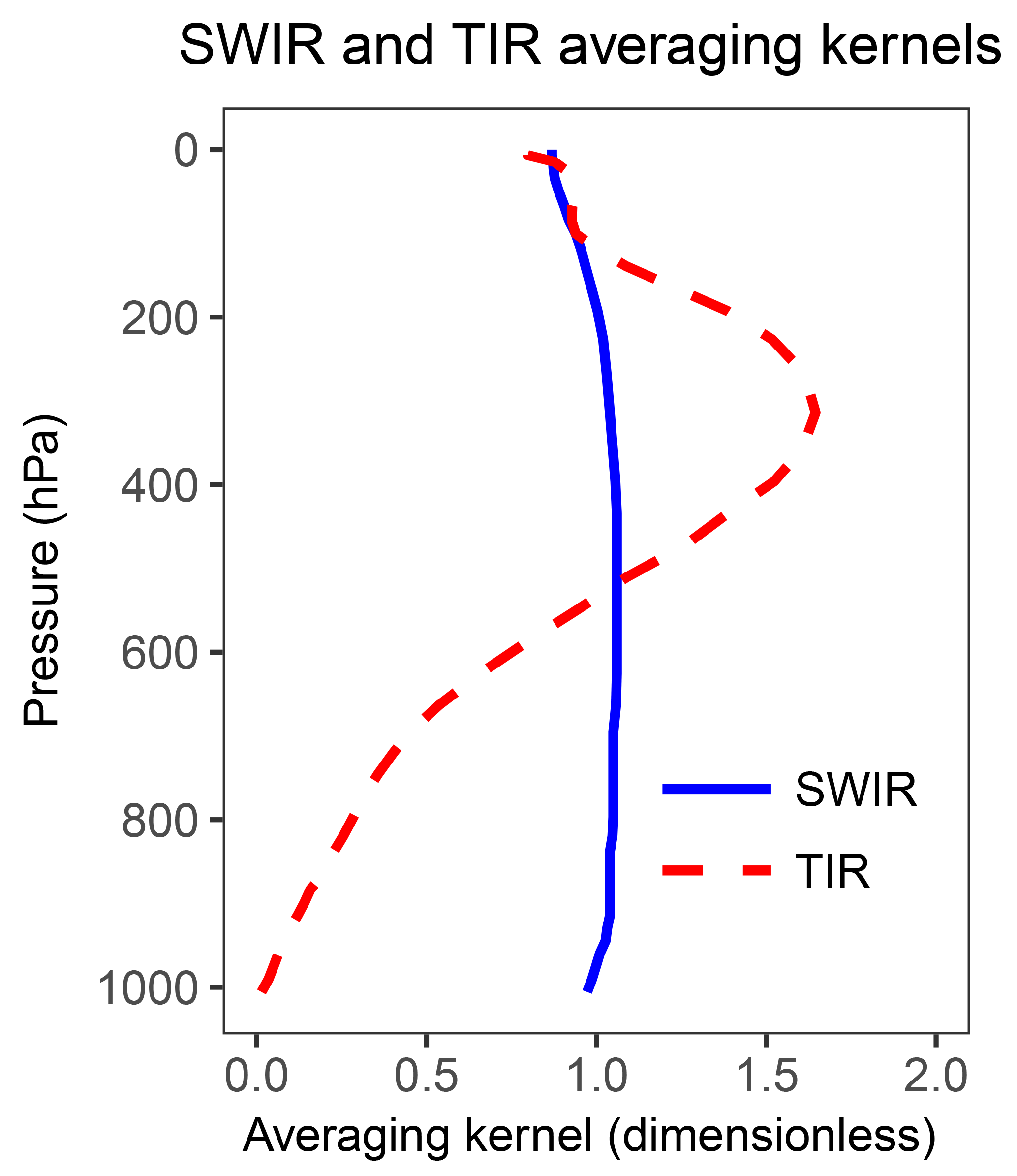
https://www.atmos-chem-phys.net/18/15959/2018/acp-18-15959-2018-f04

Figure 4Typical vertical sensitivities (column averaging kernels) for satellite observations of atmospheric methane in the SWIR and in the TIR. Adapted from Worden et al. (2015).

Download

2.2 Synthetic observations

Synthetic observations sample the true methane fields with instrument noise added (Fig. 2). For SWIR, the sampling is at local time 13:30 over land, and for TIR, at both 13:30 and 01:30 over land and ocean. The retrieval success rate (ratio between the number of successful retrievals and the number of attempted retrievals) is calculated to be 3 % for SWIR (Hu et al., 2016) and 60 % for TIR (Xiong et al., 2008) because SWIR observations require cloud-free pixels, whereas TIR has tolerance for fractional cloud cover. The retrievals are for the dry air column mixing ratio X (ppb) after applying typical averaging kernels to describe vertical sensitivity (Fig. 4). Gaussian random noise is added to the individual retrievals to simulate the instrument error, with a standard deviation of 0.6 % for SWIR TROPOMI (Butz et al., 2012) and 2 % for TIR CrIS (Gambacorta et al., 2016). To account for model biases in simulation of stratospheric methane (Patra et al., 2011) and following the recommendation of Saad et al. (2016), we replace the concentrations above 200 hPa by the 2-D seasonal climatology from ACE-FTS satellite observations (Koo et al., 2017), both in the synthetic observations and in the forward model.

The synthetic observations are sampled on the GEOS-Chem $4^{\circ} \times 5^{\circ}$ grid for the purpose of the inversion. This means that successful retrievals from individual pixels are averaged over $4^{\circ} \times 5^{\circ}$ grid cells. We assume that the noise is random and thus reduced by the square root of the number of successful retrievals (N_i,t) within grid cell i at time t. The noise will be greater if there are systematic errors in the retrievals. N_i,t is determined as the ratio between the grid cell area (A_i) and the pixel area (a), weighted by the local cloud-free fraction ( $1 - f_{i, t}$ ) taken from the true GEOS-FP meteorological fields.:

\begin{matrix} (3) & N_{i, t} = [c \times \frac{A_{i} \times (1 - f_{i, t})}{a}] . \end{matrix}

The global scaling factor c enforces the designed retrieval success rate (3 % for SWIR and 60 % for TIR). For a, we use the nadir resolution of SWIR TROPOMI (7×7 km²) and TIR CrIS (14×14 km²). The brackets [ ] represent the rounding function.

2.3 Inversion

We use the synthetic observations (assembled in an observation vector y) together with the prior estimates (x_A) and error covariance matrices for the prior (S_A) and observations (S_O) (Fig. 2) to find the analytic solution to the inverse problem. The state vector (x) that we seek to optimize consists of annual methane emission rates on a $4^{\circ} \times 5^{\circ}$ grid over land (excluding Antarctica) (1009 elements) plus either one or two elements representing the global or hemispheric methane inverse lifetimes (loss frequency).

The inverse problem presented here is not strictly linear because the loss rate depends on the methane concentration. However, a quasi-linearity can be assumed, as the range of variability of methane concentrations is sufficiently small. GEOS-Chem is therefore described for the purpose of the inversion by its Jacobian matrix $K = \partial y / \partial x$ , which relates x to y through y=Kx. We compute this Jacobian matrix explicitly by perturbing the individual terms of x and calculating the resulting changes in y with GEOS-Chem.

The observation error covariance matrix S_O is specified as a diagonal matrix summing the instrument and forward model error variances. The instrument error is computed as described in Sect. 2.2. The forward model error variance is derived with the residual error method (Heald et al., 2004). We assume no model transport error correlations on the $4^{\circ} \times 5^{\circ}$ grid. The prior error covariance matrix S_A is also specified as a diagonal matrix, assuming 50 % error standard deviation for gridded emission rates as in Maasakkers et al. (2018), and 10 % error standard deviation for the methane inverse lifetime (Naik et al., 2013). This assumes no spatial error correlation in the prior emissions on the $4^{\circ} \times 5^{\circ}$ grid, which is likely adequate for anthropogenic emissions because of the fine spatial variability of different source types (Maasakkers et al., 2016) but may not be adequate for wetlands emissions (Bloom et al., 2017). Prior emission errors can only be roughly characterized in any case.

The Bayesian cost function for the inverse problem (Brasseur and Jacob, 2017) is

\begin{array}{l} (4) & J (x) = \\ {(x - x_{A})}^{T} S_{A}^{- 1} (x - x_{A}) + γ {(y - K x)}^{T} S_{O}^{- 1} (y - K x), \end{array}

where γ is an adjustable regularization parameter to prevent overfitting to the observations (see below). An analytic solution to the J(x) minimization problem ( $d J / d x = 0$ ) yields the posterior estimate $\hat{x}$ :

\begin{matrix} (5) & \hat{x} = x_{A} + G (y - K x_{A}), \end{matrix}

where G is the gain matrix given by

\begin{matrix} (6) & G = {(γ K^{T} S_{O}^{- 1} K + S_{A}^{- 1})}^{- 1} γ K^{T} S_{O}^{- 1} . \end{matrix}

The solution also provides a closed form of the posterior error covariance matrix ( $\hat{S}$ ):

\begin{matrix} (7) & \hat{S} = {(γ K^{T} S_{O}^{- 1} K + S_{A}^{- 1})}^{- 1} . \end{matrix}

The diagonal elements of $\hat{S}$ represents the error variances of the posterior estimates $\hat{x}$ .

The need for a regularization parameter γ in Eq. (4) is because of uncertainty in the specifications of S_O and S_A, and notably the assumption that these matrices are diagonal. Here we determine based on the L-curve plot (Hansen, 2000) that γ should be in the range of 0.01–0.1 (Fig. 5a). This range of values also achieves the best agreement of the inversion with the true emissions as evaluated with the root mean square error (RMSE) (Fig. 5b). We use γ=0.05 in the subsequent analysis. The small γ value mainly results from neglecting correlations in the model transport errors; a sensitivity test in which both prior and true simulations are driven by MERRA-2 meteorology shows best performance with γ=1 for the metrics of Fig. 5b.

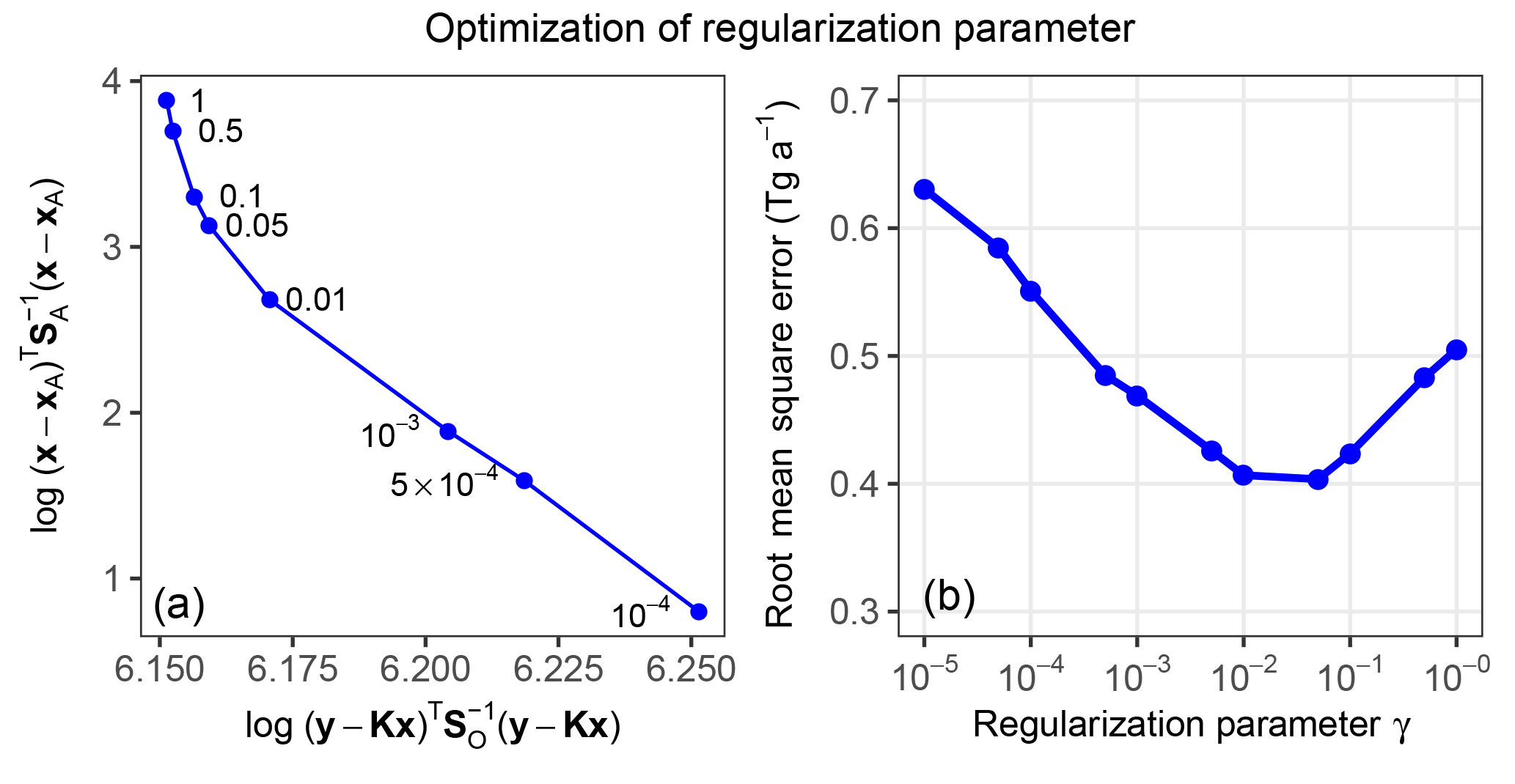
https://www.atmos-chem-phys.net/18/15959/2018/acp-18-15959-2018-f05

Figure 5Optimization of the regularization parameter γ in Eq. (4) for the SWIR + TIR satellite observing system. (a) L-curve plot (log–log plot of the squared errors of a regularized solution versus corresponding residual). Values of γ corresponding to each point are indicated. The “turning corner” of the curve indicates an optimal choice of γ (Hansen, 2000). (b) Ability of the inversion to match the true gridded methane emission field as a function of the regularization parameter. The ability is measured by the RMSE.

Download

3 Joint optimization of global

τ_{{CH}_{4}}^{OH}

and methane emission rates

Figure 6 shows the ability of the three different satellite observing systems considered here (SWIR, TIR, and SWIR + TIR) to jointly constrain gridded emission rates and $τ_{{CH}_{4}}^{OH}$ . The ability to constrain the spatial distribution of emissions is measured by the RMSE on the $4^{\circ} \times 5^{\circ}$ grid. Although all three satellite observing systems retrieve global total methane emissions within 5 % of the true value, the inversions with SWIR observations are able to resolve the distribution of methane emissions (low RMSE), while the one with only TIR observations is not (high RMSE). This is consistent with the low sensitivity of TIR to the lower troposphere (Fig. 4), where most of the information on spatially resolved emissions is contained. On the other hand, both SWIR and TIR are able to retrieve $τ_{{CH}_{4}}^{OH}$ within 3 % of the true value.

Analysis of the posterior error covariance matrix ( $\hat{S}$ ) shows that the error standard deviations σ_p on the posterior estimate of $τ_{{CH}_{4}}^{OH}$ are 0.75 %, 0.46 %, and 0.39 % for SWIR, TIR, and SWIR + TIR satellite observing systems, respectively, for a 1-year inversion (Table 2). $\hat{S}$ tends to be overoptimistic as a measure of posterior error because it assumes no systematic error in model parameters affecting the accuracy of the inversion (Brasseur and Jacob, 2017). In Sect. 4 we will explore the effect of errors in the global OH distribution as a limitation on accuracy.

Table 2Uncertainty in $τ_{{CH}_{4}}^{OH}$ estimations with different satellite observing systems.

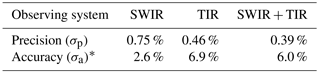
^* Accuracy is derived from inversions using different OH distributions from 12 global models for the true atmosphere (Sect. 4).

Download Print Version | Download XLSX

A central question is the ability of the inversion to independently constrain $τ_{{CH}_{4}}^{OH}$ and total emissions. The error covariance between the two can be computed from $\hat{S}$ (see Appendix for the method) and is visualized in Fig. 7. For SWIR, the significant negative correlation ( $r = - 0.78$ ) implies aliasing between corrections to OH concentration and emissions; nevertheless, the posterior error on $τ_{{CH}_{4}}^{OH}$ is greatly decreased relative to its 10 % prior value. Error correlation is less ( $r = - 0.47$ ) with the TIR observing system and the error on $τ_{{CH}_{4}}^{OH}$ is further decreased. TIR observations are more effective than SWIR for independently constraining global emissions and OH concentrations because they provide better global coverage (higher retrieval success rate) including over the oceans. The combined SWIR + TIR system has the lowest posterior errors for $τ_{{CH}_{4}}^{OH}$ , even though the error correlation with global emissions ( $r = - 0.57$ ) is greater than that for TIR only.

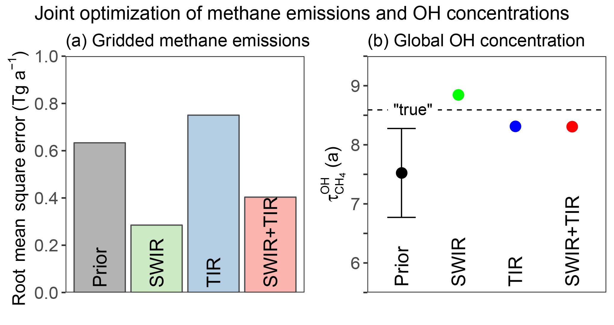
https://www.atmos-chem-phys.net/18/15959/2018/acp-18-15959-2018-f06

Figure 6Ability of SWIR, TIR, and SWIR + TIR systems to jointly constrain gridded methane emissions and global OH concentrations (as measured by the methane lifetime $τ_{{CH}_{4}}^{OH})$ in our base 1-year inversion. Panel (a) shows the RMSE in fitting the true $4^{\circ} \times 5^{\circ}$ gridded emission rates. Panel (b) compares the posterior estimates of $τ_{{CH}_{4}}^{OH}$ to the prior estimate and to the true value. The prior error standard deviation is shown as a vertical bar. Posterior error bars are too small to be shown, although this reflects overoptimistic error characterization in the inversion (see text).

Download

To go further than the error correlation analysis, we used the OSSE environment to directly test whether perturbations to OH concentrations and global emissions can be retrieved independently. We perturbed the emission rates and/or OH concentrations in three additional simulations for the true atmosphere. In the first case we increased global emissions by 10 %, in the second case we decreased global OH concentration by 5 %, and in the third case we combined both perturbations. Figure 8 shows that the posterior estimations all correctly identify the percentage changes in global total emissions and/or OH concentration, within 2 % from the true changes, in all three tests. This result further demonstrates the potential for satellite observations of methane to independently constrain global methane emissions and OH concentrations. Among all three satellite observing systems, inferred OH percentage changes with SWIR + TIR observations are closest to the true changes for all three cases, consistent with the analysis of posterior error covariance matrices (Fig. 7). The results shown in Fig. 8 suggest that satellite observations of methane should be able to detect trends in OH separately from trends in methane emissions, which has important implications for the attribution of trends in methane observations (Turner et al., 2017; Rigby et al., 2017).

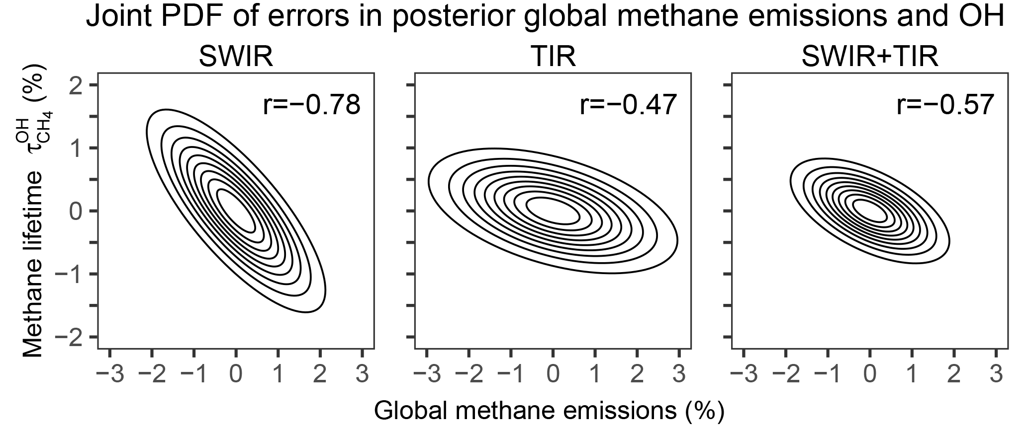
https://www.atmos-chem-phys.net/18/15959/2018/acp-18-15959-2018-f07

Figure 7Joint distribution of relative uncertainties in $τ_{{CH}_{4}}^{OH}$ and total methane emissions as given by the posterior error covariance matrices for different satellite observing systems. Contours represent confidence ellipses from probability 0.1 (innermost) to 0.9 (outermost) at an interval of 0.1. The correlation coefficients (r) between errors in $τ_{{CH}_{4}}^{OH}$ and total methane emissions are inset.

Download

4 Impact of errors in prior OH distributions

In our method, global OH abundance is represented by a single state vector element $τ_{{CH}_{4}}^{OH}$ . The seasonal and spatial distribution of OH is a forward model parameter that the inversion does not seek to optimize. Error in the prior OH distribution may therefore result in error in the posterior estimate of $τ_{{CH}_{4}}^{OH}$ that may not be fully captured by $\hat{S}$ . To test the impact of this uncertainty source, we use alternative true OH distributions from the 11 models that participated in the ACCMIP intercomparison (Naik et al., 2013), replacing the OH distribution from GEOS-Chem v5. The ACCMIP archive provides present-day (the 2000s) 3-D monthly mean OH concentrations from the different models (see Lamarque et al., 2013, for model descriptions). The ACCMIP models differ greatly in both global OH abundance and distribution (Fig. 9). To focus on errors in OH distributions, we applied a global scaling factor to each model to impose a methane lifetime $τ_{{CH}_{4}}^{OH}$ of 8.6 years, the same as in our baseline true atmosphere. To avoid complicating influence from errors in the meteorological field, we do not vary the meteorological field (i.e. MERRA-2) between the true simulation and the inversion in this test of the sensitivity to the OH distribution.

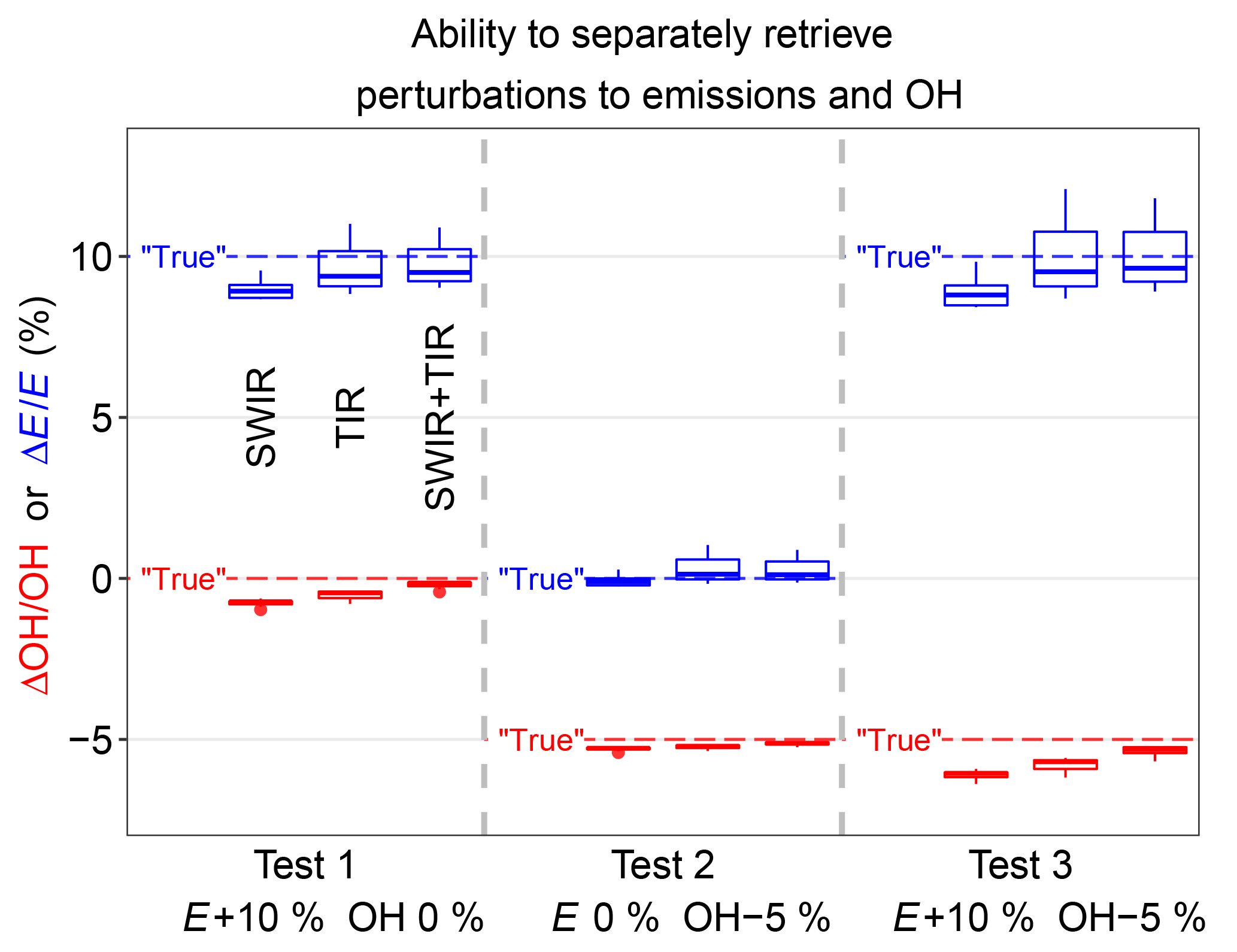
https://www.atmos-chem-phys.net/18/15959/2018/acp-18-15959-2018-f08

Figure 8OSSE experiments perturbing global emissions (E+10 %), OH (OH-5 %), and both (E+10 % OH-5 %) to test whether the inversion can retrieve these perturbations separately. Results are shown for different satellite observing systems (SWIR, TIR, and SWIR + TIR). Blue symbols represent posterior estimation of changes in emissions, and red symbols posterior estimation of change in global OH concentration. The boxes represent the 75th, 50th, and 25th percentiles, and the whiskers represent the maximum and minimum of the results using 12 different OH distributions in true simulations. Dashed lines are true changes in global emissions (blue) and OH concentration (red).

Download

Figure 10 shows the posterior estimation of $τ_{{CH}_{4}}^{OH}$ resulting from the 12 different true OH distributions (all with the same true $τ_{{CH}_{4}}^{OH}$ ). For all three satellite observing systems, the median posterior $τ_{{CH}_{4}}^{OH}$ is within 2 % of the true $τ_{{CH}_{4}}^{OH}$ . But some model OH distributions (CESM-CAM-superfast, GISS-E2-R, and CICERO-OsloCTM2) result in large errors when using TIR observations, even though they do not seem anomalous in Fig. 9. Further inspection indicates that the errors are due to large anomalies in hemispheric $τ_{{CH}_{4}}^{OH}$ ratios in boreal winter (Fig. 11), when the effect of emissions and OH on atmospheric methane is most differentiated. Errors in posterior $τ_{{CH}_{4}}^{OH}$ are smaller for SWIR only and this is because SWIR draws its information on emissions from regional patterns in concentrations, rather than the larger scale patterns in TIR. We determine the relative accuracy due to the uncertainty in the OH distribution (σ_a) as the ratio of the half interquartile range to the true $τ_{{CH}_{4}}^{OH}$ . This results in σ_a of 2.6 %, 6.9 %, and 6.0 % for SWIR, TIR, and SWIR + TIR (Table 2). Our results suggest that satellite observing systems involving TIR measurements are likely more susceptible to errors in the OH distribution for $τ_{{CH}_{4}}^{OH}$ estimations.

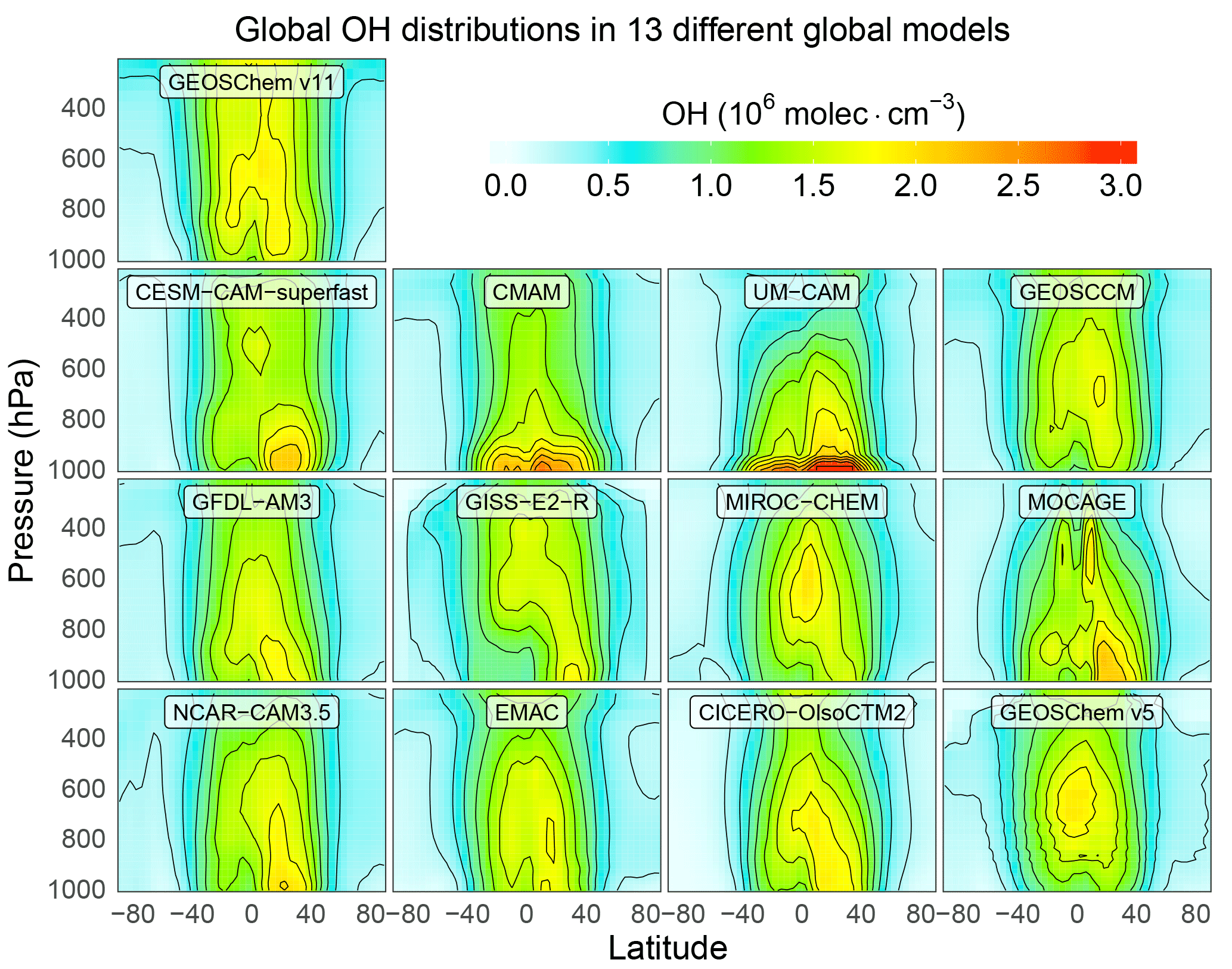
https://www.atmos-chem-phys.net/18/15959/2018/acp-18-15959-2018-f09

Figure 9Variability of OH distributions across global models. The figure shows annual zonal mean OH concentrations for 13 different models used in the OSSE. GEOS-Chem v11 is used in the forward model for the inversion with $τ_{{CH}_{4}}^{OH} = 7.5$ years. GEOS-Chem v5 is used for the baseline true atmosphere with $τ_{{CH}_{4}}^{OH} = 8.6$ years. The other 11 distributions are from the ACCMIP model ensemble (Naik et al., 2013), with global scaling factors to impose $τ_{{CH}_{4}}^{OH} = 8.6$ years in all cases, and are used in alternative representations of the true atmosphere.

Download

https://www.atmos-chem-phys.net/18/15959/2018/acp-18-15959-2018-f10

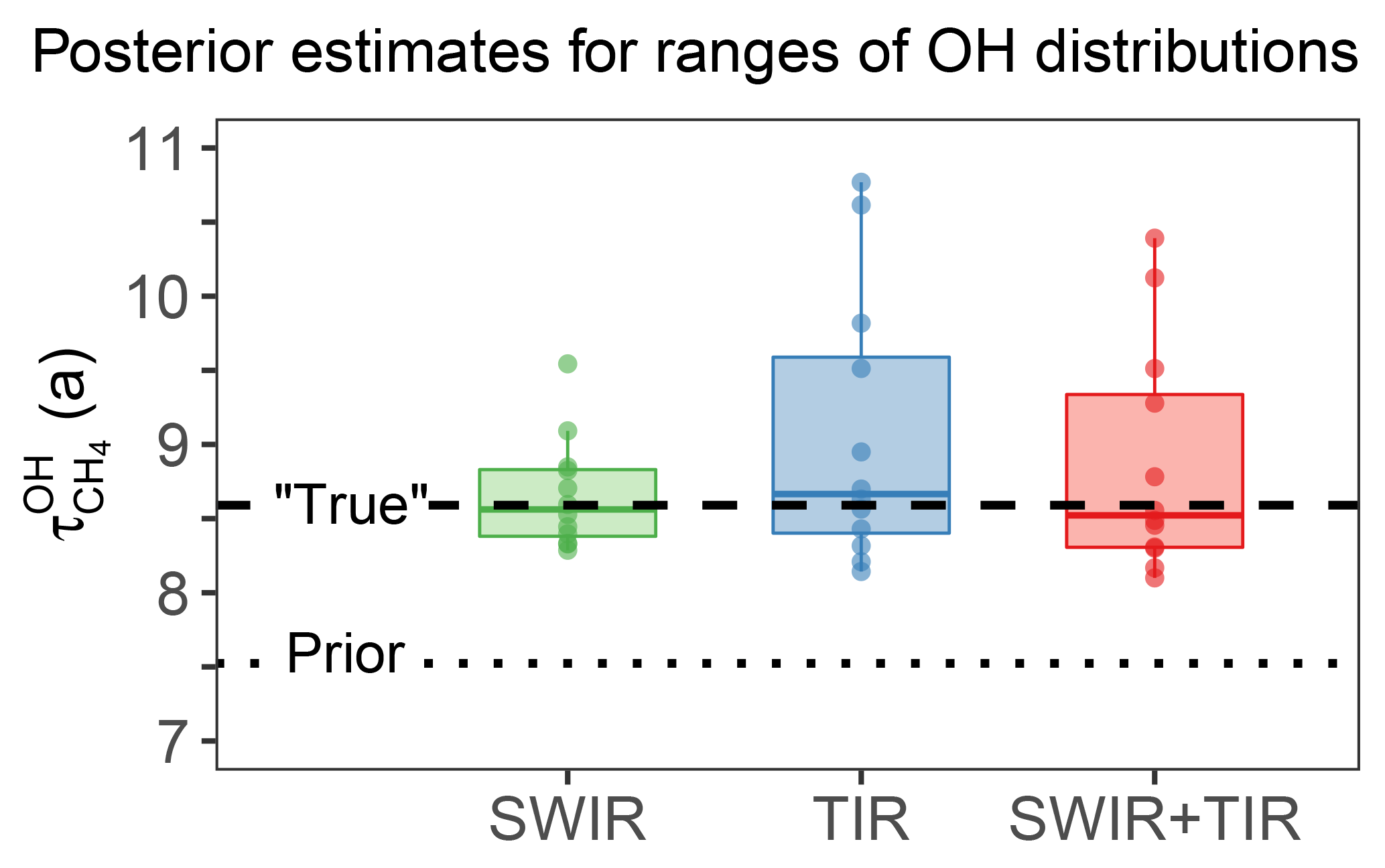
Figure 10Effect of error in OH distribution on the optimization of the global OH concentration (methane lifetime $τ_{{CH}_{4}}^{OH}$ ) from satellite observations. The figure shows the posterior estimation of $τ_{{CH}_{4}}^{OH}$ using 12 different OH distributions (Fig. 9) in simulations of the true atmosphere sampled by SWIR, TIR, and SWIR + TIR instruments, in comparison with true (dashed line) and prior (dotted line) $τ_{{CH}_{4}}^{OH}$ . The boxes represent the 75th and 25th percentiles, solid lines inside the boxes represent the medians, the whiskers represent the maximum and minimum, and dots represent results for each OH distribution.

Download

We also applied these different true OH distributions to the OSSE test of Fig. 8 perturbing emissions and/or OH to evaluate the impact of errors in OH distribution on detecting and separating changes in global $τ_{{CH}_{4}}^{OH}$ and emissions. The spread in inferred changes in OH is almost negligible for all the observing systems considered (Fig. 8), indicating that the errors resulting from imperfect OH distribution in a single-year inversion are systematic. An important implication is that these errors from imperfect OH distribution may not impair the ability to detect interannual trends in OH concentrations as long as the interannual variability in the OH distribution is relatively small.

https://www.atmos-chem-phys.net/18/15959/2018/acp-18-15959-2018-f11

Figure 11Relationship between errors in posterior estimates of $τ_{{CH}_{4}}^{OH}$ and errors in the prior $τ_{{CH}_{4}}^{OH, NH} / τ_{{CH}_{4}}^{OH,SH}$ ratio for the entire year and for boreal winter (December, January, and February). Red dots represent the three cases with large positive errors in posterior estimates of $τ_{{CH}_{4}}^{OH}$ in Fig. 10 and blue dots represent the other nine cases. The plots show that the large errors in posterior estimates of $τ_{{CH}_{4}}^{OH}$ are associated with large errors in the prior $τ_{{CH}_{4}}^{OH, NH} / τ_{{CH}_{4}}^{OH,SH}$ ratio in DJF months.

Download

The above results suggest that we may improve the estimation of $τ_{{CH}_{4}}^{OH}$ if the inversion is able to retrieve information on the OH distribution from the satellite methane observations. For this purpose, we tried to optimize the mean OH concentrations in the Northern and Southern Hemisphere separately, expressed as $τ_{{CH}_{4}}^{OH, NH}$ and $τ_{{CH}_{4}}^{OH, SH}$ . In general, the inversion is able to resolve the interhemispheric OH ratio ( $τ_{{CH}_{4}}^{OH, NH} / τ_{{CH}_{4}}^{OH, SH}$ ) for the range of OH distributions from the different global models using both SWIR and TIR satellite observing systems (Fig. 12). However, the improvement in the estimate of the global OH concentration $τ_{{CH}_{4}}^{OH}$ (computed as harmonic mean of $τ_{{CH}_{4}}^{OH, NH}$ and $τ_{{CH}_{4}}^{OH, SH}$ ) is insignificant in most cases (not shown), indicating that errors in other factors in OH distributions (e.g., vertical and seasonal distributions) in addition to the annual hemispheric ratio are also important contributors to errors in $τ_{{CH}_{4}}^{OH}$ . A careful design of the state vector that balances the resolution of OH distribution with the aliasing of OH and emissions should further improve the accuracy of the method but is beyond the scope of the current study.

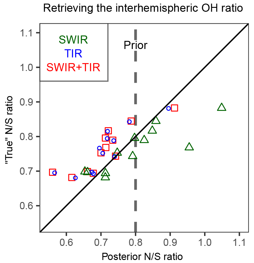
https://www.atmos-chem-phys.net/18/15959/2018/acp-18-15959-2018-f12

Figure 12Ability of the inversion of satellite methane observations to retrieve the interhemispheric OH ratio defined by $τ_{{CH}_{4}}^{OH, NH} / τ_{{CH}_{4}}^{OH,SH}$ . Posterior inversion results using SWIR, TIR, or SWIR + TIR observations are compared to the true ratio from 12 different model OH distributions (Fig. 9). The dashed vertical line represents the prior $τ_{{CH}_{4}}^{OH, NH} / τ_{{CH}_{4}}^{OH,SH}$ ratio common to all inversions.

Download

5 Conclusions

We conducted observing system simulation experiments (OSSEs) to test the feasibility of monitoring global tropospheric OH concentrations using satellite observations of methane. We considered short-wave infrared (SWIR) TROPOMI and thermal infrared (TIR) CrIS as target satellite instruments for this application, since methane retrievals from these instruments are expected to be available in the near future and will provide much improved coverage compared to current instruments. Through inversion of synthetic observations from these instruments sampling a true atmosphere, we jointly optimized gridded methane emission rates and the global tropospheric OH concentration (expressed as the lifetime of a well-mixed tropospheric methane tracer against oxidation by tropospheric OH, $τ_{{CH}_{4}}^{OH}$ as given in Eq. 1). The OSSE used different meteorological fields for the true atmosphere and for the inversion, and tested the effect of errors in the prior OH distributions.

Our results show that either SWIR or TIR observations can constrain $τ_{{CH}_{4}}^{OH}$ with a precision better than 1 %. This is an optimistic estimation of precision because we assume observational noise to be random, whereas it would have a systematic component that we cannot characterize. Nevertheless, the results show that the method has strong potential. Analysis of the posterior error covariance matrix shows that emissions and global OH concentrations can be retrieved separately because they have different signatures on the distribution of atmospheric methane. There is some error correlation, particularly for SWIR-only observations, but the posterior errors on global OH concentrations still improve considerably on the prior. Simulation experiments with perturbations to either global methane emissions and/or global OH concentration demonstrate that the method can distinguish changes in OH from changes in emissions as contributors to trends in atmospheric methane. Best performance is achieved by combining the SWIR and TIR observations. The effect of prior errors in the seasonal and spatial distributions of OH concentrations was investigated by considering global 3-D monthly concentrations fields from the 12 ACCMIP models (Naik et al., 2013), which show considerable inter-model variability. We find that these errors limit the accuracy of our method but precision is not compromised, so that interannual OH trends can still be retrieved. The effect of errors in the OH distribution could be addressed by optimizing this distribution in the state vector for the inversion, and we show that the interhemispheric OH difference at least can be successfully retrieved within ∼10 % of the true value.

We conclude that satellite observations of methane are a potentially promising alternative for methyl chloroform as a proxy for global tropospheric OH concentrations. Based on our OSSE ensemble results, we estimate the precision of the method to be 0.75 %, 0.46 %, and 0.39 % and accuracy 2.6 %, 6.9 %, and 6.0 % for SWIR, TIR, and SWIR + TIR satellite observing systems, respectively. These estimates are probably overoptimistic because of the idealized treatment of errors in the OSSE approach. The availability of TROPOMI and CrIS data will soon provide an opportunity to test the method with actual observations.

Data availability

The GEOS-Chem model is available at http://geos-chem.org (Wecht et al., 2014; last access: 15 October 2018). The ACCMIP OH distributions can be downloaded from http://catalogue.ceda.ac.uk/uuid/ded523bf23d59910e5d73f1703a2d540 (Atmospheric Chemistry and Climate Model Intercomparison Project Participants, 2011; last access: 15 October 2018). All data can be obtained from the corresponding author upon request.

Appendix A

The posterior error covariance matrix ( $\hat{S}$ ) in our inversion is a 1010×1010 matrix that characterizes the error covariance structure of gridded emission rates (E_i) in 1009 grid cells and global methane lifetime against oxidation by tropospheric OH $(τ_{{CH}_{4}}^{OH})$ . We condense $\hat{S}$ into a 2×2 matrix ${\hat{S}}_{2}$ , which represents the error covariance of global total emissions ( $E_{T} = \sum_{i = 1}^{n} E_{i}$ , where n=1009) and $τ_{{CH}_{4}}^{OH}$ :

\begin{matrix} (A1) & {\hat{S}}_{2} = [\begin{array}{ll} Var (E_{T}) & Cov (E_{T}, τ_{{CH}_{4}}^{OH}) \\ Cov (E_{T}, τ_{{CH}_{4}}^{OH}) & Var (τ_{{CH}_{4}}^{OH}) \end{array}], \end{matrix}

where $Var (τ_{{CH}_{4}}^{OH})$ is directly obtained from $\hat{S}$ , and Var(E_T) and $Cov (E_{T}, τ_{{CH}_{4}}^{OH})$ are computed from $\hat{S}$ with the following formulae:

\begin{array}{l} (A2) & Var (E_{T}) = \sum_{i = 1}^{n} Var (E_{i}) + 2 \sum_{1 \leq i < j \leq n} Cov (E_{i}, E_{j}) \\ (A3) & Cov (E_{T}, τ_{{CH}_{4}}^{OH}) = \sum_{i = 1}^{n} Cov (E_{i}, τ_{{CH}_{4}}^{OH}) . \end{array}

${\hat{S}}_{2}$ can then be visualized as a bivariate Gaussian distribution (Fig. 7).

Author contributions

YZ and DJJ designed the study. YZ performed the simulation and analysis. YZ, DJJ, JDM, JXS, RG, and JW discussed the results. JDM and DJJ initially proposed the methodology. MPS, JDM, JXS, and YZ developed the inversion system. JW provided information for CrIS specifications. YZ and DJJ wrote the paper, and JDM, JXS, RG, and JW provided input on the paper for revision before submission.

Competing interests

The authors declare that they have no conflict of interest.

Acknowledgements

This work was funded by the Interdisciplinary Science (IDS) program of the NASA Earth Science Division. Yuzhong Zhang was partially funded by the Kravis Scientific Research Fund of the Environmental Defense Fund.

Edited by: Hang Su
Reviewed by: Maarten Krol and one anonymous referee

References

Alexe, M., Bergamaschi, P., Segers, A., Detmers, R., Butz, A., Hasekamp, O., Guerlet, S., Parker, R., Boesch, H., Frankenberg, C., Scheepmaker, R. A., Dlugokencky, E., Sweeney, C., Wofsy, S. C., and Kort, E. A.: Inverse modelling of CH₄ emissions for 2010–2011 using different satellite retrieval products from GOSAT and SCIAMACHY, Atmos. Chem. Phys., 15, 113–133, https://doi.org/10.5194/acp-15-113-2015, 2015.

Bergamaschi, P., Frankenberg, C., Meirink, J. F., Krol, M., Villani, M. G., Houweling, S., Dentener, F., Dlugokencky, E. J., Miller, J. B., Gatti, L. V., Engel, A., and Levin, I.: Inverse modeling of global and regional CH₄ emissions using SCIAMACHY satellite retrievals, J. Geophys. Res.-Atmos., 114, D22301, https://doi.org/10.1029/2009JD012287, 2009.

Bergamaschi, P., Houweling, S., Segers, A., Krol, M., Frankenberg, C., Scheepmaker, R. A., Dlugokencky, E., Wofsy, S. C., Kort, E. A., Sweeney, C., Schuck, T., Brenninkmeijer, C., Chen, H., Beck, V., and Gerbig, C.: Atmospheric CH₄ in the first decade of the 21st century: Inverse modeling analysis using SCIAMACHY satellite retrievals and NOAA surface measurements, J. Geophys. Res.-Atmos., 118, 7350–7369, https://doi.org/10.1002/jgrd.50480, 2013.

Bloom, A. A., Bowman, K. W., Lee, M., Turner, A. J., Schroeder, R., Worden, J. R., Weidner, R., McDonald, K. C., and Jacob, D. J.: A global wetland methane emissions and uncertainty dataset for atmospheric chemical transport models (WetCHARTs version 1.0), Geosci. Model Dev., 10, 2141–2156, https://doi.org/10.5194/gmd-10-2141-2017, 2017.

Bousquet, P., Hauglustaine, D. A., Peylin, P., Carouge, C., and Ciais, P.: Two decades of OH variability as inferred by an inversion of atmospheric transport and chemistry of methyl chloroform, Atmos. Chem. Phys., 5, 2635–2656, https://doi.org/10.5194/acp-5-2635-2005, 2005.

Brasseur, G. P. and Jacob, D. J.: Modeling of Atmospheric Chemistry, Cambridge University Press, Cambridge, 2017.

Burkholder, J. B., Sander, S. P., Abbatt, J., Barker, J. R., Huie, R. E., Kolb, C. E., Kurylo, M. J., Orkin, V. L., Wilmouth, D. M., and Wine, P. H.: Chemical Kinetics and Photochemical Data for Use in Atmospheric Studies, Evaluation No. 18, Jet Propulsion Laboratory, Pasadena, 2015.

Butz, A., Galli, A., Hasekamp, O., Landgraf, J., Tol, P., and Aben, I.: TROPOMI aboard Sentinel-5 Precursor: Prospective performance of CH₄ retrievals for aerosol and cirrus loaded atmospheres, Remote Sens. Environ., 120, 267–276, https://doi.org/10.1016/j.rse.2011.05.030, 2012.

European Commission, Joint Research Centre (JRC)/Netherlands Environmental Assessment Agency (PBL): Emission Database for Global Atmospheric Research (EDGAR), release version 4.3.2, available at: http://edgar.jrc.ec.europa.eu/overview.php?v=432 (last access: 15 October 2018), 2017.

Cressot, C., Chevallier, F., Bousquet, P., Crevoisier, C., Dlugokencky, E. J., Fortems-Cheiney, A., Frankenberg, C., Parker, R., Pison, I., Scheepmaker, R. A., Montzka, S. A., Krummel, P. B., Steele, L. P., and Langenfelds, R. L.: On the consistency between global and regional methane emissions inferred from SCIAMACHY, TANSO-FTS, IASI and surface measurements, Atmos. Chem. Phys., 14, 577–592, https://doi.org/10.5194/acp-14-577-2014, 2014.

Cressot, C., Pison, I., Rayner, P. J., Bousquet, P., Fortems-Cheiney, A., and Chevallier, F.: Can we detect regional methane anomalies? A comparison between three observing systems, Atmos. Chem. Phys., 16, 9089–9108, https://doi.org/10.5194/acp-16-9089-2016, 2016.

Dlugokencky, E. J., Bruhwiler, L., White, J. W. C., Emmons, L. K., Novelli, P. C., Montzka, S. A., Masarie, K. A., Lang, P. M., Crotwell, A. M., Miller, J. B., and Gatti, L. V.: Observational constraints on recent increases in the atmospheric CH₄ burden, Geophys. Res. Lett., 36, L18803, https://doi.org/10.1029/2009GL039780, 2009.

Fraser, A., Palmer, P. I., Feng, L., Boesch, H., Cogan, A., Parker, R., Dlugokencky, E. J., Fraser, P. J., Krummel, P. B., Langenfelds, R. L., O'Doherty, S., Prinn, R. G., Steele, L. P., van der Schoot, M., and Weiss, R. F.: Estimating regional methane surface fluxes: the relative importance of surface and GOSAT mole fraction measurements, Atmos. Chem. Phys., 13, 5697–5713, https://doi.org/10.5194/acp-13-5697-2013, 2013.

Fraser, A., Palmer, P. I., Feng, L., Bösch, H., Parker, R., Dlugokencky, E. J., Krummel, P. B., and Langenfelds, R. L.: Estimating regional fluxes of CO2 and CH₄ using space-borne observations of XCH₄ : XCO₂, Atmos. Chem. Phys., 14, 12883–12895, https://doi.org/10.5194/acp-14-12883-2014, 2014.

Gambacorta, A., Barnet, C., Smith, N., Pierce, B., Smith, J., Spackman, R., and Goldberg, M.: The NPP and J1 NOAA Unique Combined Atmospheric Processing System (NUCAPS) for atmospheric thermal sounding: recent algorithm enhancements tailored to near real time users applications, the American Geophysical Union Fall 2016 meeting, San Francisco, California, 2016.

Gaubert, B., Worden, H. M., Arellano, A. F. J., Emmons, L. K., Tilmes, S., Barré, J., Martinez Alonso, S., Vitt, F., Anderson, J. L., Alkemade, F., Houweling, S., and Edwards, D. P.: Chemical Feedback From Decreasing Carbon Monoxide Emissions, Geophys. Res. Lett., 44, 9985–9995, https://doi.org/10.1002/2017GL074987, 2017.

Gelaro, R., McCarty, W., Suárez, M. J., Todling, R., Molod, A., Takacs, L., Randles, C. A., Darmenov, A., Bosilovich, M. G., Reichle, R., Wargan, K., Coy, L., Cullather, R., Draper, C., Akella, S., Buchard, V., Conaty, A., Silva, A. M. d., Gu, W., Kim, G.-K., Koster, R., Lucchesi, R., Merkova, D., Nielsen, J. E., Partyka, G., Pawson, S., Putman, W., Rienecker, M., Schubert, S. D., Sienkiewicz, M., and Zhao, B.: The Modern-Era Retrospective Analysis for Research and Applications, Version 2 (MERRA-2), J. Climate, 30, 5419–5454, https://doi.org/10.1175/jcli-d-16-0758.1, 2017.

Hansen, P. C.: The L-Curve and its Use in the Numerical Treatment of Inverse Problems, in: Computational Inverse Problems in Electrocardiology, edited by: Johnston, P., Advances in Computational Bioengineering, WIT Press, 119–142, 2000.

Hartmann, D. L., Klein Tank, A. M. G., Rusticucci, M., Alexander, L. V., Brönnimann, S., Charabi, Y., Dentener, F. J., Dlugokencky, E. J., Easterling, D. R., Kaplan, A., Soden, B. J., Thorne, P. W., Wild, M., and Zhai, P. M.: Observations: Atmosphere and Surface, in: Climate Change 2013: The Physical Science Basis, Contribution of Working Group I to the Fifth Assessment Report of the Intergovernmental Panel on Climate Change, edited by: Stocker, T. F., Qin, D., Plattner, G.-K., Tignor, M., Allen, S. K., Boschung, J., Nauels, A., Xia, Y., Bex, V., and Midgley, P. M., Cambridge University Press, Cambridge, United Kingdom and New York, NY, USA, 159–254, 2013.

Hausmann, P., Sussmann, R., and Smale, D.: Contribution of oil and natural gas production to renewed increase in atmospheric methane (2007–2014): top–down estimate from ethane and methane column observations, Atmos. Chem. Phys., 16, 3227–3244, https://doi.org/10.5194/acp-16-3227-2016, 2016.

Heald, C. L., Jacob, D. J., Jones, D. B. A., Palmer, P. I., Logan, J. A., Streets, D. G., Sachse, G. W., Gille, J. C., Hoffman, R. N., and Nehrkorn, T.: Comparative inverse analysis of satellite (MOPITT) and aircraft (TRACE-P) observations to estimate Asian sources of carbon monoxide, J. Geophys. Res.-Atmos., 109, D23306, https://doi.org/10.1029/2004JD005185, 2004.

Holmes, C. D., Prather, M. J., Søvde, O. A., and Myhre, G.: Future methane, hydroxyl, and their uncertainties: key climate and emission parameters for future predictions, Atmos. Chem. Phys., 13, 285–302, https://doi.org/10.5194/acp-13-285-2013, 2013.

Houweling, S., Krol, M., Bergamaschi, P., Frankenberg, C., Dlugokencky, E. J., Morino, I., Notholt, J., Sherlock, V., Wunch, D., Beck, V., Gerbig, C., Chen, H., Kort, E. A., Röckmann, T., and Aben, I.: A multi-year methane inversion using SCIAMACHY, accounting for systematic errors using TCCON measurements, Atmos. Chem. Phys., 14, 3991–4012, https://doi.org/10.5194/acp-14-3991-2014, 2014.

Hu, H., Hasekamp, O., Butz, A., Galli, A., Landgraf, J., Aan de Brugh, J., Borsdorff, T., Scheepmaker, R., and Aben, I.: The operational methane retrieval algorithm for TROPOMI, Atmos. Meas. Tech., 9, 5423–5440, https://doi.org/10.5194/amt-9-5423-2016, 2016.

Hu, H., Landgraf, J., Detmers, R., Borsdorff, T., AandeBrugh, J., Aben, I., Butz, A., and Hasekamp, O. P.: Toward global mapping of methane with TROPOMI: first results and intersatellite comparison to GOSAT, Geophys. Res. Lett., 45, 3682–3689, https://doi.org/10.1002/2018GL077259, 2018.

Hu, L., Jacob, D. J., Liu, X., Zhang, Y., Zhang, L., Kim, P. S., Sulprizio, M. P., and Yantosca, R. M.: Global budget of tropospheric ozone: Evaluating recent model advances with satellite (OMI), aircraft (IAGOS), and ozonesonde observations, Atmos. Environ., 167, 323–334, https://doi.org/10.1016/j.atmosenv.2017.08.036, 2017.

Huang, J. and Prinn, R. G.: Critical evaluation of emissions of potential new gases for OH estimation, J. Geophys. Res.-Atmos., 107, 4784, https://doi.org/10.1029/2002JD002394, 2002.

Jacob, D. J., Turner, A. J., Maasakkers, J. D., Sheng, J., Sun, K., Liu, X., Chance, K., Aben, I., McKeever, J., and Frankenberg, C.: Satellite observations of atmospheric methane and their value for quantifying methane emissions, Atmos. Chem. Phys., 16, 14371–14396, https://doi.org/10.5194/acp-16-14371-2016, 2016.

Kirschke, S., Bousquet, P., Ciais, P., Saunois, M., Canadell, J. G., Dlugokencky, E. J., Bergamaschi, P., Bergmann, D., Blake, D. R., Bruhwiler, L., Cameron-Smith, P., Castaldi, S., Chevallier, F., Feng, L., Fraser, A., Heimann, M., Hodson, E. L., Houweling, S., Josse, B., Fraser, P. J., Krummel, P. B., Lamarque, J.-F., Langenfelds, R. L., Le Quéré, C., Naik, V., O'Doherty, S., Palmer, P. I., Pison, I., Plummer, D., Poulter, B., Prinn, R. G., Rigby, M., Ringeval, B., Santini, M., Schmidt, M., Shindell, D. T., Simpson, I. J., Spahni, R., Steele, L. P., Strode, S. A., Sudo, K., Szopa, S., van der Werf, G. R., Voulgarakis, A., van Weele, M., Weiss, R. F., Williams, J. E., and Zeng, G.: Three decades of global methane sources and sinks, Nat. Geosci., 6, 813–823, https://doi.org/10.1038/ngeo1955, 2013.

Koo, J.-H., Walker, K. A., Jones, A., Sheese, P. E., Boone, C. D., Bernath, P. F., and Manney, G. L.: Global climatology based on the ACE-FTS version 3.5 dataset: Addition of mesospheric levels and carbon-containing species in the UTLS, J. Quant. Spectrosc. Ra., 186, 52–62, https://doi.org/10.1016/j.jqsrt.2016.07.003, 2017.

Krol, M. and Lelieveld, J.: Can the variability in tropospheric OH be deduced from measurements of 1,1,1-trichloroethane (methyl chloroform)?, J. Geophys. Res.-Atmos., 108, 4125, https://doi.org/10.1029/2002JD002423, 2003.

Lamarque, J.-F., Shindell, D. T., Josse, B., Young, P. J., Cionni, I., Eyring, V., Bergmann, D., Cameron-Smith, P., Collins, W. J., Doherty, R., Dalsoren, S., Faluvegi, G., Folberth, G., Ghan, S. J., Horowitz, L. W., Lee, Y. H., MacKenzie, I. A., Nagashima, T., Naik, V., Plummer, D., Righi, M., Rumbold, S. T., Schulz, M., Skeie, R. B., Stevenson, D. S., Strode, S., Sudo, K., Szopa, S., Voulgarakis, A., and Zeng, G.: The Atmospheric Chemistry and Climate Model Intercomparison Project (ACCMIP): overview and description of models, simulations and climate diagnostics, Geosci. Model Dev., 6, 179–206, https://doi.org/10.5194/gmd-6-179-2013, 2013.

Lelieveld, J., Brenninkmeijer, C. A. M., Joeckel, P., Isaksen, I. S. A., Krol, M. C., Mak, J. E., Dlugokencky, E., Montzka, S. A., Novelli, P. C., Peters, W., and Tans, P. P.: New Directions: Watching over tropospheric hydroxyl (OH), Atmos. Environ., 40, 5741–5743, https://doi.org/10.1016/j.atmosenv.2006.04.008, 2006.

Levy, H.: Normal Atmosphere: Large Radical and Formaldehyde Concentrations Predicted, Science, 173, 141–143, https://doi.org/10.1126/science.173.3992.141, 1971.

Liang, Q., Chipperfield, M. P., Fleming, E. L., Luke Abraham, N., Braesicke, P., Burkholder, J. B., Daniel, J. S., Dhomse, S., Fraser, P. J., Hardiman, S. C., Jackman, C. H., Kinnison, D. E., Krummel, P. B., Montzka, S. A., Morgenstern, O., McCulloch, A., Mühle, J., Newman, P. A., Orkin, V. L., Pitari, G., Prinn, R. G., Rigby, M., Rozanov, E., Stenke, A., Tummon, F., Velders, G. J. M., Visioni, D., and Weiss, R. F.: Deriving global OH abundance and atmospheric lifetimes for long-lived gases: A search for CH₃CCl₃ alternatives, J. Geophys. Res.-Atmos., 11914–11933, https://doi.org/10.1002/2017JD026926, 2017.

Logan, J. A., Prather, M. J., Wofsy, S. C., and McElroy, M. B.: Tropospheric chemistry: A global perspective, J. Geophys. Res.-Oceans, 86, 7210–7254, https://doi.org/10.1029/JC086iC08p07210, 1981.

Lovelock, J. E.: Methyl chloroform in the troposphere as an indicator of OH radical abundance, Nature, 267, 32–32, https://doi.org/10.1038/267032a0, 1977.

Lucchesi, R.: File Specification for GEOS-5 FP. GMAO Office Note NO. 4 (Version 1.1), 61 pp., 2017.

Maasakkers, J. D., Jacob, D. J., Sulprizio, M. P., Turner, A. J., Weitz, M., Wirth, T., Hight, C., DeFigueiredo, M., Desai, M., Schmeltz, R., Hockstad, L., Bloom, A. A., Bowman, K. W., Jeong, S., and Fischer, M. L.: Gridded National Inventory of U.S. Methane Emissions, Environ. Sci. Technol., 50, 13123–13133, https://doi.org/10.1021/acs.est.6b02878, 2016.

Maasakkers, J. D., Jacob, D. J., Sulprizio, M. P., Hersher, M., Scarpelli, T., Turner, A. J., Sheng, J., Bloom, A., Bowman, K., and Parker, R.: Global distribution of methane emissions, emission trends, and OH concentrations and trends inferred from an inversion of GOSAT satellite data for 2010–2015, in preparation, 2018.

Monks, S. A., Arnold, S. R., Emmons, L. K., Law, K. S., Turquety, S., Duncan, B. N., Flemming, J., Huijnen, V., Tilmes, S., Langner, J., Mao, J., Long, Y., Thomas, J. L., Steenrod, S. D., Raut, J. C., Wilson, C., Chipperfield, M. P., Diskin, G. S., Weinheimer, A., Schlager, H., and Ancellet, G.: Multi-model study of chemical and physical controls on transport of anthropogenic and biomass burning pollution to the Arctic, Atmos. Chem. Phys., 15, 3575–3603, https://doi.org/10.5194/acp-15-3575-2015, 2015.

Monteil, G., Houweling, S., Butz, A., Guerlet, S., Schepers, D., Hasekamp, O., Frankenberg, C., Scheepmaker, R., Aben, I., and Röckmann, T.: Comparison of CH₄ inversions based on 15 months of GOSAT and SCIAMACHY observations, J. Geophys. Res.-Atmos., 118, 11807–11823, https://doi.org/10.1002/2013JD019760, 2013.

Montzka, S. A., Krol, M., Dlugokencky, E., Hall, B., Jöckel, P., and Lelieveld, J.: Small Interannual Variability of Global Atmospheric Hydroxyl, Science, 331, 67–69, https://doi.org/10.1126/science.1197640, 2011.

Murray, L. T., Logan, J. A., and Jacob, D. J.: Interannual variability in tropical tropospheric ozone and OH: The role of lightning, J. Geophys. Res.-Atmos., 118, 11468–11480, https://doi.org/10.1002/jgrd.50857, 2013.

Myhre, G., Shindell, D., Bréon, F. M., Collins, W., Fuglestvedt, J., Huang, J., Koch, D., Lamarque, J. F., Lee, D., Mendoza, B., Nakajima, T., Robock, A., Stephens, G., Takemura, T., and Zhang, H.: Anthropogenic and natural radiative forcing, in: Climate Change 2013: The Physical Science Basis. Contribution of Working Group I to the Fifth Assessment Report of the Intergovernmental Panel on Climate Change, edited by: Stocker, T. F., Qin, D., Plattner, G. K., Tignor, M., Allen, S. K., Doschung, J., Nauels, A., Xia, Y., Bex, V., and Midgley, P. M., Cambridge University Press, Cambridge, UK, 659–740, 2013.

Naik, V., Voulgarakis, A., Fiore, A. M., Horowitz, L. W., Lamarque, J.-F., Lin, M., Prather, M. J., Young, P. J., Bergmann, D., Cameron-Smith, P. J., Cionni, I., Collins, W. J., Dalsøren, S. B., Doherty, R., Eyring, V., Faluvegi, G., Folberth, G. A., Josse, B., Lee, Y. H., MacKenzie, I. A., Nagashima, T., van Noije, T. P. C., Plummer, D. A., Righi, M., Rumbold, S. T., Skeie, R., Shindell, D. T., Stevenson, D. S., Strode, S., Sudo, K., Szopa, S., and Zeng, G.: Preindustrial to present-day changes in tropospheric hydroxyl radical and methane lifetime from the Atmospheric Chemistry and Climate Model Intercomparison Project (ACCMIP), Atmos. Chem. Phys., 13, 5277–5298, https://doi.org/10.5194/acp-13-5277-2013, 2013.

Nisbet, E. G., Dlugokencky, E. J., Manning, M. R., Lowry, D., Fisher, R. E., France, J. L., Michel, S. E., Miller, J. B., White, J. W. C., Vaughn, B., Bousquet, P., Pyle, J. A., Warwick, N. J., Cain, M., Brownlow, R., Zazzeri, G., Lanoisellé, M., Manning, A. C., Gloor, E., Worthy, D. E. J., Brunke, E. G., Labuschagne, C., Wolff, E. W., and Ganesan, A. L.: Rising atmospheric methane: 2007–2014 growth and isotopic shift, Global Biogeochem. Cy., 30, 1356–1370, https://doi.org/10.1002/2016GB005406, 2016.

Pandey, S., Houweling, S., Krol, M., Aben, I., and Röckmann, T.: On the use of satellite-derived CH₄ : CO2 columns in a joint inversion of CH₄ and CO2 fluxes, Atmos. Chem. Phys., 15, 8615–8629, https://doi.org/10.5194/acp-15-8615-2015, 2015.

Patra, P. K., Houweling, S., Krol, M., Bousquet, P., Belikov, D., Bergmann, D., Bian, H., Cameron-Smith, P., Chipperfield, M. P., Corbin, K., Fortems-Cheiney, A., Fraser, A., Gloor, E., Hess, P., Ito, A., Kawa, S. R., Law, R. M., Loh, Z., Maksyutov, S., Meng, L., Palmer, P. I., Prinn, R. G., Rigby, M., Saito, R., and Wilson, C.: TransCom model simulations of CH₄ and related species: linking transport, surface flux and chemical loss with CH₄ variability in the troposphere and lower stratosphere, Atmos. Chem. Phys., 11, 12813–12837, https://doi.org/10.5194/acp-11-12813-2011, 2011.

Prather, M. and Spivakovsky, C. M.: Tropospheric OH and the lifetimes of hydrochlorofluorocarbons, J. Geophys. Res.-Atmos., 95, 18723–18729, https://doi.org/10.1029/JD095iD11p18723, 1990.

Prather, M. J., Holmes, C. D., and Hsu, J.: Reactive greenhouse gas scenarios: Systematic exploration of uncertainties and the role of atmospheric chemistry, Geophys. Res. Lett., 39, L09803, https://doi.org/10.1029/2012GL051440, 2012.

Prinn, R. G., Huang, J., Weiss, R. F., Cunnold, D. M., Fraser, P. J., Simmonds, P. G., McCulloch, A., Harth, C., Salameh, P., Doherty, S., Wang, R. H. J., Porter, L., and Miller, B. R.: Evidence for Substantial Variations of Atmospheric Hydroxyl Radicals in the Past Two Decades, Science, 292, 1882–1888, 2001.

Rice, A. L., Butenhoff, C. L., Teama, D. G., Röger, F. H., Khalil, M. A. K., and Rasmussen, R. A.: Atmospheric methane isotopic record favors fossil sources flat in 1980s and 1990s with recent increase, P. Natl. Acad. Sci., 113, 10791–10796, https://doi.org/10.1073/pnas.1522923113, 2016.

Rigby, M., Prinn, R. G., Fraser, P. J., Simmonds, P. G., Langenfelds, R. L., Huang, J., Cunnold, D. M., Steele, L. P., Krummel, P. B., Weiss, R. F., O'Doherty, S., Salameh, P. K., Wang, H. J., Harth, C. M., Mühle, J., and Porter, L. W.: Renewed growth of atmospheric methane, Geophys. Res. Lett., 35, L22805, https://doi.org/10.1029/2008GL036037, 2008.

Rigby, M., Montzka, S. A., Prinn, R. G., White, J. W. C., Young, D., O'Doherty, S., Lunt, M. F., Ganesan, A. L., Manning, A. J., Simmonds, P. G., Salameh, P. K., Harth, C. M., Mühle, J., Weiss, R. F., Fraser, P. J., Steele, L. P., Krummel, P. B., McCulloch, A., and Park, S.: Role of atmospheric oxidation in recent methane growth, P. Natl. Acad. Sci. USA, 114, 5373–5377, https://doi.org/10.1073/pnas.1616426114, 2017.

Saad, K. M., Wunch, D., Deutscher, N. M., Griffith, D. W. T., Hase, F., De Mazière, M., Notholt, J., Pollard, D. F., Roehl, C. M., Schneider, M., Sussmann, R., Warneke, T., and Wennberg, P. O.: Seasonal variability of stratospheric methane: implications for constraining tropospheric methane budgets using total column observations, Atmos. Chem. Phys., 16, 14003–14024, https://doi.org/10.5194/acp-16-14003-2016, 2016.

Schaefer, H., Fletcher, S. E. M., Veidt, C., Lassey, K. R., Brailsford, G. W., Bromley, T. M., Dlugokencky, E. J., Michel, S. E., Miller, J. B., Levin, I., Lowe, D. C., Martin, R. J., Vaughn, B. H., and White, J. W. C.: A 21st century shift from fossil-fuel to biogenic methane emissions indicated by ¹³CH₄, Science, 352, 80–84, https://doi.org/10.1126/science.aad2705, 2016.

Sheng, J.-X., Jacob, D. J., Maasakkers, J. D., Sulprizio, M. P., Zavala-Araiza, D., and Hamburg, S. P.: A high-resolution $(0.1^{\circ} \times 0.1^{\circ}$ ) inventory of methane emissions from Canadian and Mexican oil and gas systems, Atmos. Environ., 158, 211–215, https://doi.org/10.1016/j.atmosenv.2017.02.036, 2017.

Atmospheric Chemistry and Climate Model Intercomparison Project Participants, National Centre for Atmospheric Research: Shindell, D., Zeng, G., Lamarque, J. F., Szopa, S., Nagashima, T., Naik, V., Eyring, V., and Collins, W.: The model data outputs from the Atmospheric Chemistry & Climate Model Intercomparison Project (ACCMIP), NCAS British Atmospheric Data Centre, available at: http://catalogue.ceda.ac.uk/uuid/ded523bf23d59910e5d73f1703a2d540 (last access: 15 October 2018), 2011.

Singh, H. B.: Preliminary estimation of average tropospheric HO concentrations in the northern and southern hemispheres, Geophys. Res. Lett., 4, 453–456, https://doi.org/10.1029/GL004i010p00453, 1977.

Spahni, R., Wania, R., Neef, L., van Weele, M., Pison, I., Bousquet, P., Frankenberg, C., Foster, P. N., Joos, F., Prentice, I. C., and van Velthoven, P.: Constraining global methane emissions and uptake by ecosystems, Biogeosciences, 8, 1643–1665, https://doi.org/10.5194/bg-8-1643-2011, 2011.

Turner, A. J., Jacob, D. J., Wecht, K. J., Maasakkers, J. D., Lundgren, E., Andrews, A. E., Biraud, S. C., Boesch, H., Bowman, K. W., Deutscher, N. M., Dubey, M. K., Griffith, D. W. T., Hase, F., Kuze, A., Notholt, J., Ohyama, H., Parker, R., Payne, V. H., Sussmann, R., Sweeney, C., Velazco, V. A., Warneke, T., Wennberg, P. O., and Wunch, D.: Estimating global and North American methane emissions with high spatial resolution using GOSAT satellite data, Atmos. Chem. Phys., 15, 7049–7069, https://doi.org/10.5194/acp-15-7049-2015, 2015.

Turner, A. J., Frankenberg, C., Wennberg, P. O., and Jacob, D. J.: Ambiguity in the causes for decadal trends in atmospheric methane and hydroxyl, P. Natl. Acad. Sci. USA, 114, 5367–5372, https://doi.org/10.1073/pnas.1616020114, 2017.

Voulgarakis, A., Naik, V., Lamarque, J.-F., Shindell, D. T., Young, P. J., Prather, M. J., Wild, O., Field, R. D., Bergmann, D., Cameron-Smith, P., Cionni, I., Collins, W. J., Dalsøren, S. B., Doherty, R. M., Eyring, V., Faluvegi, G., Folberth, G. A., Horowitz, L. W., Josse, B., MacKenzie, I. A., Nagashima, T., Plummer, D. A., Righi, M., Rumbold, S. T., Stevenson, D. S., Strode, S. A., Sudo, K., Szopa, S., and Zeng, G.: Analysis of present day and future OH and methane lifetime in the ACCMIP simulations, Atmos. Chem. Phys., 13, 2563–2587, https://doi.org/10.5194/acp-13-2563-2013, 2013.

Wecht, K. J., Jacob, D. J., Wofsy, S. C., Kort, E. A., Worden, J. R., Kulawik, S. S., Henze, D. K., Kopacz, M., and Payne, V. H.: Validation of TES methane with HIPPO aircraft observations: implications for inverse modeling of methane sources, Atmos. Chem. Phys., 12, 1823–1832, https://doi.org/10.5194/acp-12-1823-2012, 2012.

Wecht, K. J., Jacob, D. J., Frankenberg, C., Jiang, Z., and Blake, D. R.: Mapping of North American methane emissions with high spatial resolution by inversion of SCIAMACHY satellite data, J. Geophys. Res.-Atmos., 119, 7741–7756, https://doi.org/10.1002/2014JD021551, 2014.

Wennberg, P. O., Peacock, S., Randerson, J. T., and Bleck, R.: Recent changes in the air-sea gas exchange of methyl chloroform, Geophys. Res. Lett., 31, L16112, https://doi.org/10.1029/2004GL020476, 2004.

Worden, J. R., Turner, A. J., Bloom, A., Kulawik, S. S., Liu, J., Lee, M., Weidner, R., Bowman, K., Frankenberg, C., Parker, R., and Payne, V. H.: Quantifying lower tropospheric methane concentrations using GOSAT near-IR and TES thermal IR measurements, Atmos. Meas. Tech., 8, 3433–3445, https://doi.org/10.5194/amt-8-3433-2015, 2015.

Xiong, X., Barnet, C., Maddy, E., Sweeney, C., Liu, X., Zhou, L., and Goldberg, M.: Characterization and validation of methane products from the Atmospheric Infrared Sounder (AIRS), J. Geophys. Res.-Biogeo., 113, G00A01, https://doi.org/10.1029/2007JG000500, 2008.