the Creative Commons Attribution 4.0 License.
the Creative Commons Attribution 4.0 License.
 | 07 Nov 2018
Relationships between the planetary boundary layer height and surface pollutants derived from lidar observations over China: regional pattern and influencing factors
Tianning Su
Ralph Kahn
The frequent occurrence of severe air pollution episodes in China has been a great concern and thus the focus of intensive studies. Planetary boundary layer height (PBLH) is a key factor in the vertical mixing and dilution of near-surface pollutants. However, the relationship between PBLH and surface pollutants, especially particulate matter (PM) concentration across China, is not yet well understood. We investigate this issue at ∼1600 surface stations using PBLH derived from space-borne and ground-based lidar, and discuss the influence of topography and meteorological variables on the PBLH–PM relationship. Albeit the PBLH–PM correlations are roughly negative for most cases, their magnitude, significance, and even sign vary considerably with location, season, and meteorological conditions. Weak or even uncorrelated PBLH–PM relationships are found over clean regions (e.g., Pearl River Delta), whereas nonlinearly negative responses of PM to PBLH evolution are found over polluted regions (e.g., North China Plain). Relatively strong PBLH–PM interactions are found when the PBLH is shallow and PM concentration is high, which typically corresponds to wintertime cases. Correlations are much weaker over the highlands than the plains regions, which may be associated with lighter pollution loading at higher elevations and contributions from mountain breezes. The influence of horizontal transport on surface PM is considered as well, manifested as a negative correlation between surface PM and wind speed over the whole nation. Strong wind with clean upwind air plays a dominant role in removing pollutants, and leads to obscure PBLH–PM relationships. A ventilation rate is used to jointly consider horizontal and vertical dispersion, which has the largest impact on surface pollutant accumulation over the North China Plain. As such, this study contributes to improved understanding of aerosol–planetary boundary layer (PBL) interactions and thus our ability to forecast surface air pollution.
- Article
(4681 KB) -
Supplement
(1198 KB) - BibTeX
- EndNote


In the past few decades, China has been suffering from severe air pollution, caused by both particulate matter (PM) and gaseous pollutants. PM pollutants are of greater concern to the public, partly because they are much more visible than gaseous pollution (Chan and Yao, 2008; J. Li et al., 2016; Guo et al., 2009), and because they have discernible adverse effects on human health. Moreover, airborne particles critically impact Earth's climate through aerosol direct and indirect effects (Ackerman et al., 2004; Boucher et al., 2013; Guo et al., 2017; Kiehl and Briegleb, 1993; Z. Li et al., 2016, 2017a).
Multiple factors contribute to the severe air pollution over China. Strong emission due to rapid urbanization and industrialization is a primary cause. In addition, meteorological conditions and diffusion within the planetary boundary layer (PBL) play important roles in the exchange between polluted and clean air. Among the meteorological parameters of importance, the PBL height (PBLH) can be related to the vertical mixing, affecting the dilution of pollutants emitted near the ground through various interactions and feedback mechanisms (Emeis and Schäfer, 2006; Su et al., 2017a). Therefore, PBLH is a critical parameter affecting near-surface air quality, and it serves as a key input for chemistry transport models (Knote et al., 2015; LeMone et al., 2013). The PBLH can significantly impact aerosol vertical structure, as the bulk of locally generated pollutants tends to be concentrated within this layer. Turbulent mixing within the PBL can account for much of the variability in near-surface air quality. On the other hand, aerosols can have important feedbacks on PBLH, depending on the aerosol properties, especially their light absorption (e.g., black, organic, and brown carbon; Wang et al., 2013). Multiple studies demonstrate that absorbing aerosols tend to affect surface pollution in China through their interactions with PBL meteorology (Ding et al., 2016; Miao et al., 2016; Dong et al., 2017; Petäjä et al., 2016). In a recent comprehensive review, Li et al. (2017b) present ample evidence of such interactions and characterize their determinant factors .
There are various methods for identifying the PBLH. The gradient (e.g., Johnson et al., 2001; Liu and Liang, 2010) and Richardson number methods (e.g., Vogelezang and Holtslag, 1996) are traditional and most commonly used, both of which are typically based on temperature, pressure, humidity, and wind speed profiles obtained by radiosondes. Using fine-resolution radiosonde observations, Guo et al. (2016) obtained the first comprehensive PBLH climatology over China. Ground-based lidars, such as the micropulse lidar (MPL), are also widely used to derive the PBLH (e.g., Hägeli et al., 2000; He et al., 2008; Sawyer and Li, 2013; Tucker et al., 2009; Yang et al., 2013). The lidar-based PBLH identification relies on the principle that a temperature inversion often exists at the top of the PBL, trapping moisture and aerosols (Seibert et al., 2000), which causes a sharp decrease in the aerosol backscatter signal at the PBL upper boundary. However, using ground-based observations to retrieve the PBLH suffers from poor spatial coverage and very limited sampling. The Cloud-Aerosol Lidar with Orthogonal Polarization (CALIOP) on board the Cloud-Aerosol Lidar and Infrared Pathfinder Satellite Observations (CALIPSO) satellite (Winker et al., 2007), an operational spaceborne lidar, can retrieve cloud and aerosol vertical distributions at moderate vertical resolution, complementing ground-based PBLH measurements. Several studies already demonstrate both the effectiveness and the limitations of using CALIPSO data for PBLH detection, showing sound but highly variable agreement with those from radiosonde- and MPL-based PBLH results (Su et al., 2017b; Leventidou et al., 2013; Liu et al., 2015; Zhang et al., 2016).
Several studies have explored the relationship between PBLH and surface pollutants in China. Tang et al. (2016) used ceilometer measurements to derive long-term PBLH behavior in Beijing, further demonstrating the strong correlation between the PBLH and surface visibility under high humidity conditions. Wang et al. (2017) classified atmospheric dispersion conditions based on PBLH and wind speed, and identified significant surface PM changes that varied with dispersion conditions. Miao et al. (2017) investigated the relationship between summertime PBLH and surface PM, and discussed the impact of synoptic patterns on the development and structure of the PBL. Qu et al. (2017) derived 1-year PBLH variations from lidar in Nanjing, and identified a strong correlation between PBLH and PM, especially on hazy and foggy days.
However, the majority of studies considered data from only a few stations, and as yet, the interaction between PBLH and surface pollutants under different topographic and meteorological conditions is not well characterized. Assessing the relationship between PM and the PBLH quantitatively over the entire country is of particular interest. PBL turbulence is not the only factor affecting air quality, so there can be large regional differences in the interaction between the PBLH and PM. As such, the contributions of various factors to the PBLH–PM relationship remain uncertain, which thus warrants a further investigation.
Given the above-mentioned limitations, the current study presents a comprehensive exploration of the relationship between the PBLH and surface pollutants over China, for a wide range of atmospheric, aerosol, and topographic conditions. Since 2012, China has dramatically increased the number of instruments and implemented rigorous quality control procedures for hourly pollutant concentration measurements nationally, providing much better quality data than were previously available. The pollutant data derived from surface observations, along with CALIPSO measurements, offer us an opportunity to investigate the impact of PBLH on air quality on a nationwide basis. Regional characteristics and seasonal variations are considered. Moreover, multiple factors related to the interaction between the PBLH and PM are investigated, including surface topography, horizontal transport, and pollution level. Accounting for the influences these factors have on the relationships between PBLH and surface pollutants will help improve our understanding and forecasting capability for air pollution, as well as help refine meteorological and atmospheric chemistry models.
Table 1Description of data.
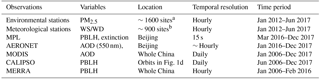
a 224 sites over the NCP; 105 sites over the PRD; 215 sites over the YRD; 159 sites over NEC. b 37 sites over the NCP; 92 sites over the PRD; 34 sites over the YRD; 76 sites over NEC.
2.1 Description of observations
2.1.1 Surface data
The topography of China is presented in Fig. 1a, and pink rectangles outline the four regions of interest (ROI) for the current study: northeast China (NEC), the Yangtze River Delta (YRD), the Pearl River Delta (PRD), and the North China Plain (NCP). The environmental monitoring station locations are indicated with red dots in Fig. 1b. They routinely measure PM with diameters ≤2.5 µm (PM2.5), which are released to the public in real time with relatively high credibility (Liang et al., 2016). The locations of meteorological stations are indicated in Fig. 1c (data source: http://data.cma.cn/en, last access: 11 January 2018). The wind speed and wind direction at these stations are quality-controlled and archived by the China Meteorological Administration. We also utilized the MPL data and Sun-photometer data in Beijing, a megacity located within the NCP. The MPL located in Beijing was operated continuously by Peking University (39.99∘ N, 116.31∘ E) from March 2016 to December 2017, with a temporal resolution of 15 s and a vertical resolution of 15 m. The near-surface blind zone for lidar is around 150 m. Background subtraction, saturation, after-pulse, overlap, and range corrections are applied to raw MPL data (He et al., 2008; Yang et al., 2013). In this study, we use Level 1.5 aerosol optical depth (AOD) at 550 nm from the Beijing RADI (40∘ N, 116.38∘ E) Aerosol Robotic Network (AERONET) site, with hourly time resolution. As observations from multiple sources and platforms are used, we present descriptions of these observations in Table 1.
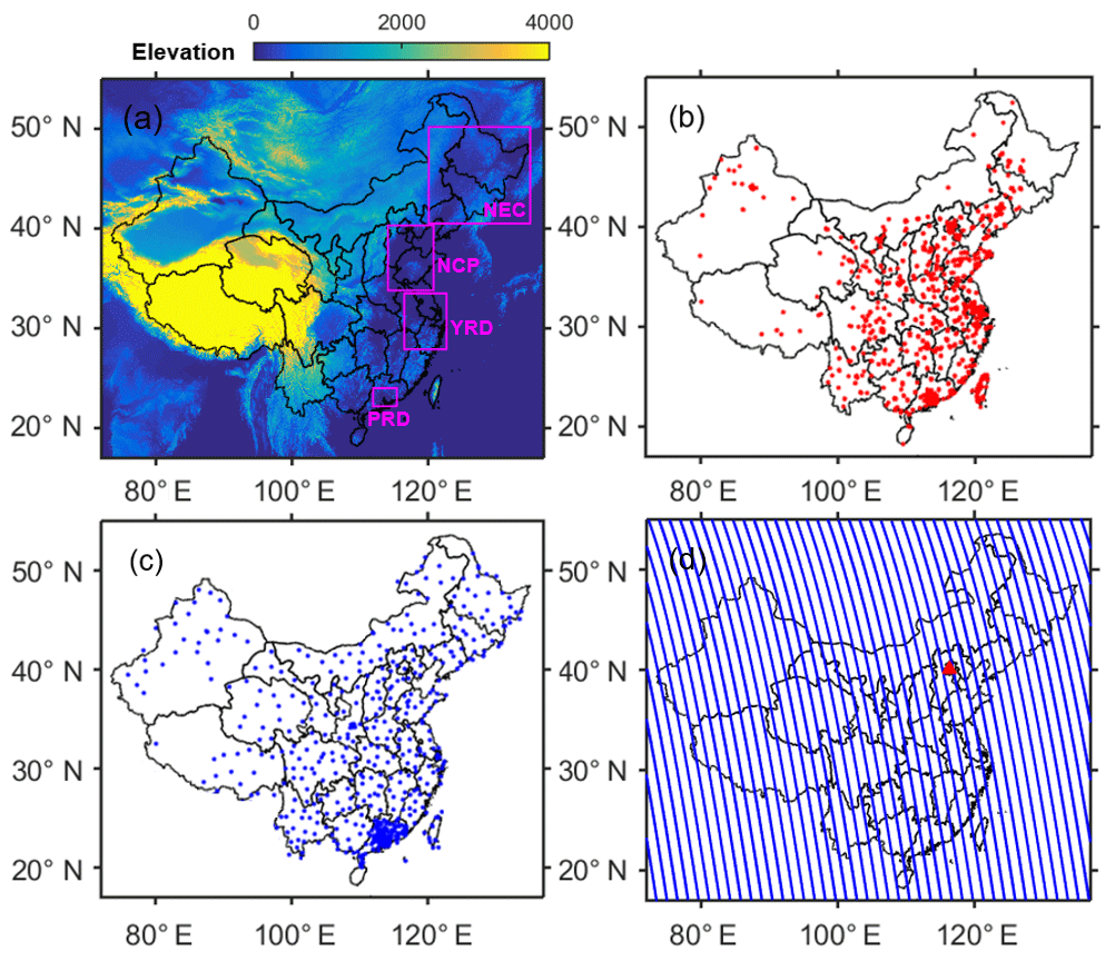
Figure 1(a) Topography of China. The black rectangles outline the five regions of interest: northeast China (NEC): 40.5–50.2∘ N, 120.1–135∘ E; North China Plain (NCP): 33.8–40.3∘ N, 114.1–120.8∘ E; Pearl River Delta (PRD): 22.2–24∘ N, 111.9–115.4∘ E; and Yangtze River Delta (YRD): 27.9–33.5∘ N, 116.5–122.7∘ E. Locations of (b) environmental stations and (c) meteorological stations. (d) Blue lines indicate CALIOP daytime orbits (in ascending node). Ground-based lidar and Sun photometer are deployed in Beijing (red triangle).
2.1.2 CALIPSO data
CALIOP aboard the CALIPSO platform is the first space-borne lidar optimized for aerosol and cloud profiling. As part of the Afternoon satellite constellation, or A-Train (L'Ecuyer and Jiang, 2010), CALIPSO is in a 705 km Sun-synchronous polar orbit between 82∘ N and 82∘ S, with a 16-day repeat cycle (Winker et al., 2007, 2009). In this study, we used the CALIPSO data to retrieve the daytime PBLH along its orbit. As shown in Fig. 1d, blue lines represent the ground tracks over China for the daytime overpasses of CALIPSO. To match the CALIPSO retrievals with equator crossings at approximately 13:30 local time, we use the surface meteorological and environmental data in the early afternoon averaged from 13:00 to 15:00 China standard time (CST). During this period, the PBL is well developed with relatively strong vertical mixing, which is a favorable condition for investigating aerosol–PBL interactions.
2.1.3 MODIS data
The MODIS instruments on board the NASA Terra and Aqua satellites have 2330 km swath widths, and provide daily AOD data with near-global coverage. In this study, we use the Collection 6 MODIS-Aqua Level-2 AOD products at 550 nm (available at: https://www.nasa.gov/langley, last access: 15 January 2018), which is a widely used parameter to represent the columnar aerosol amount. AOD data are archived with a nominal spatial resolution of 10 km × 10 km, and the data are averaged within a 30 km radius around the environmental stations to match surface PM2.5 data. The MODIS land AOD accuracy is reported to be within ± 0.05+15 % of AERONET AOD (Levy et al., 2010). Note that aerosol loading is significantly different in different regions. To account for the background pollution level, we normalize the PM2.5 with MODIS AOD to qualitatively account for background or transported aerosol that is not concentrated in the PBL.
2.2 Retrieving PBLHs
2.2.1 PBLH derived from MPL
MPL data from Beijing were used to retrieve the PBLH for this study. Multiple methods have been developed for retrieving the PBLH from MPL measurements, such as signal threshold (Melfi et al., 1985), maximum of the signal variance (Hooper and Eloranta, 1986), minimum of the signal profile derivative (Flamant et al., 1997), and wavelet transform (Cohn and Angevine, 2000; Davis et al., 2000). To derive the PBLH from MPL data, we implement a well-established method developed by Yang et al. (2013) and adopted in multiple studies (Lin et al., 2016; Su et al., 2017a, b). This method is tested to be suitable for processing long-term lidar data. Initially, the first derivative of a Gaussian filter with a wavelet dilation of 60 m is applied to smooth the vertical profile of MPL signals and to produce the gradient profile. The aerosol stratification structure is indicated by multiple valleys and peaks in the gradient profile. To exclude misidentified elevated aerosol layers above the PBL, the first significant peak in the gradient profile (if one exists) is considered the upper limit in searching for the PBL top. Then, the height of the deepest valley in the gradient profile is attributed to the PBLH; discontinuous or false results caused by clouds are subsequently eliminated manually. Moreover, we further estimated the shot noise (σ) induced by background light and dark current for each profile, and then added threshold values of ±3σ to the identified peaks and valleys of this profile to reduce the impact of noise. Figure S1 in the Supplement presents an example of the PBLH retrievals derived from MPL backscatter over Beijing. To validate MPL-derived PBLH, the values are compared with summertime radiosonde PBLH results retrieved using the Richardson number method (e.g., Vogelezang and Holtslag, 1996) from potential temperature profiles acquired at the Beijing station (39.80∘ N, 116.47∘ E) at 14:00 CST. Figure S2a shows good agreement () between MPL- and radiosonde-derived PBLHs over Beijing.
2.2.2 PBLH derived from CALIPSO
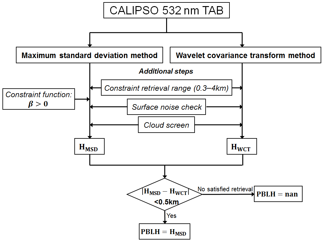
CALIOP aboard the CALIPSO platform measures the total attenuated backscatter coefficient (TAB), with a horizontal resolution of 1∕3 km and a vertical resolution of 30 m in the low and middle troposphere, and has two channels (532 and 1064 nm). As the nighttime heavy surface inversion and residual layers tend to complicate the identification of the PBLH, we only utilize daytime TAB data (Level 1B) in this study. For retrieving the PBLH from CALIPSO, we typically use the maximum standard deviation (MSD) method, which was first developed by Jordan et al. (2010) and then modified by Su et al. (2017b). In general, it determines the PBLH as the lowest occurrence of a local maximum in the standard deviation of the backscatter profile, collocated with a maximum in the backscatter itself. The PBLH retrieval range (0.3–4 km), surface noise check, and removal of attenuating and overlying clouds are subsequently included in this method. In addition, due to the viewing geometry of the instrument, we define a constraint function:
where are four adjacent altitude bins in the 532 nm TAB and where the altitude decreases with increasing bin number i. To eliminate the local standard deviation maximum caused by signal attenuation, we add the constraint β>0, and locate the PBLH at the top of the aerosol layer. We also apply the wavelet covariance transform (WCT) method to retrieve the PBLH, and this retrieval serves as a constraint. We eliminate cases when the difference between the MSD and WCT retrievals exceeds 0.5 km, to increase the reliability of the MSD retrievals. The processes and steps for retrieving PBLH from CALIPSO are summarized in Fig. 2. We only analyze CALIPSO PBLH retrievals that pass all the indicated tests and constraints. An example of PBLH retrievals derived from CALIPSO is presented in Fig. S1.
Due to the high signal-to-noise ratio and reliability of MPL measurements, we use MPL-derived PBLH to test the CALIPSO retrievals. The comparison between CALIPSO- and MPL-derived PBLH in Beijing and Hong Kong (result from Su et al., 2017b) is shown in Fig. S2b–c. Reasonable agreement between CALIPSO- and MPL-derived PBLHs at these two sites is shown. The correlation coefficients are above 0.6, which is similar to results from previous studies (e.g., Liu et al., 2015; Su et al., 2017b; Zhang et al., 2016). Besides the differences in signal-to-noise ratio, the 0–50 km distance between the MPL station and CALIPSO orbit also contributes to the differences between MPL- and CALIPSO-derived PBLH.
2.2.3 PBLH obtained from MERRA reanalysis data
We also use the PBLH data obtained from the Modern Era-Retrospective Reanalysis for Research and Applications (MERRA) reanalysis dataset to generate a PBLH climatology with a spatial resolution of 2∕3∘ × 1/2∘ (longitude–latitude). The MERRA reanalysis data use a new version of the Goddard Earth Observing System Data Assimilation System Version 5 (GEOS-5), which is a state-of-the-art system coupling a global atmospheric general circulation model (GEOS-5 AGCM) to NCEP's Grid-point Statistical Interpolation (GSI) analysis (Rienecker et al., 2011). Compared with other reanalysis products (e.g., ECMWF), MERRA PBLHs have relatively high temporal and spatial resolution, and are widely used in multiple studies (e.g., Jordan et al., 2010; McGrath-Spangler and Denning, 2012; Kennedy et al., 2011). As the reanalysis data take account of large-scale dynamical forcing, we use MERRA data to generate the PBLH climatology, which is further compared with that derived from CALIPSO in this study. A detailed discussion can be found in Sect. 3.1.
2.3 Statistical analysis methods
As a widely used parameter, the Pearson correlation coefficient derived from linear regression analysis measures the degree to which the data fit a linear relationship. This approach is less meaningful for characterizing nonlinear relationships. We find that the PBLH and PM2.5 are correlated but not linearly correlated under most conditions. We found by trial and error that an inverse function () fits our data well. Following Winship and Radbill (1994), we derived the fitting parameters (A and B) and the coefficient of determination (R2) of the PBLH–PM relationship using this inverse fitting function. Similar to the concept in the linear fitting, we define the slope in the inverse fit as A. Thus, the slope of linear fit represents the linear slope between PBLH and PM2.5, whereas the slope of an inverse fit represents the linear slope between and PM2.5. The sign of correlation coefficient for the inverse fit is the same as that of the slope. Obviously, the correlation coefficient and slope of the inverse fit for a positive relationship will be positive. Moreover, the normalized sample density at each location in a scatter plot represents the probability distribution in two dimensions (Scott, 2015). Then setting the weighting function of the inverse fit equal to the normalized density produces the best-fitting results representing the majority of cases. In general, we attempt both regular linear regression and inverse fitting to characterize the PBLH–PM relationships, and we provide the correlation coefficients and slopes for both fitting methods. In each case, the magnitude of correlation coefficient represents how well the observations are replicated by the fitting model, and the magnitude of slope represents the sensitivity of PM2.5 to PBLH changes.
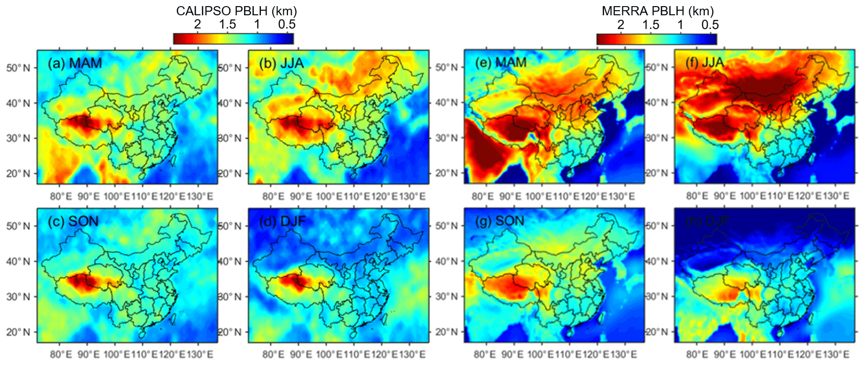
Figure 3Spatial distributions of climatological mean PBLH derived from CALIPSO for (a) March–April–May (MAM), (b) June–July–August (JJA), (c) September–October–November (SON), and (d) December–January–February (DJF) during the period 2006–2017. Spatial distributions of climatological mean of early-afternoon PBLH obtained from MERRA for (e) MAM, (f) JJA, (g) SON, and (h) DJF during the period 2006–2016.
In addition, the statistical significance of the PBLH–PM relationships is tested by two independent statistical methods, namely the least squares regression and the Mann–Kendall (MK) test (Mann, 1945; Kendall, 1975). Least squares regression typically assumes a Gaussian data distribution in the trend analysis, whereas the MK test is a nonparametric test without any assumed functional form, and is more suitable for data that do not follow a certain distribution. To improve the robustness of the analysis, a correlation is considered to be significant when the confidence level is above 99 % for both least squares regression and the MK test. Hereafter, “significant” indicates that the correlation is statistically significant at the 99 % confidence level.
3.1 Climatological patterns of PBLH and surface pollutants
The climatology of the PBLH, especially its seasonal variability, is very important for air-pollution-related studies. We utilized the CALIPSO measurements from 2006 through 2017 to represent the spatial distribution of seasonal mean PBLH with interpolation, as shown in Fig. 3a–d. A smoothing window of 20 km was applied to the original PBLH data at 1∕3 km horizontal resolution. The seasonal climatological patterns of MERRA-derived PBLH are presented in Fig. 3e–h for a similar period. In general, the climatological pattern of MERRA PBLH is similar to that of CALIPSO, though the MERRA values are higher in spring and summer, and the peak values are lower in autumn and winter. Both CALIPSO and MERRA PBLHs are generally shallower in winter, when the development of the PBL is typically suppressed by the weaker solar radiation reaching the surface, and are generally higher in summer, especially for inland regions.
Note that there are still considerable differences between the CALIPSO- and MERRA-derived PBLH climatological patterns, which can be attributed to sampling biases, different definitions, and model uncertainties. First, since the spatial coverage and time resolution are quite different between the CALIPSO and MERRA datasets, the sampling used to calculate the climatologies are quite different. Moreover, MERRA PBLHs are derived from turbulent fluxes computed by the model, whereas CALIPSO usually identifies the top height of an aerosol-rich layer. Although turbulent fluxes would significantly affect aerosol structures, the different definitions still can cause differences between CALIPSO and MERRA PBLHs. The detailed relationship between of CALIPSO- and MERRA PBLHs is presented in Fig. S2d. Quantitatively, CALIPSO PBLH values exhibit considerable differences from MERRA results; the correlation coefficient of ∼0.4 indicates that the observations presented here will likely be useful for future model refinement. The reanalysis data do take into account large-scale dynamical forcing and have the ability produce the general PBLH climatology pattern (Guo et al., 2016). However, the reanalysis data do not consider the impact of aerosols, except with limited upper atmospheric measurement data assimilated, so the effects of aerosol–PBL interactions are poorly represented (Ding et al., 2013; Simmons, 2006; Huang et al., 2018). Thus, the current reanalysis data have limited ability to support a detailed investigation of PBLH–PM relationships.
Correspondingly, Fig. 4 presents the spatial distributions of seasonal mean PM2.5 as measured at the surface stations. Both the PBLH and PM2.5 over China exhibit large spatial and seasonal variations. The PM2.5 seasonal pattern is generally coupled to that of PBLH; the lowest values occur in summer and the highest in winter. As a high PBLH facilitates the vertical dilution and dissipation of air pollution, the contrasting patterns of PBLH and PM2.5 are consistent with expectation. The NCP is a major polluted region, with mean PM2.5 concentrations overwhelmingly above 100 µg m−3 during winter. Both the PBLH and PM2.5 also show strong seasonality over the NCP. The PRD is a relatively clean region, and PM2.5 maintains low values (<50 µg m−3) through all seasons. As a reference, the seasonal means and standard deviations of PBLH and PM2.5 over four ROIs are listed in Table S1 in the Supplement.
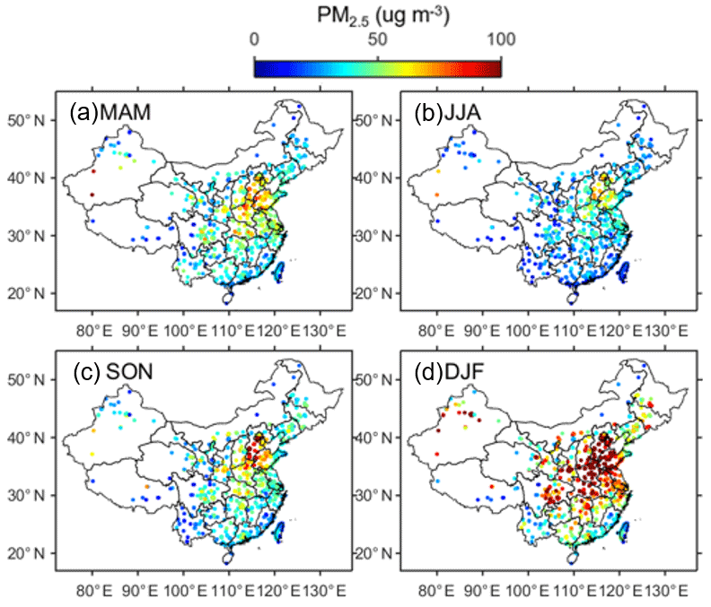
Figure 4Spatial distributions of climatological mean of early-afternoon PM2.5 concentration (in µg m−3) for (a) MAM, (b) JJA, (c) SON, and (d) DJF during the period 2012–2017.
From the seasonal climatologies, we find a coupling pattern between PBLH and PM2.5, although one cannot assume a causal relationship from these plots alone. In subsequent sections, we use the lidar PBLH retrievals to investigate the PBLH–PM relationships in more detail.
3.2 Regional relationships between PM and PBLH
If the common factor driving large-scale variations in both PM and PBLH is meteorology, a regional analysis of their relationship could elucidate the meteorological impacts. We investigate the CALIPSO PBLH and surface PM2.5 data case by case. By matching the available CALIPSO retrievals within 35 km of the surface PM2.5 observations, we show the scatter plots for PBLH versus surface PM2.5 for the four ROIs in Fig. 5. Despite the overall negative correlations, the correlations between PBLH and PM2.5 have large spreads and differences. Both regular linear regression and inverse fitting are applied to characterize the PBLH–PM relationships. Significant negative correlations between PM2.5 and PBLH are found over the NCP, with a Pearson correlation coefficient of −0.36. In addition, the nonlinear inverse function shows high consistency with the average values for each bin, and characterizes the PBLH–PM relationship with a somewhat higher correlation coefficient (−0.49). PBLH also shows significant negative correlation with PM2.5 over the YRD and NEC, whereas the weak PBLH correlation with PM2.5 over the PRD is not statistically significant. The correlation coefficients for the inverse fit are generally larger than the Pearson correlation coefficients, indicating that the nonlinear fit may be more suitable for characterizing the PBLH–PM relationships. Such improvements are obvious for the NCP and the YRD, but are not significant over the PRD and NEC.
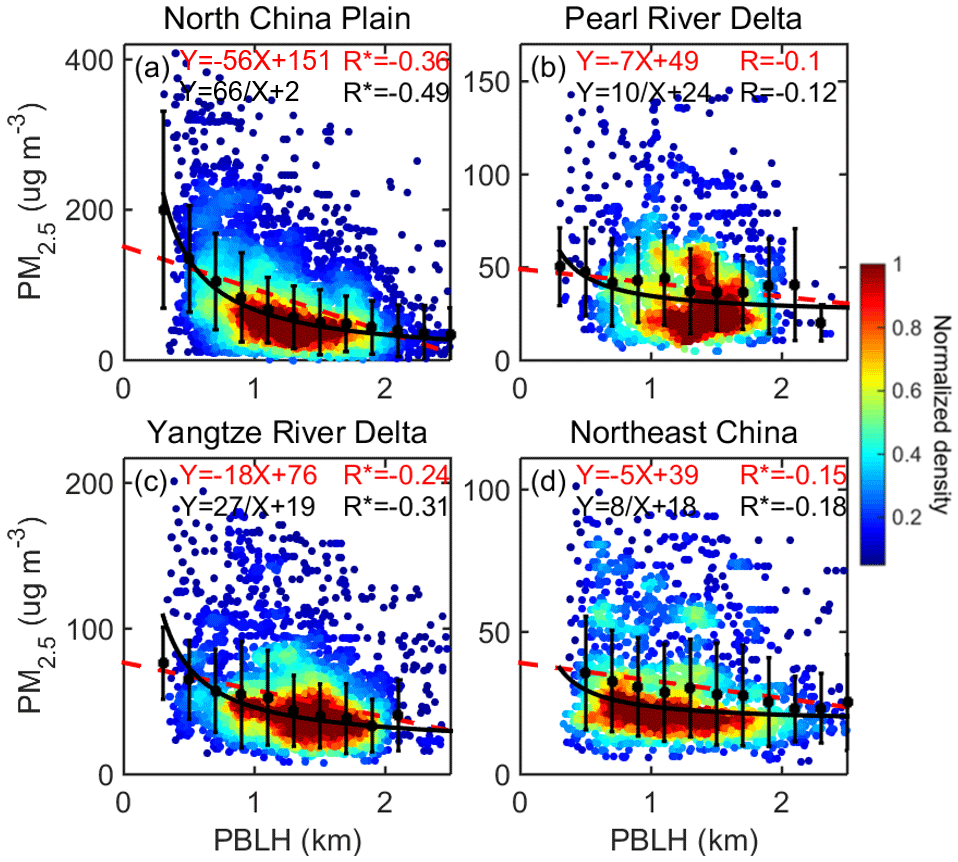
Figure 5The relationship between CALIPSO-derived PBLH and early-afternoon PM2.5 over (a) the NCP, (b) the PRD, (c) the YRD, and (d) NEC. The black dots and whiskers represent the average values and standard deviations for each bin. The red dashed lines indicate the regular linear regressions, and the black lines represent the inverse fit (). The detailed fitting functions are given at the top of each panels, along with the Pearson correlation coefficient (red) and the correlation coefficient for the inverse fit (black). Here and in the following analysis, R with asterisks indicates that the correlation is statistically significant at the 99 % confidence level. The color-shaded dots indicate the normalized sample density.
We note that the ranges of PM2.5 for these ROIs are significantly different; therefore, the background pollution level is likely to be an important factor for the PBLH–PM relationship. We thus normalize the PM2.5 by MODIS AOD, a widely used parameter to represent the total-column aerosol amount, to qualitatively account for background or transported aerosol that is not concentrated in the PBL. The relationships between PBLH and PM2.5/AOD over four ROIs are presented in Fig. 6. Clearly, after normalizing PM2.5 by AOD, the spread of these scatter plots and the regional differences are significantly reduced, and the correlations become more significant for all ROIs, especially for the PRD. This is because transported aerosol aloft can contribute to variability in total-column AOD that is unrelated to the PBLH.

Figure 6Similar to Fig. 5, but for the relationship between CALIPSO PBLH and early-afternoon PM2.5/AOD (unit: µg m−3 per AOD) over the four ROIs. Here, the AOD data are obtained from MODIS.
Compared to CALIPSO data, the MPL has a much higher signal-to-noise ratio and can continuously observe at one location. Therefore, Fig. 7 shows the relationship between MPL-derived PBLH and PM2.5 over Beijing (a major city in the NCP), as well as the relationship between PBLH and normalized PM2.5. We find the PBLH–PM relationships derived from MPL over Beijing are similar to those derived from CALIPSO over the NCP. Probably because of higher data quality, the correlation coefficients for both fitting methods are slightly higher for the relationships derived from surface observations than those from CALIPSO. Consistent with the results over the NCP, the PBLH shows a significantly nonlinear relationship with PM2.5 over Beijing. As the inverse fitting method better characterizes the PBLH–PM relationships than the regular linear fitting, we only use the inverse fitting method for the PBLH–PM relationships in the main text.
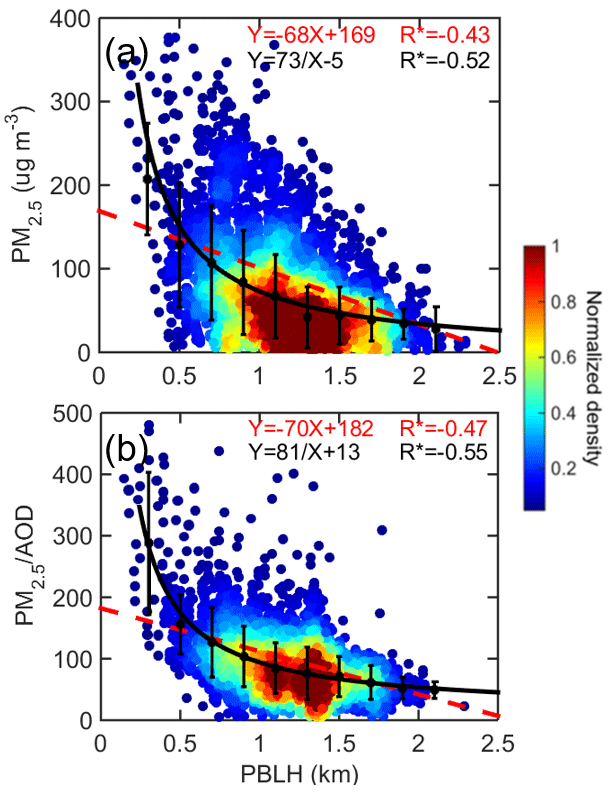
Figure 7(a) Relationship between MPL-derived PBLH and PM2.5 over Beijing. (b) Relationship between MPL-derived PBLH and PM2.5/AOD (unit: µg m−3 per AOD) over Beijing. The AOD data are obtained from AERONET. Here, linear (red) and inverse fits (black) are both shown. We only include data acquired during 10:00–15:00 local time, when the PBL is well developed.
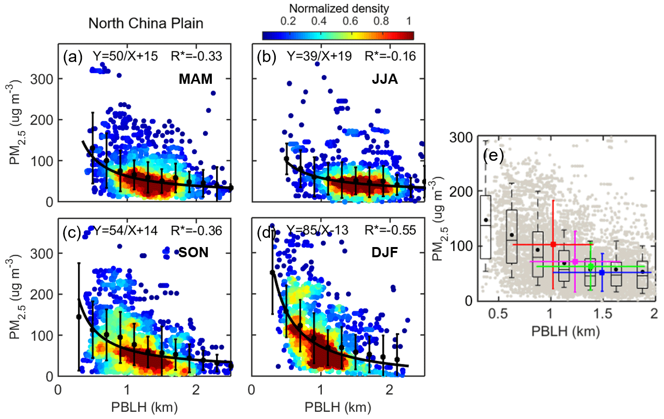
Figure 8The relationship between CALIPSO PBLH and PM2.5 over the NCP for (a) MAM, (b) JJA, (c) SON, and (d) DJF. (e) General relationship between PM2.5 and PBLH aggregated over all seasons, with individual observations for each day plotted as gray dots. The box-and-whisker plots showing 10th, 25th, 50th, 75th, and 90th percentile values of PM2.5 for each bin. The green, blue, pink, and red dots present the mean values for MAM, JJA, SON, and DJF, respectively.
The most negative correlations between PBLH and PM2.5 appear over the NCP, likely a testament to intense PBL–aerosol interactions, which may be caused by concentrated local sources. Comparing with southeast China, absorbing aerosol loading is much greater over the NCP, and may have strong interaction with the PBL through a positive feedback (Dong et al., 2017), which may contribute to the significant nonlinear relationships over the NCP. Note that the PBLH–PM2.5 correlations are apparently stronger for heavily polluted regions than for clean regions. However, after normalizing PM2.5 by AOD, the correlations are improved preferentially for clean regions (where aerosol aloft makes a larger fractional contribution to the total AOD), and thus, the differences between clean and polluted regions are reduced (Fig. S3). It further indicates that the background pollution level plays a critical role in interpreting the PBLH–PM observations.
As the NCP experiences the most pronounced seasonality in both PBLH and PM2.5, the relationship over this region also shows the most prominent seasonal differences (Fig. S4). Figure 8 focuses on the seasonal dependence of the PBLH and PM2.5 relationship over the NCP. The magnitude of the slope between 1∕PBLH and PM2.5 for this region is ∼90 (unit: km µg m−3), with a correlation coefficient of −0.55 during winter, and only ∼40 in summer. For comparison, the seasonally aggregated relationship between PBLH and PM2.5 is presented in Fig. 8e. PM2.5 concentrations do not increase linearly with decreasing PBLH. Specifically, PM2.5 increases rapidly with decreasing PBLH when PBLH is lower than 1 km, but changes much more slowly for PBLH >1.5 km. The seasonal mean values for PM2.5 and PBLH are presented as colored dots in Fig. 8e, and the whiskers represent the standard deviations. For winter, the PBLH is generally shallow and PM2.5 concentrations are high, and thus PBLH shows the most significant negative correlation with PM2.5. Conversely, in summer, the PBLH is generally higher, PM2.5 concentrations are lower, and the PBLH–PM2.5 relationship is virtually flat. Such seasonally distinct PBLH–PM2.5 relationships have not previously been studied quantitatively, and have the potential for improving PM2.5 monitoring and predictions.
3.3 Association with horizontal transport
The PBLH mainly affects the vertical mixing and dispersion of air pollution, but horizontal transport also plays a critical role in surface air quality. Figure 9a–b present the PBLH–PM2.5 relationships over China under strong wind (WS > 4 m s−1) and weak wind (WS < 4 m s−1) conditions. Under strong wind conditions, PM2.5 is found to be much less sensitive to PBLH than for weak wind. In addition, Fig. 9c–d show the aerosol extinction profiles as a function of PBLH under strong and weak wind conditions, as retrieved by the MPL in Beijing, with the Klett method applied (Klett, 1985). In both strong and weak wind conditions, we find clear aerosol extinction gradients at the top of the PBL. Nonetheless, under strong wind, the aerosol extinction is typically low in the PBL, and the surface extinction does not change significantly with different PBLHs. In this situation, the strong wind likely plays a dominant role in affecting PM2.5 concentration by ventilating the PBL. Under weak wind, the response of near-surface pollutants to PBLH is more nonlinear, and both aerosol extinction and PM2.5 fall rapidly as the PBLH increases from 600 to 1200 m.
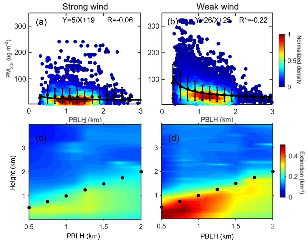
Figure 9The relationship between CALIPSO PBLH and PM2.5 over China for (a) strong wind (WS > 4 m s−1) and (b) weak wind (WS < 4 m s−1). The aerosol extinction profiles at ∼550 nm derived from the MPL in Beijing change with different MPL-derived PBLHs under (c) strong wind and (d) weak wind conditions. In (c) and (d), the black dots indicate the location of the PBL top.
We further consider the relationship between PBLH and PM2.5 under different wind direction regimes for Beijing. Two different regimes are easy to identify: a northerly wind and a southerly wind; these are divided by the red line in Fig. 10a. The northerly air comes from arid and semiarid regions in northwest China and Mongolia, and is usually strong and clean. The southerly wind comes from the southern part of the NCP, with high humidity and aerosol content. To relate the connections between WS, PBLH, and surface air quality, at least qualitatively, the ventilation rate (VR) can be represented as VR = WS × PBLH (Tie et al., 2015). Figure 10b–c and d–e present the PBLH–PM2.5 and VR–PM2.5 relationships under southerly wind and northerly wind conditions, respectively. For all wind conditions, the VR shows a reciprocal relationship with surface PM2.5. Under northerly wind conditions, both PBLH–PM2.5 and VR–PM2.5 relationships are flatter and have lower correlation coefficients. The northerly wind is apparently effective in removing pollutants and may play a dominant role in affecting air quality. For the southerly wind, the PM2.5 concentration is highly sensitive to PBLH and VR values.
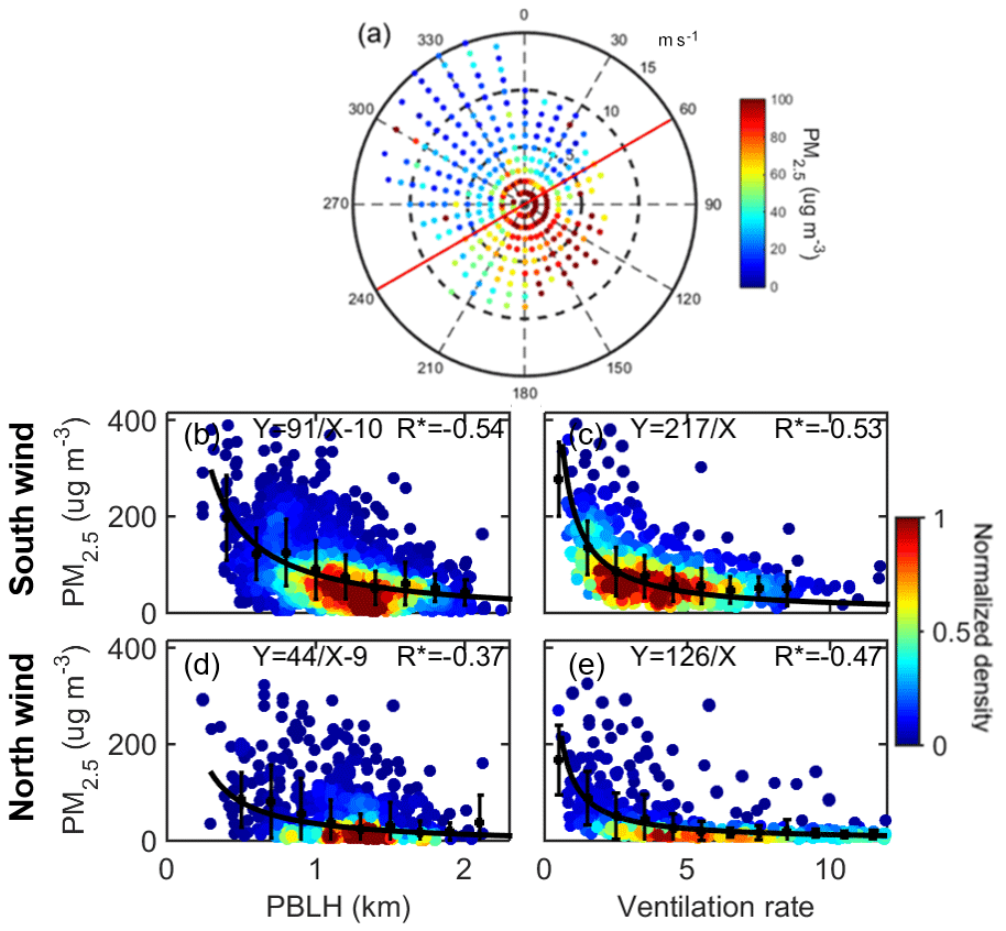
Figure 10(a) Relationship between wind direction/wind speed and PM2.5 over Beijing. The red line divides the northerly wind and southerly wind regimes. (b–c) The relationship between PM2.5 and MPL-PBLH/ventilation rate (VR = WS×PBLH, unit: km m s−1), for southerly winds over Beijing. (d–e) The relationship between PM2.5 and MPL-PBLH/VR, for northerly winds over Beijing.
To further illustrate the coupling effects of PBLH and WS on surface pollutants, Fig. 11a presents the relationship between early-afternoon WS and PM2.5 concentration across China. Overall, WS is negatively correlated with PM2.5, although a few stations over southwest China show positive correlations. A negative correlation might be expected in general, as strong winds can be effective at removing air pollutants; however, other factors such as wind direction must also be considered, as, for example, upwind sources could increase pollution under higher wind conditions. There are positive correlations between PBLH and near-surface WS in most cases (Fig. S5a), and thus, low PBLH and weak WS tend to occur together over much of China. These unfavorable meteorological conditions for air quality would exacerbate severe pollution episodes.

Figure 11(a) Spatial distribution of linear correlation coefficients (R) for the WS–PM2.5 relationship. (b) Spatial distribution of fitting parameter (A) for the VR–PM2.5 relationship. The function is used to characterize the relationship between VR and PM2.5, with A (unit: km µg m−3) as the fitting parameter. Both WS and PM2.5 are obtained from surface data, and PBLH is derived from CALIPSO. Here and in the following analysis, dots marked with black circles indicate where the relationship is statistically significant at the 99 % confidence level.
To consider horizontal and vertical dispersion jointly, we investigate the nationwide relationships between the VR and PM2.5. In general, the VR is overwhelmingly negative correlated with surface PM2.5 (Fig. S5b). Based on Fig. 10, the VR is typically reciprocal to PM2.5 for different wind conditions, and thus, we use the function to characterize the relationship between the VR and PM2.5, with A as the fitting parameter. The spatial distribution of A, presented in Fig. 11b, shows the largest values over the NCP, indicating that the PM2.5 concentration is highly sensitive to the VR there. Moreover, VRs are relatively large over the coastal areas, where sea–land breezes could play a role in dispersing air pollution. The detailed relationships and fitting functions for four ROIs are presented in Fig. S6. We note that although there are large regional differences in the PBLH–PM2.5 relationship (Fig. 5), the VR–PM2.5 relationships are similar for the different study regions. Therefore, by combining vertical and horizontal dispersion conditions, the overall VR apparently has a similar effect on PM2.5 for all four ROIs.
3.4 Correlations with topography
The PBL structure and PM2.5 concentration can both be affected by topography. We divided the sites into two categories based on elevation: plains (elevation < 0.5 km) and highlands (elevation > 1 km). Figure 12a–d present the correlation coefficients and slopes in the inverse fit between PM2.5 and PBLH for the plains and highland areas. For calculating the correlation coefficient and slope, we require that the number of matched CALIPSO PBLH and PM2.5 samples is larger than 15 for each site. Much higher correlation coefficients are found in the plains than the highlands, and the slope (i.e., linear slopes between and PM2.5) in the plains is ∼3 times that in the highlands. A reciprocal relationship is shown between station elevation and the slope between and PM2.5 (Fig. 12e). The magnitudes of slopes decrease dramatically with elevation increase, for elevations between 0 and 500 m. Local emissions also affect aerosol loading, and differences between plains and highland areas regarding local source activity could be important here as well. Figure 12e shows that the low-elevation regions are typically more polluted than highland areas, and the magnitudes of the slopes tend to be higher. Here, we utilized the inverse fitting method to reveal the different PBLH–PM relationships for the plains and highland areas, and we reach a similar conclusion by using the linear fitting method (Fig. S7).
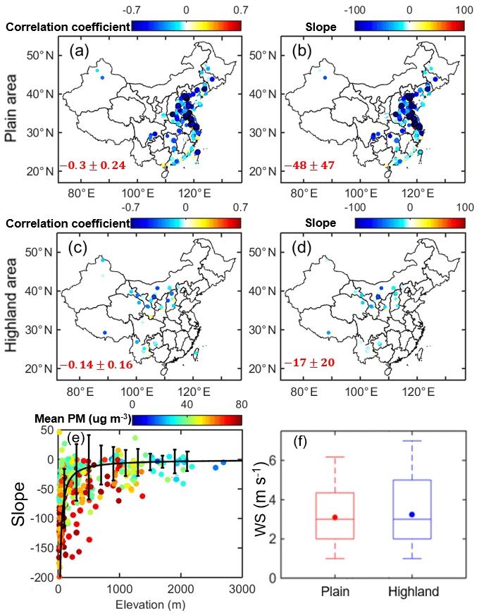
Figure 12Stratification by terrain elevation. The correlation coefficients (R) and slopes (unit: km µg m−3) between CALIPSO PBLH and PM2.5 for the inverse fit () are shown for the (a–b) plains and (c–d) highland areas. Note the slope in the inverse fit is defined as A. (e) The slopes of the inverse fit (i.e., linear slopes between and PM2.5) under different station elevations, with color shading indicating station mean PM2.5 concentration. (f) Box-and-whisker plots showing the 10th, 25th, 50th, 75th, and 90th percentile values of the early-afternoon WS for plain and highland regions. The dots indicate the mean values.
Returning to Fig. S3, stronger correlations for PBLH–PM2.5 relationships are found over polluted regions, which also correspond to the plains areas, due to strong local emissions. Therefore, high aerosol loading is likely to be another factor contributing to the strong correlation between PBLH and PM2.5 over the plains, whereas the low PM2.5 concentration may contribute to the weak PBLH–PM2.5 correlation over the highlands.
In addition, horizontal transport is associated with topography. Thus, we illustrate the distribution of WS for plains and highland areas in Fig. 12f. WS is generally larger for highland areas, especially for the strongest wind cases. In fact, the 10 % and 25 % quantiles of WS are nearly the same between plains and highland areas, whereas there are clear differences in the 75 % and 90 % quantiles. Strong wind cases account for 37% of the total over highland areas, but only 27 % of the total over the plains. As discussed in Sect. 3.3, strong wind can effectively remove surface pollutants, and can play a dominant role in determining local pollution levels. In this situation, PBLH might not play as critical a role in PM2.5 concentration. Thus, mountain winds, along with less local emission, are likely to be leading factors accounting for the differences in PBLH–PM2.5 correlations between plains and highland areas.
Other factors could come into play as well, such as the vertical distribution of aerosol, the insolation, and the actual single-scattering albedo of the particles; further examination of these phenomena is beyond the scope of the current paper.
Based on 10 years of CALIPSO measurements and other environmental data obtained from more than 1500 stations, large-scale relationships between PBLH and PM2.5 are assessed over China. Although the PBLH–PM2.5 correlations are generally negative for the majority of conditions, the magnitude, significance, and even sign vary greatly with location, season, and meteorological conditions. Nonlinear responses of PM2.5 to PBLH evolution are found under some conditions, especially for the NCP, the most polluted region of China. We further applied an inverse function () to characterize the PBLH–PM2.5 relationships, with overall better performance than a linear regression. The nonlinear relationship between PBLH and PM2.5 shows stronger interaction when the PBLH is shallow and PM2.5 concentration is high, which typically corresponds to the wintertime cases. Specifically, the negative correlation between PBLH and PM2.5 is most significant during winter. Moreover, we find that regional differences in the PBLH–PM2.5 relationships are correlated with topography. The PBLH–PM2.5 correlations are found to be more significant in low-altitude regions. This might be related to the more frequent air stagnation and strong local emission over China's plains, as well as a greater concentration of emission sources. The mountain breezes and a larger fraction of transported aerosol above the PBL contribute to weakening of the PBLH–PM2.5 correlation over highland areas.
Note that the PBLH–PM2.5 relationships are not always significant, nor are they always negative (Geiß et al., 2017). In addition to PBLH, PM2.5 is also affected by other factors, such as emissions, wind, synoptic patterns, and atmospheric stability. In some situations (e.g., strong wind and low aerosol loading), PBLH does not play a dominant role in modulating surface pollutants, and this results in weak or uncorrelated relationships between PBLH and PM2.5. Weak PBLH–PM2.5 correlations are a common feature over relatively clean regions. Due to the importance of regional pollution levels, we normalized PM2.5 by MODIS total-column AOD to account for the background aerosol in different regions. Compared to PBLH–PM2.5 correlations, the correlations between PBLH and normalized PM2.5 (PM2.5/AOD) increased significantly for clean regions, resulting in smaller regional differences overall. The retrieval of surface PM2.5 from AOD constraints has been investigated in many studies. The detailed relationships between PBLH and PM2.5/AOD over different ROIs are also expected to be significant for relating PM2.5 to remotely sensed AOD, due to the way PBLH affects near-surface aerosol concentration.
Horizontal transport also shows significant inverse correlation with PM2.5 concentrations. WS and PBLH tend to be positively correlated in the study regions, which means meteorologically favorable horizontal and vertical dispersion conditions are likely to occur together. Wind direction can also significantly affect the PBLH–PM2.5 relationship. Strong wind with clean upwind sources plays a dominant role in improving air quality over Beijing, for example, and leads to weak PBLH–PM2.5 correlation. The combination of WS and PBLH, representing a ventilation rate (VR), shows a reciprocal correlation with surface PM2.5 in all the regions studied. The VR is also found to have the largest impact on surface pollutant accumulation over the NCP.
The feedback of absorbing aerosol is also a potential factor affecting the PBLH–PM2.5 relationships. Compared with southeast China (e.g., PRD), absorbing aerosol loading is much higher over the NCP, and is reported to have strong interaction with the PBL via a positive feedback in this region (Dong et al., 2017; Ding et al., 2016; Huang et al., 2018). Such conclusions are consistent with our results, which show significant PBLH–PM2.5 correlations over the NCP and weak correlations over the PRD. The important feedback of absorbing aerosols may also contribute to the nonlinear relationship between PBLH and PM2.5. This issue merits further analysis using comprehensive measurements from field experiments, from which integrated aerosol conditions and model simulations can account for aerosol radiative forcing while controlling for the other relevant variables.
Our work comprehensively covers the relationships between PBLH and surface pollutants over large regional spatial scales in China. Multiple factors, such as background pollution level, horizontal transport, and topography, are found to be highly correlated with PBLH and near-surface aerosol concentration. Such information can help improve our understanding of the complex interactions between air pollution, boundary layer depth, and horizontal transport, and thus, can benefit policymaking aimed at mitigating air pollution at both local and regional scales. Our findings provide deeper insight and contribute to the quantitative understanding of aerosol–PBL interactions, which could help in refining meteorological and atmospheric chemistry models. Further, this work may enhance surface pollution monitoring and forecasting capabilities.
The meteorological data are provided by the Data Center of the China Meteorological Administration (data link: http://data.cma.cn/en, last access: 11 January 2018). The hourly PM2.5 data are released by the Ministry of Environmental Protection of the People's Republic of China (data link: http://113.108.142.147:20035/emcpublish, last access: 12 January 2018) and Taiwan Environmental Protection Administration (data link: http://taqm.epa.gov.tw, last access: 12 January 2018). The CALIPSO and MODIS data are obtained from the NASA Langley Research Center Atmospheric Science Data Center (data link: https://www.nasa.gov/langley, last access: 15 January 2018). The MERRA reanalysis data are publicly available at https://disc.sci.gsfc.nasa.gov/datasets?page=1&keywords=merra (last access: 7 December 2017). The AERONET data are publicly available at https://aeronet.gsfc.nasa.gov (last access: 5 July 2018).
The supplement related to this article is available online at: https://doi.org/10.5194/acp-18-15921-2018-supplement.
ZL and TS conceptualized this study. TS carried out the analysis, with comments from other co-authors. TS, ZL, and RK interpreted the data and wrote the manuscript.
The authors declare that they have no conflict of interest.
This article is part of the special issue “Regional transport and transformation of air pollution in eastern China”. It is not associated with a conference.
This study has been supported in part by the National Science Foundation (NSF) of China (91544217), National Key R&D
Project of China (2017YFC1501702), and the US NSF (AGS1534670). The authors would like to
acknowledge the Department of Atmospheric and Oceanic Sciences of Peking
University for providing the ground-based lidar data. We thank Chengcai Li
and Jing Li for theirs effort in establishing and maintaining the MPL site.
We thank Zhengqiang Li for his effort in establishing and maintaining the
Beijing RADI AERONET site. We greatly appreciate the helpful advice from
Jing Li and Chengcai Li at Peking University. We acknowledge the provision of
surface pollutant data by the Ministry of Environmental Protection of the
People's Republic of China and Taiwan Environmental Protection
Administration, and also acknowledge the provision of meteorological data by the China
Meteorological Administration. We extend sincerest thanks to the CALIPSO,
MODIS, and MERRA teams for their datasets. The contributions of Ralph Kahn
are supported in part by NASA's Climate and Radiation Research and Analysis
Program under Hal Maring and NASA's
Atmospheric Composition Modeling and Analysis Program under
Richard Eckman.
Edited by: Yuan Wang
Reviewed by: Shuyan Liu
and two anonymous referees
Ackerman, A. S., Kirkpatrick, M. P., Stevens, D. E., and Toon, O. B.: The impact of humidity above stratiform clouds on indirect aerosol climate forcing, Nature, 432, 1014–1017, https://doi.org/10.1038/nature03174, 2004.
Boucher, O., Randall, D., Artaxo, P., Bretherton, C., Feingold, G., Forster, P., Kerminen, V. M., Kondo, Y., Liao, H., Lohmann, U., and Rasch, P.: Clouds and aerosols, in: Climate Change 2013: The Physical Science Basis. Contribution of Working Group I to the Fifth Assessment Report of the Intergovernmental Panel on Climate Change, 571–657, Cambridge Univ. Press, Cambridge, UK and New York, NY, USA, 2013.
Chan, C. K. and Yao, X.: Air pollution in megacities in China, Atmos. Environ., 42, 1–42, https://doi.org/10.1016/j.atmosenv.2007.09.003, 2008.
Cohn, S. A. and Angevine, W. M.: Boundary layer height and entrainment zone thickness measured by lidars and wind-profiling radars, J. Appl. Meteorol., 39, 1233–1247, https://doi.org/10.1175/1520-0450(2000)039<1233:BLHAEZ>2.0.CO;2, 2000.
Davis, K. J., Gamage, N., Hagelberg, C. R., Kiemle, C., Lenschow, D. H., and Sullivan P. P.: An objective method for deriving atmospheric structure from airborne lidar observations. J. Atmos. Ocean. Tech., 17, 1455–1468, https://doi.org/10.1175/1520-0426(2000)017<1455:AOMFDA>2.0.CO;2, 2000.
Ding, A. J., Fu, C. B., Yang, X. Q., Sun, J. N., Petäjä, T., Kerminen, V.-M., Wang, T., Xie, Y., Herrmann, E., Zheng, L. F., Nie, W., Liu, Q., Wei, X. L., and Kulmala, M.: Intense atmospheric pollution modifies weather: a case of mixed biomass burning with fossil fuel combustion pollution in eastern China, Atmos. Chem. Phys., 13, 10545–10554, https://doi.org/10.5194/acp-13-10545-2013, 2013.
Ding, A. J., Huang, X., Nie, W., Sun, J. N., Kerminen, V.-M., Petäjä, T., Su, H., Cheng, Y. F., Yang, X.-Q., Wang, M. H., Chi, X. G., Wang, J. P., Virkkula, A., Guo, W. D., Yuan, J., Wang, S. Y., Zhang, R. J., Wu, Y. F., Song, Y., Zhu, T., Zilitinkevich, S., Kulmala, M., and Fu, C. B.: Enhanced haze pollution by black carbon in megacities in China, Geophys. Res. Lett., 43, 2873–2879, https://doi.org/10.1002/2016GL067745, 2016.
Dong, Z., Li, Z., Yu, X., Cribb, M., Li, X., and Dai, J.: Opposite long-term trends in aerosols between low and high altitudes: a testimony to the aerosol–PBL feedback, Atmos. Chem. Phys., 17, 7997–8009, https://doi.org/10.5194/acp-17-7997-2017, 2017.
Emeis, S. and Schäfer, K.: Remote sensing methods to investigate boundary-layer structures relevant to air pollution in cities, Bound.-Lay. Meteorol., 121, 377–385, 2006.
Flamant, C., Pelon, J., Flamant, P. H., and Durand, P.: Lidar determination of the entrainment zone thickness at the top of the unstable marine atmospheric boundary layer, Bound.-Lay. Meteorol., 83, 247–284, https://doi.org/10.1023/A:1000258318944, 1997.
Geiß, A., Wiegner, M., Bonn, B., Schäfer, K., Forkel, R., von Schneidemesser, E., Münkel, C., Chan, K. L., and Nothard, R.: Mixing layer height as an indicator for urban air quality?, Atmos. Meas. Tech., 10, 2969–2988, https://doi.org/10.5194/amt-10-2969-2017, 2017.
Guo, J., Miao, Y., Zhang, Y., Liu, H., Li, Z., Zhang, W., He, J., Lou, M., Yan, Y., Bian, L., and Zhai, P.: The climatology of planetary boundary layer height in China derived from radiosonde and reanalysis data, Atmos. Chem. Phys., 16, 13309–13319, https://doi.org/10.5194/acp-16-13309-2016, 2016.
Guo, J., Su, T., Li, Z., Miao, Y., Li, J., Liu, H., Xu, H., Cribb, M., and Zhai, P.: Declining frequency of summertime local-scale precipitation over eastern China from 1970 to 2010 and its potential link to aerosols, Geophys. Res. Lett., 44, 5700–5708, https://doi.org/10.1002/2017GL073533, 2017.
Guo, J. P., Zhang, X. Y., Che, H. Z., Gong, S. L., An, X., Cao, C. X., Guang, J., Zhang, H., Wang, Y. Q., Zhang, X. C., and Xue, M.: Correlation between PM concentrations and aerosol optical depth in eastern China, Atmos. Environ., 43, 5876–5886, 2009.
Hägeli, P., Steyn, D., and Strawbridge, K.: Spatial and temporal variability of mixed-layer depth and entrainment zone thickness, Bound.-Lay. Meteorol., 97, 47–71, https://doi.org/10.1023/A:1002790424133, 2000.
He, Q., Li, C., Mao, J., Lau, A. K.-H., and Chu, D. A.: Analysis of aerosol vertical distribution and variability in Hong Kong, J. Geophys. Res., 113, D14211, https://doi.org/10.1029/2008JD009778, 2008.
Hooper, W. P. and Eloranta, E. W.: Lidar measurements of wind in the planetary boundary layer – the method, accuracy and results from joint measurements with radiosonde and kytoon, Bound.-Lay. Meteorol., 25, 990–1001, 1986.
Huang, X., Wang, Z., and Ding, A.: Impact of Aerosol-PBL Interaction on Haze Pollution: Multi-Year Observational Evidences in North China, Geophys. Res. Lett., 45, https://doi.org/10.1002/2018GL079239, 2018.
Johnson, R. H., Ciesielski, P. E., and Cotturone, J. A.: Multiscale variability of the atmospheric mixed layer over the western Pacific warm pool, J. Atmos. Sci., 58, 2729–2750, 2001.
Jordan, N. S., Hoff, R. M., and Bacmeister, J. T.: Validation of Goddard Earth Observing System-version 5 MERRA planetary boundary layer heights using CALIPSO, J. Geophys. Res., 115, D24218, https://doi.org/10.1029/2009JD013777, 2010.
Kendall, M. G.: Rank Correlation Methods, 1–202, Griffin, London, 1975.
Kennedy, A. D., Dong, X., Xi, B., Xie, S., Zhang, Y., and Chen, J.: A comparison of MERRA and NARR reanalyses with the DOE ARM SGP data, J. Climate, 24, 4541–4557, 2011.
Kiehl, J. T. and Briegleb, B. P.: The relative roles of sulfate aerosols and greenhouse gases in climate forcing, Science, 260, 311–314, https://doi.org/10.1126/science.260.5106.311, 1993.
Klett, J. D.: LiDAR inversion with variable backscatter/extinction ratios, Appl. Optics, 24, 1638–1643, https://doi.org/10.1364/AO.24.001638, 1985.
Knote, C., Tuccella, P., Curci, G., Emmons, L., Orlando, J. J., Madronich, S., Baró, R., Jiménez-Guerrero, P., Luecken, D., Hogrefe, C., Forkel, R., Werhahne, J., Hirtl, M., Pérez, J., José, R., Giordano, L., Brunner, D., Yahya, K., and Zhang, Y.: Influence of the choice of gas-phase mechanism on predictions of key gaseous pollutants during the AQMEII phase-2 intercomparison, Atmos. Environ., 115, 553–568, https://doi.org/10.1016/j.atmosenv.2014.11.066, 2015.
L'Ecuyer, T. S. and Jiang, J. H.: Touring the atmosphere aboard the A-Train, Phys. Today, 63, 36–41, 2010.
LeMone, M. A., Tewari, M., Chen, F., and Dudhia, J.: Objectively determined fair-weather CBL depths in the ARW-WRF model and their comparison to CASES-97 observations, Mon. Weather Rev., 141, 30–54, https://doi.org/10.1175/MWR-D-12-00106.1, 2013
Leventidou, E., Zanis, P., Balis, D., Giannakaki, E., Pytharoulis, I., and Amiridis, V.: Factors affecting the comparisons of planetary boundary layer height retrievals from CALIPSO, ECMWF and radiosondes over Thessaloniki, Greece, Atmos. Environ., 74, 360–366, https://doi.org/10.1016/j.atmosenv.2013.04.007, 2013.
Levy, R. C., Remer, L. A., Kleidman, R. G., Mattoo, S., Ichoku, C., Kahn, R., and Eck, T. F.: Global evaluation of the Collection 5 MODIS dark-target aerosol products over land, Atmos. Chem. Phys., 10, 10399–10420, https://doi.org/10.5194/acp-10-10399-2010, 2010.
Li, J., Li, C., Zhao, C., and Su, T.: Changes in surface aerosol extinction trends over China during 1980–2013 inferred from quality-controlled visibility data, Geophys. Res. Lett., 43, 8713–8719, 2016.
Li, Z., Lau, W.M., Ramanathan, V., Wu, G., Ding, Y., Manoj, M. G., Liu, J., Qian, Y., Li, J., Zhou, T., Fan, J., Rosenfeld, D., Ming, Y., Wang, Y., Huang, J., Wang, B., Xu, X., Lee, S.-S., Cribb, M., Zhang, F., Yang, X., Zhao, C., Takemura, T., Wang, K., Xia, X., Yin, Y., Zhang, H., Guo, J., Zhai, P. M., Sugimoto, N., Babu, S. S., and Brasseur, G. P.: Aerosol and monsoon climate interactions over Asia, Rev. Geophys., 54, 866–929, https://doi.org/10.1002/2015RG000500, 2016.
Li, Z., Rosenfeld, D., and Fan, J.: Aerosols and their Impact on Radiation, Clouds, Precipitation and Severe Weather Events, Oxford Encyclopedia in Environmental Sciences, https://doi.org/10.1093/acrefore/9780199389414.013.126, 2017a.
Li, Z., Guo, J., Ding, A., Liao, H., Liu, J., Sun, Y., and Zhu, B.: Aerosol and boundary-layer interactions and impact on air quality, Natl. Sci. Rev., 4, 810–833, https://doi.org/10.1093/nsr/nwx117, 2017b.
Liang, X., Li, S., Zhang, S. Y., Huang, H., and Chen, S. X.: PM2.5 data reliability, consistency, and air quality assessment in five Chinese cities, J. Geophys. Res.-Atmos., 121, 10220–10236, 2016.
Lin, C. Q., Li, C. C., Lau, A. K., Yuan, Z. B., Lu, X. C., Tse, K. T., Fung, J. C., Li, Y., Yao, T., Su, L., and Li, Z. Y.: Assessment of satellite-based aerosol optical depth using continuous lidar observation, Atmos. Environ., 140, 273–282, 2016.
Liu, J., Huang, J., Chen, B., Zhou, T., Yan, H., Jin, H., Huang, Z., and Zhang, B.: Comparisons of PBL heights derived from CALIPSO and ECMWF reanalysis data over China, J. Quant. Spectrosc. Ra., 153, 102–112, https://doi.org/10.1016/j.jqsrt.2014.10.011, 2015.
Liu, S. and Liang, X.-Z.: Observed diurnal cycle climatology of planetary boundary layer height, J. Climate, 22, 5790–5809, https://doi.org/10.1175/2010JCLI3552.1, 2010.
Mann, H. B.: Nonparametric tests against trend, Econometrica, 13, 245–259, 1945.
McGrath-Spangler, E. L. and Denning, A. S.: Estimates of North American summertime planetary boundary layer depths derived from space-borne lidars, J. Geophys. Res., 117, D15101, https://doi.org/10.1029/012JD017615, 2012.
Melfi, S., Spinhirne, J., Chou, S., and Palm, S.: Lidar observations of vertically organized convection in the planetary boundary layer over the ocean, J. Clim. Appl. Meteorol., 24, 806–821, https://doi.org/10.1175/1520-0450(1985)024<0806:LOOVOC>2.0.CO;2, 1985.
Miao, Y., Liu, S., Zheng, Y., and Wang, S.: Modeling the feedback between aerosol and boundary layer processes: a case study in Beijing, China, Environ. Sci. Pollut. R., 23, 3342–3357, https://doi.org/10.1007/s11356-015-5562-8, 2016.
Miao, Y., Guo, J., Liu, S., Liu, H., Li, Z., Zhang, W., and Zhai, P.: Classification of summertime synoptic patterns in Beijing and their associations with boundary layer structure affecting aerosol pollution, Atmos. Chem. Phys., 17, 3097–3110, https://doi.org/10.5194/acp-17-3097-2017, 2017.
Petäjä, T., Järvi, L., Kerminen, V. M., Ding, A. J., Sun, J. N., Nie, W., Kujansuu, J., Virkkula, A., Yang, X., Fu, C. B., Zilitinkevich, S., and Kulmala, M.: Enhanced air pollution via aerosol-boundary layer feedback in China, Sci. Rep.-UK, 6, 18998, https://doi.org/10.1038/srep18998, 2016.
Qu, Y., Han, Y., Wu, Y., Gao, P., and Wang, T.: Study of PBLH and Its Correlation with Particulate Matter from One-Year Observation over Nanjing, Southeast China, Remote Sensing, 9, 668, https://doi.org/10.3390/rs9070668, 2017.
Rienecker, M. M., Suarez, M. J., Gelaro, R., Todling, R., Bacmeister, J., Liu, E., Bosilovich, M. G., Schubert, S. D., Takacs, L., Kim, G.-K., Bloom, S., Chen, J., Collins, D., Conaty, A., da Silva, A., Gu, W., Joiner, J., Koster, R. D., Lucchesi, R., Molod, A., Owens, T., Pawson, S., Pegion, P., Redder, C. R., Reichle, R., Robertson, F. R., Ruddick, A. G., Sienkiewicz, M., and Woollen, J.: MERRA: NASA's Modern-Era retrospective analysis for research and applications, J. Climate, 24, 3624–3648, https://doi.org/10.1175/JCLI-D-11-00015.1, 2011.
Sawyer, V. and Li, Z.: Detection, variations and intercomparison of the planetary boundary layer depth from radiosonde, lidar and infrared spectrometer, Atmos. Environ., 79, 518–528, https://doi.org/10.1016/j.atmosenv.2013.07.019, 2013.
Scott, D. W.: Multivariate density estimation: theory, practice, and visualization, John Wiley & Sons, USA, 2015.
Seibert, P., Beyrich, F., Gryning, S.-E., Joffre, S., Rasmussen, A., and Tercier, P.: Review and intercomparison of operational methods for the determination of the mixing height, Atmos. Environ., 34, 1001–1027, https://doi.org/10.1016/S1352-2310(99)00349-0, 2000.
Simmons, A.: ERA-Interim: New ECMWF reanalysis products from 1989 onwards, ECMWF newsletter, 110, 25–36, 2006.
Su, T., Li, J., Li, C., Lau, A. K. H., Yang, D., and Shen, C.: An intercomparison of AOD-converted PM2.5 concentrations using different approaches for estimating aerosol vertical distribution, Atmos. Environ., 166, 531–542, 2017a.
Su, T., Li, J., Li, C., Xiang, P., Lau, A. K. H., Guo, J., Yang, D., and Miao, Y.: An intercomparison of long-term planetary boundary layer heights retrieved from CALIPSO, ground-based lidar, and radiosonde measurements over Hong Kong, J. Geophys. Res., 122, 3929–3943, 2017b.
Tang, G., Zhang, J., Zhu, X., Song, T., Münkel, C., Hu, B., Schäfer, K., Liu, Z., Zhang, J., Wang, L., Xin, J., Suppan, P., and Wang, Y.: Mixing layer height and its implications for air pollution over Beijing, China, Atmos. Chem. Phys., 16, 2459–2475, https://doi.org/10.5194/acp-16-2459-2016, 2016.
Tie, X., Zhang, Q., He, H., Cao, J., Han, S., Gao, Y., Li, X., and Jia, X. C.: A budget analysis of the formation of haze in Beijing, Atmos. Environ., 100, 25–36, 2015.
Tucker, S. C., Senff, C. J., Weickmann, A. M., Brewer, W. A., Banta, R. M., Sandberg, S. P., Law, D. C., and Hardesty, R. M.: Doppler lidar estimation of mixing height using turbulence, shear, and aerosol profiles, J. Atmos. Ocean. Tech., 26, 673–688, https://doi.org/10.1175/2008JTECHA1157.1, 2009.
Vogelezang, D. H. P. and Holtslag, A. A. M.: Evaluation and model impacts of alternative boundary layer height formulations. Bound.-Lay. Meteorol., 81, 245–269, https://doi.org/10.1007/BF02430331, 1996.
Wang, X., Dickinson, R. E., Su, L., Zhou, C., and Wang, K.: PM2.5 pollution in China and how it has been exacerbated by terrain and meteorological conditions, B. Am. Meteorol. Soc., https://doi.org/10.1175/BAMS-D-16-0301.1, 2017.
Wang, Y., Khalizov, A., and Zhang, R.: New directions: light-absorbing aerosols and their atmospheric impacts, Atmos. Environ., 81, 713–715, https://doi.org/10.1016/j.atmosenv.2013.09.034, 2013.
Winker, D. M., Hunt, W. H., and McGill, M. J.: Initial performance assessment of CALIOP, Geophys. Res. Lett., 34, L19803, https://doi.org/10.1029/2007GL030135, 2007.
Winker, D. M., Vaughan, M. A., Omar, A., Hu, Y., Powell, K. A., Liu, Z., Hunt, W. H., and Young, S. A.: Overview of the CALIPSO mission and CALIOP data processing algorithms, J. Atmos. Ocean. Tech., 26, 2310–2323, https://doi.org/10.1175/2009JTECHA1281.1, 2009.
Winship, C. and Radbill, L.: Sampling weights and regression analysis, Sociol. Method. Res., 23, 230–257, 1994.
Yang, D., Li, C., Lau, A. K. H., and Li, Y.: Long-term measurement of daytime atmospheric mixing layer height over Hong Kong, J. Geophys. Res., 118, 2422–2433, https://doi.org/10.1002/jgrd.50251, 2013.
Zhang, W., Guo, J., Miao, Y., Liu, H., Zhang, Y., Li, Z., and Zhai, P.: Planetary boundary layer height from CALIOP compared to radiosonde over China, Atmos. Chem. Phys., 16, 9951–9963, https://doi.org/10.5194/acp-16-9951-2016, 2016.