the Creative Commons Attribution 4.0 License.
the Creative Commons Attribution 4.0 License.
 | 30 Oct 2018
Simultaneous observations of NLCs and MSEs at midlatitudes: implications for formation and advection of ice particles
Jochen Zöllner
Marius Zecha
Kathrin Baumgarten
Josef Höffner
Gunter Stober
Franz-Josef Lübken
We combined ground-based lidar observations of noctilucent clouds (NLCs) with collocated, simultaneous radar observations of mesospheric summer echoes (MSEs) in order to compare ice cloud altitudes at a midlatitude site (Kühlungsborn, Germany, 54∘ N, 12∘ E). Lidar observations are limited to larger particles (>10 nm), while radars are also sensitive to small particles (<10 nm), but require sufficient ionization and turbulence at the ice cloud altitudes. The combined lidar and radar data set thus includes some information on the size distribution within the cloud and through this on the “history” of the cloud. The soundings for this study are carried out by the IAP Rayleigh–Mie–Raman (RMR) lidar and the OSWIN VHF radar. On average, there is no difference between the lower edges ( and ). The mean difference of the upper edges and is ∼500 m, which is much less than expected from observations at higher latitudes. In contrast to high latitudes, the MSEs above our location typically do not reach much higher than the NLCs. In addition to earlier studies from our site, this gives additional evidence for the supposition that clouds containing large enough particles to be observed by lidar are not formed locally but are advected from higher latitudes. During the advection process, the smaller particles in the upper part of the cloud either grow and sediment, or they sublimate. Both processes result in a thinning of the layer. High-altitude MSEs, usually indicating nucleation of ice particles, are rarely observed in conjunction with lidar observations of NLCs at Kühlungsborn.


Noctilucent clouds (NLCs, also known as polar mesospheric clouds, PMCs) and polar mesospheric summer echoes (PMSEs) have been observed for several decades mainly in the polar regions by ground-based and space-based instruments (Chu et al., 2003; Collins et al., 2009; DeLand et al., 2003; Latteck and Bremer, 2017; Morris et al., 2007). Even older data sets of NLCs exist from visual observations (Leslie, 1885). Observations at mid latitudes showed that mesospheric ice clouds can exist also equatorward of 60∘ latitude and occasionally even equatorward of 45∘ latitude (Chilson et al., 1997; Ogawa et al., 2011; Russell et al., 2014; Thomas et al., 1994; Wickwar et al., 2002). First simultaneous soundings of both phenomena have been achieved by Nussbaumer et al. (1996) at the ALOMAR observatory at 69∘ N. The observations stimulated the impression that both phenomena are related to ice clouds in the mesopause region, even if there are some differences in occurrence and vertical extension. NLCs are usually observed between ∼80 and 86 km (Fiedler et al., 2017), while PMSEs stretch higher and appear at ∼80–90 km (Latteck and Bremer, 2017). Further studies revealed that PMSEs additionally require sufficient ionization of the ambient air to get the ice particles charged. Additionally, scattering of the radar wave occurs only on structures in the plasma that are produced by turbulence but can persist even if the turbulence ceased. Rapp and Lübken (2004) published a review of PMSE physics and their relation to ice clouds in the mesopause region. Thus, NLCs and PMSEs are both indicators for temperatures below the frost point; i.e., the ice clouds provide indirect information on temperature in a region of the atmosphere where other data are sparse.
In this study we utilize combined observations by lidar and radar to gather information about the origin of the NLC layer at midlatitudes. There is some debate about the role of advection from higher latitudes compared to local ice particle formation. This is in particular important for the interpretation of trends in midlatitude ice clouds (Russell et al., 2014; Thomas, 2003). Some studies found a strong dependence of ice observations on equatorward directed wind (Gerding et al., 2013b; Morris et al., 2007; Zeller et al., 2009) or planetary wave activity (Nielsen et al., 2011), while other studies mainly explained the observations by local temperature structure (Herron et al., 2007; Hultgren et al., 2011; Stevens et al., 2017). Simultaneous observations by lidar and radar give additional information on this topic due to their different size dependencies. Lidars are mainly sensitive to ice particles with diameters of some tens of nanometers (NLCs), while radar echoes ((P)MSEs), ionization and turbulence provided, indicate small or large ice particles, whereby smaller particles may be freshly formed in the mesopause region and just start to sediment. Local NLC formation therefore implicates the simultaneous existence of freshly formed particles, i.e., of typically an MSE layer extending above the NLCs. If the advection of NLCs dominates, the initial ice particles should have already sedimented and grown.
Simultaneous observations of NLCs and (P)MSEs to solve this question are technically challenging and rare. They require a powerful lidar and a VHF radar being co-located. The lidar needs to be daylight-capable because (P)MSEs are mainly limited to daylight conditions (Rapp and Lübken, 2004; Thomas et al., 1996; Zecha et al., 2003). During darkness and outside the auroral oval, the ionization in the D region is typically too small to create radar echoes in the mesopause region. Additionally, the lidar needs to be sensitive enough for the typically weak NLC backscatter signals. So far, the only statistical studies on joint NLC and (P)MSE occurrence and layer parameters from simultaneous observations by lidar and radar are performed at polar latitudes (Kaifler et al., 2011; Klekociuk et al., 2008; von Zahn and Bremer, 1999). For most of the time of NLC detection PMSEs have also been observed, while, on the contrary, many PMSEs have been detected in the absence of NLCs. Typically, PMSE and NLC layers have very similar lower edges, but PMSEs stretch several kilometers higher than NLCs. Li et al. (2010) found in PMSE observations that average ice particle radii are smaller above 85 km than below. This can be explained by local ice formation in the high-latitude mesopause region (observed as PMSEs), happening in parallel to the occurrence of larger ice particles below 85 km (observed as NLCs and PMSEs). These main layer properties are similar in northern and southern polar regions, even though observations at Davis (69∘ S) show typically less and weaker echoes compared to ALOMAR (69∘ N) (Latteck and Bremer, 2017; Morris et al., 2007). For midlatitudes, either only MSE or NLC statistics have been described so far. Midlatitude MSE layer properties have been published by Latteck et al. (1999) and Zecha et al. (2003) based on data of the OSWIN radar at Kühlungsborn (Germany, 54∘ N). They found a much lower occurrence rate compared to high latitudes in the Northern Hemisphere, but a similar altitude distribution. Midlatitude NLC layer properties have been described by Gerding et al. (2013a), using the Rayleigh–Mie–Raman lidar co-located with OSWIN. Similarly, they found a much smaller occurrence rate compared to high latitudes, but comparable NLC altitudes. Nevertheless, a joint examination of lidar and radar observations at our site is lacking.
In this paper we compare NLC and MSE layer properties such as lower and upper edges for all periods with simultaneous observations. Through this we concentrate on events when at least part of the ice particles have grown to sizes of some tens of nanometers. With the combination of NLC and MSE signals, we also avoid confusion of the ice-related MSEs with other mesospheric echoes in summer that are sometimes observed at much lower latitudes, i.e., at much too high temperatures for ice existence (Kubo et al., 1997; Muraoka et al., 1989).
In Sect. 2, we describe the instrumentation and the available data set. The vertical distributions of layer edges and maxima are presented in Sect. 3. In Sect. 4 we examine the influence of local wind and temperature profiles on the ice NLCs and MSEs. In Sect. 5 we compare our results to data from polar latitudes, leading to our conclusion about the relevance of advection for NLC occurrence at our site.
The NLC and MSE observations used here are made at Kühlungsborn (54∘ N, 12∘ E) with the daylight-capable Rayleigh–Mie–Raman (RMR) lidar and the OSWIN VHF radar, respectively. Additional data are provided by the co-located potassium resonance lidar measuring temperatures above the NLC (Alpers et al., 2004; von Zahn and Höffner, 1996) and by the nearby (120 km to the northeast) meteor radar at Juliusruh (55∘ N, 13∘ E) (Stober et al., 2012, 2017). In this section we describe the main instruments, show some examples of edge detection and the general appearance of NLCs and MSEs, and give an overview of the data used and their representativeness.
2.1 NLC observations by the daylight-capable IAP RMR lidar at Kühlungsborn
The daylight-capable RMR lidar started operation in summer 2010 and replaced the former RMR lidar used for nighttime NLC observations. A general description of the lidar has been given by Gerding et al. (2016). In summary the lidar uses a frequency-doubled Nd:YAG laser at 532 nm with ∼20 W average power. The backscatter signal is collected by a single telescope of 80 cm diameter and detected by an avalanche photodiode. The daylight capability is achieved by a field of view of the telescope of only ∼60 µrad, a narrow-band interference filter (130 pm), and a double Fabry–Pérot etalon (∼4 pm full spectral width at half maximum). The lidar is designed for observation of middle atmosphere temperatures and their variability due to gravity waves and tides (Baumgarten et al., 2018; Kopp et al., 2015) and for detection of NLCs in summer. For NLC measurements, aerosol and molecular scattering are separated by exponential interpolation of the background-corrected Rayleigh (molecular) backscatter signal above and below the cloud. The NLC backscatter coefficient at 532 nm (β532) is then calculated from the aerosol backscatter normalized to the molecular backscatter, the molecular backscatter cross section, and a reference air density to quantify the cloud brightness. Under typical transmission conditions and during full daylight the sensitivity limit of the lidar for NLCs is at (in the following we describe β532 in units of 10−10 ; i.e., here β=0.3). For this study, the backscatter signal has been integrated for 30 s and smoothed by a running average over 15 min. The vertical resolution is set to 195 m. The individual profiles have been manually inspected for NLCs and only positively identified profiles are used for further processing (Gerding et al., 2013a). NLC backscatter maxima () and layer edges ( and ) are evaluated automatically. A typical NLC case is shown in Fig. 1 (upper panel). The layer edges, defined at β=0.3, and layer maxima are identified by an algorithm and marked in the figure by black and red lines.
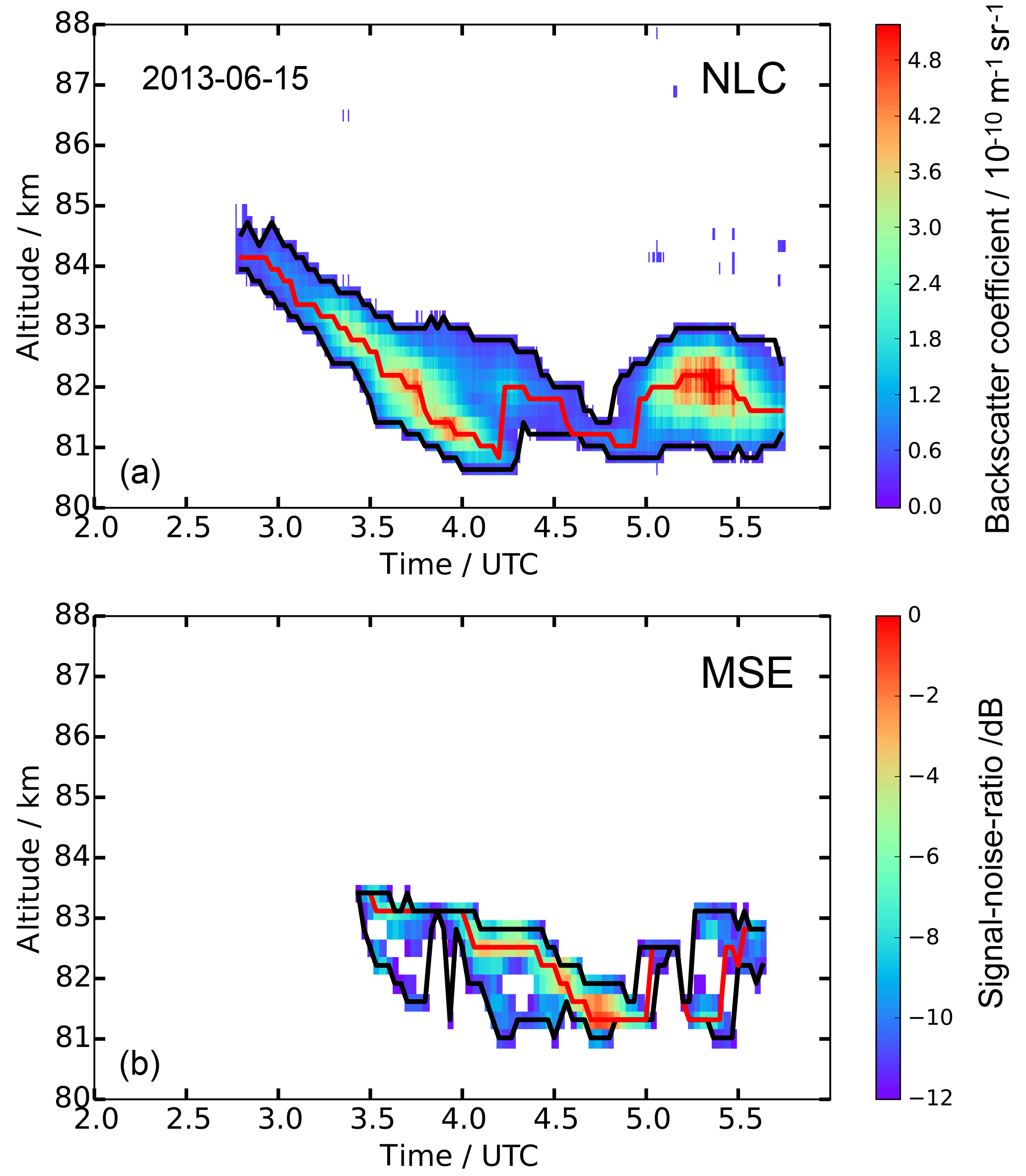
Figure 1Examples of detection of NLCs (a) and MSEs (b) using observations on 15 June 2013. The black lines show the upper and lower edges (zlow and zup), the red line the layer maxima (zmax). Edge detection is done on the temporal resolution of the radar (2 min). Edges are defined at β=0.3 (NLC) and the SNR is −12 dB (MSE).
2.2 MSE observations by the OSWIN VHF radar at Kühlungsborn
The monostatic OSWIN VHF radar (53.5 MHz) operated in an unattended and continuous measurement mode during the summer seasons. Until 2013 a phased-array antenna field consisting of 12×12 Yagi antennas was used. The beam could be tilted, but for the comparisons of MSEs and NLCs only the vertically directed beam with a beam width of 6∘ was selected. Two 16 bit complementary codes with 2 µs pulse elements were used. The repetition frequency was set to 1200 Hz. For reception, the antenna array was split in six subgroups with 24 antennas each, which were connected to six receivers. Data points were created by coherent integrations of 20 samples. Time series of 1024 data points are acquired within 34.1 s. Considering the time of further alternating measurements, the time resolution for MSE observations is 2 min. After 2013 the antenna array was refurbished. The new array is based on 133 Yagi antennas arranged in a hexagonal structure. The width of the vertically directed beam is about 6∘ again. Two 32 bit complementary codes with 2 µs pulse elements and 625 Hz repetition frequency are used. For reception, six subgroups of 21 antennas each are connected to six receivers. Time series of 1024 samples (inclusive of eight coherent integrations) result in a length of 26.2 s. In summary we assume fairly similar technical conditions regarding the radar measurements during the summer seasons. In both periods a height resolution of 300 m is maintained. The backscattered signals received by the six receivers are combined phase conform. Signal-to-noise ratios (SNRs) are estimated from the autocorrelation functions of the time series in each height channel. As we do not have an absolute calibration of the radar, we use the SNR as an approximation for the echo intensity. The lowest signal level used for MSE observations is chosen at a SNR of −12 dB. A typical example with identified edges is presented in Fig. 1b.
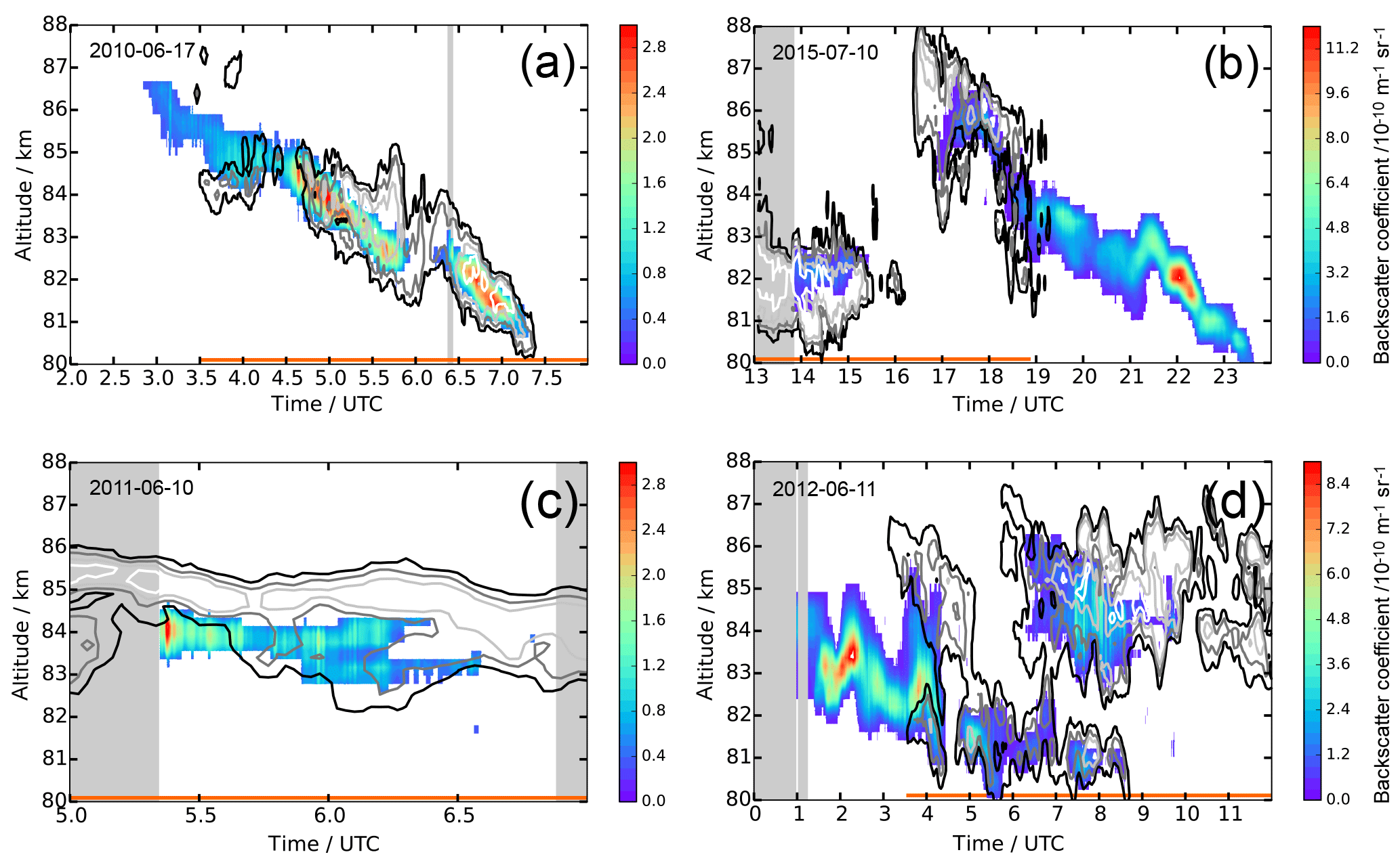
Figure 2Examples of observations of MSEs (contour lines at −12/−6/0/6 dB, if applicable) and NLCs (filled contours with scale on the right). The orange lines indicate periods with solar elevation >5∘. The gray shaded areas mark periods without lidar soundings due to the presence of clouds. (a) 17 June 2010: the MSE starts after sunrise into existing NLCs. (b) 10 July 2015: the MSE vanishes after sunset while the NLC continues. (c) 10 June 2011: when the lidar operation begins, the NLC is immediately detected, but does not extend as high as the MSE. (d) 11 June 2012: the MSE starts after sunrise when the NLC already existed and continues especially at higher altitudes when the NLC disappears.
2.3 Examples of simultaneous NLC–MSE observations
In the following we show different cases of simultaneous NLC–MSE observations to demonstrate the variability of the layers. Similar to previous studies, we often find very good agreement between NLCs and MSEs, while there are differences in other cases (Kaifler et al., 2011; Klekociuk et al., 2008; von Zahn and Bremer, 1999). Examples are given in Fig. 2. Figure 2a shows an event that was observed on 17 June 2010. While the NLC (filled contours) was first detected above the limit of β=0.3 at 02:45 UTC, the MSE (contour lines) was only observed after 03:30 UTC, when the solar elevation exceeded ∼5∘ and the ionization of the atmosphere was large enough to allow a radar backscatter signal. Then both phenomena follow the same vertical movement, presumably related to the cold phase of a gravity wave, with the MSE sometimes reaching to higher altitudes.
Also on 10 July 2015 (Fig. 2b) the NLC and the MSE showed a good agreement. The lidar was switched on at 13:50 UTC when the MSE already existed, and the NLC was observed from the beginning of the lidar sounding, but in a smaller altitude range. Between 15:30 and 16:50 UTC the NLC vanished, but the MSE showed only a short gap of 10 min and set in again at a much higher altitude about half an hour before the NLC occurred again. Then both layers agreed well until the MSE disappeared at ∼19:00 UTC at a solar elevation of ∼4∘. The NLC observation continued for another 5 h, until the layer descended below 80 km at 00:00 UTC.
On 10 June 2011 (Fig. 2c) the NLC was observed from the beginning of the lidar sounding at 05:21 UTC. Earlier, the ice particles were already detected by the radar as MSEs, but tropospheric clouds inhibited lidar operation. In contrast to the other cases, here the MSE extended above the NLC and was in fact strongest at altitudes above the NLC upper edge. Later on, the NLC ceased while the MSE continued.
A rare example of a double ice layer was observed on 11 June 2012 (Fig. 2d). The cloud was first confirmed by the lidar, showing that the NLC was very variable in altitude due to the presence of gravity waves. After ∼03:20 UTC the NLC layer thickness increased to ∼5 km (81–86 km). Just at the same time the radar echo started due to increasing solar elevation, i.e., increasing ionization. The MSE quickly grew into a double layer, with a gap around 83 km altitude, where the NLC was found to be brightest. The NLC and MSE around 82 km faded away at 04:23 UTC and set in again at 04:40/04:45 UTC (MSE/NLC). In the meantime, the only remaining ice signal was observed by the radar above 83 km. Past ∼05:00 UTC the upper MSE layer vanished, but reappeared shortly after. At ∼06:15 UTC the NLC also formed a (very rare) double layer until ∼08:30 UTC, when the lower layer of both the NLC and the MSE ceased. Despite being weak, the upper NLC layer remained observable until ∼10:00 UTC, while the MSE still continued in a broad range (83–87 km). The variable structure of the ice cloud with double layers indicates a highly dynamic behavior of the atmosphere with the presence of strong gravity waves. Nevertheless, a detailed examination of the dynamical structure is beyond the scope of this paper.
The examples shown above demonstrate the different relations of the NLC and MSE layer edges and the different degrees of accordance of the layers. This is in general agreement with observations at polar latitudes (Kaifler et al., 2011; Klekociuk et al., 2008). The examples indicate an often good concurrence of the lower edges but a worse agreement of the upper edges. If solar elevation (i.e., ionization) is sufficiently large, NLCs are often but not always accompanied by MSEs. The latter might be explained by the radar detection threshold or missing turbulence, but this cannot be checked here because a lack of appropriate measurements. Periods with MSEs but absent NLCs can be caused by mainly small ice particles, resulting in lidar signals below the NLC detection threshold. In the following we neglect profiles of NLCs without MSEs as well as MSEs without NLCs to be sure that for this study all requirements for the observation of small and large ice particles are fulfilled (see below).
2.4 The data set used for this study
Within this study we only focus on simultaneous NLC and MSE events (e.g., after 03:30 UTC in Fig. 2a, but excluding the little MSE gaps between 04:00 and 05:00 UTC), to compare the altitude ranges in which both phenomena are observed. Nighttime NLCs, for which ionization of the atmosphere is typically too small for MSE generation, are ignored as well as a few NLCs for which the radar was switched off for maintenance. Conversely, we do not count ice clouds (detected as MSEs) that are found too weak to be observed by lidar or that occurred when the lidar was switched off, e.g., during tropospheric cloud coverage. Overall, we use ∼67 h of NLCs with β>0.3 for this study, out of 188.5 h of NLCs in total (β>0, day and night) in the years 2010–2016. About 121 h of NLC detection cannot be used here because of either too weak NLCs (β<0.3, ∼20 %) or the absence of MSEs. MSEs get sparse at low solar elevation because of missing ionization (∼35 % of the time the solar elevation is below 5∘). Furthermore, either turbulence can be missing or the radar detection threshold can be too high. Nevertheless, this subset of NLCs is representative of the whole data set in terms of layer heights, as discussed in Sect. 5. The total usable lidar operation time within the seven summers (1 June to 4 August) is 3337 h. MSEs are observed by OSWIN for 960 out of 8600 h total sounding time. As mentioned above, only for 67 h do the MSE (SNR>12 dB) occur during lidar operation and simultaneously with NLCs of β>0.3. These data are distributed across 31 days with an average ice cloud duration of 2.2 h. For this study it is not relevant whether the ice observation is uninterrupted in time or not because the layer parameters are derived based on individual (but smoothed) profiles. Note that this study is representative of ice clouds containing sufficiently large particles to be detectable by lidar, but it is not representative of MSEs (ice clouds) in general.
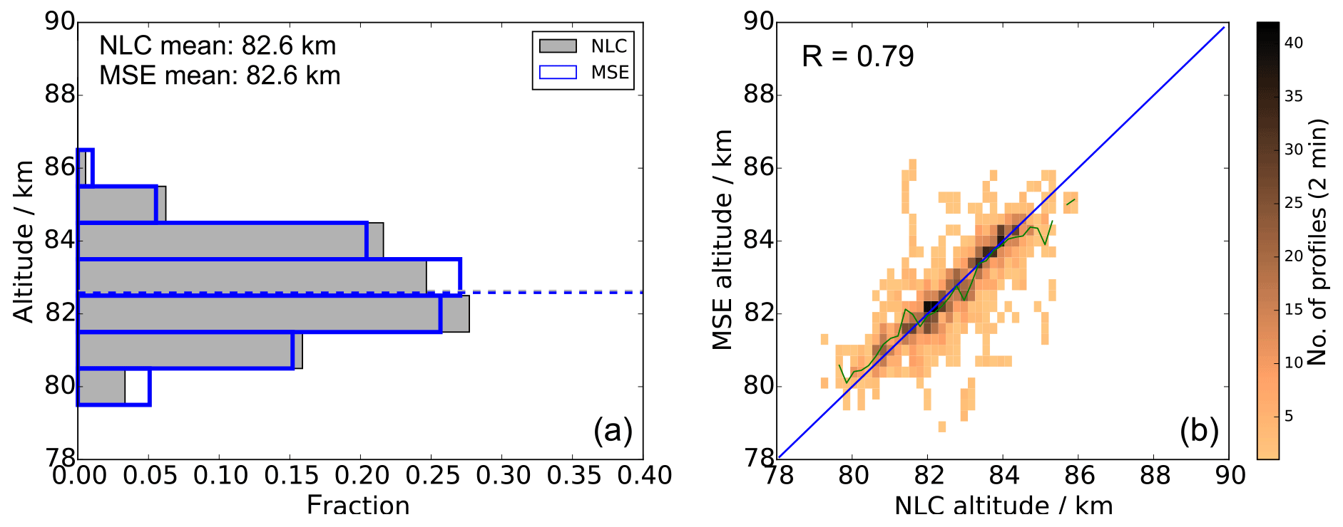
Figure 3Comparison of lower edges of NLCs and MSEs ( and ). (a) Histogram with NLC edges in grey (filled) and MSE edges in blue (open histogram). Mean values are indicated by the dashed lines. (b) Scatter plot of MSE and NLC edges. Only simultaneous soundings based on a 2 min temporal resolution are evaluated. The green line in (b) shows the average MSE lower edge altitude for each NLC edge bin, and the blue line indicates identical altitudes.
Based on the data set of simultaneous NLCs and MSEs (gridded to 2 min temporal resolution) we identify the lower edges ( and ), the altitudes of maximum brightness ( and ), and the upper edges ( and ) for each profile of both phenomena independently, as shown in Fig. 1. In the rare case of a double layer we take the lower edge of the lower layer and the upper edge of the upper layer together with the absolute maximum. Overall, we get 1931 profiles with their respective properties, even if the particular smoothing of lidar and radar data needs to be taken into account for interpretation. In Fig. 3a the altitude distributions of and are summarized in 1 km bins. The most striking feature is the similarity between the altitude distributions of NLC and MSE lower edges. In the evaluated data set, no cloud is observed below 80 km. The mean values of both and are found at ∼82.6 km (dashed lines). The figure only shows small differences between both distributions. In Fig. 3b the lower edges of all individual NLC and MSE profiles are compared. The plot confirms the similarity between both parameters. Most often the zlow agree within a single altitude bin, which also shows up in the correlation coefficient of R=0.79. The differences between and can be up to a few hundred meters, and there is no altitude dependence of the differences. Thus, very high ice clouds show the same similarity as low or typical layers. The mean difference between and is ∼40 m, with a standard deviation of 417 m. In a few cases the altitude difference can be up to 4–5 km. This can already be seen in Fig. 2d, e.g., in cases of MSE onset in the morning twilight when sometimes the MSE only agrees with the uppermost part (i.e., largest ionization) of the ice cloud. Part of the differences can also be explained by the different fields of view (FOV). The radar has a FOV of rad, while the lidar FOV is only of this (62 µrad). This may lead to some differences, at least in cases of very structured ice clouds, because any feature in the ice cloud needs some time for drifting through the radar FOV, e.g., ∼3.5 min at 20 m s−1 wind speed. Rarely, the different size dependencies of lidar and radar signals can lead to MSEs even a few kilometers below the NLCs. On average, these effects only have a small influence on the general distribution.
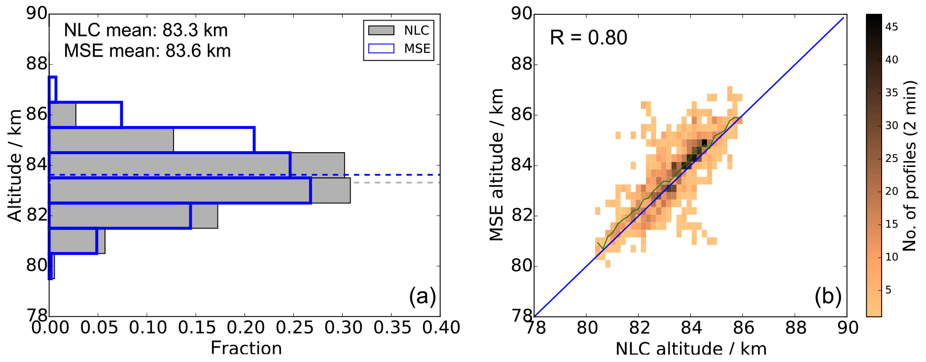
The altitude distribution of the ice layer maxima (backscatter coefficient for NLCs and signal-to-noise ratio for MSEs) is shown in Fig. 4. The mean of is observed at 83.3 km (grey dashed line in panel a), while the mean of is slightly higher at 83.6 km (blue dashed line in panel a). No NLC maximum is observed above 86 km, but a few MSE maxima are observed. This is also resembled in the scatter plot (Fig. 4b). Similar to the lower edges, there is no pronounced altitude dependence of the differences between and (green line). The correlation coefficient is R=0.80. While again the individual and sometimes differ by a few kilometers, the mean value of the differences is only ∼300 m, with a standard deviation of 375 m.
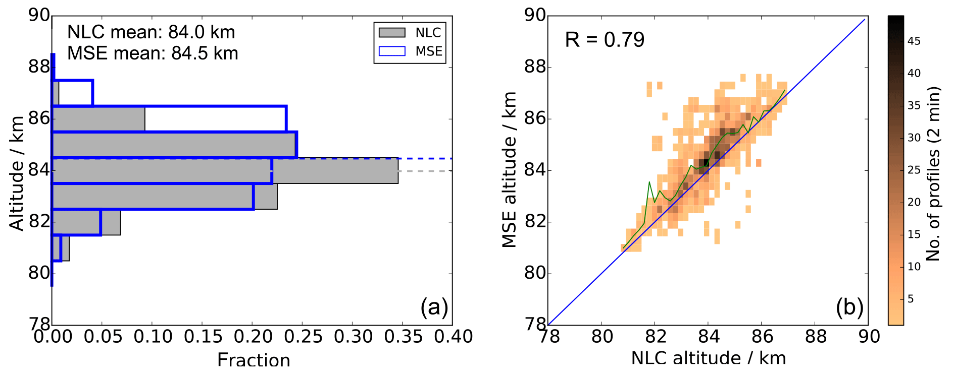
The largest differences between NLCs and MSEs are expected at the upper edges of the layer (Kaifler et al., 2011). This is due to the fact that the nucleation typically starts close to the mesopause, where water vapor saturation is largest. These small particles can already be detected by radars (signal strength proportional to r2, if turbulence and ionization allow). If the supersaturated region extends further down, the particles start to sediment and grow, and become finally visible for lidars (signal strength proportional to r5…r6). Indeed, we find the mean about 500 m above the mean for all simultaneous observations (Fig. 5), i.e., at 84.5 and 84.0 km, respectively. The scatter plot shows that the height difference is largely independent of altitude. Only for the very high (>85 km) and very low (<82 km) layers do the differences seem to vanish, but the number of such events is small. The smaller height difference can be explained by the typically smaller width of the ice clouds at these altitudes (not shown). In contrast to the layer maxima and lower edges, differences of a few kilometers are mainly found, with the MSE top being much higher than the NLC top. Thus, the distribution of differences is not symmetric, but has a tail towards higher MSEs as typically expected. Note that the correlation of and is still high (R=0.79).
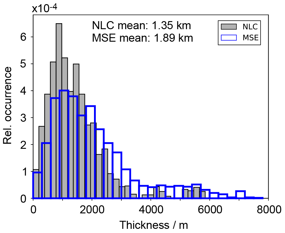
Figure 6Histogram of layer thicknesses, calculated as for NLCs (grey, filled) and for MSE (blue, open). The relative occurrence (O) is normalized such that all bins times the bin width (Δ) sum to 1; i.e., . Bin widths are 195 m for NLCs and 300 m for MSEs.

Figure 7Temperature (a) and meridional wind (b) above Kühlungsborn during 26 and 27 June 2011. The MSE data are embedded in both panels for illustration as open grey contours and the NLC data in colored filled contours. Cloud 1: 02:30–05:15 UTC, Cloud 2: 05:30–08:40 UTC.
From the upper and lower edges, the NLC and MSE layer thicknesses can easily be calculated. The results are shown in the histograms in Fig. 6. Typically, the NLC thickness () is below 2 km, with a mean value of 1.35 km. The MSEs are typically slightly thicker, having a mean layer thickness of 1.89 km. These numbers are already expected from the difference of mean upper and lower edges. Furthermore, the histogram shows a larger quantity of thick MSEs, with thicknesses of more than 4 km. That means that in a few cases the MSE width is much larger than the NLC width, but the average layer thicknesses differ by only ∼500 m.
There is general agreement that ice clouds are limited to regions with temperatures below the frost point temperature. For our location we have already shown that NLCs only occur in the cold phases of gravity and planetary waves, while mean temperatures are above the frost point in the whole mesopause region (Gerding et al., 2007, 2013a). Additionally, we demonstrated that southward-directed winds are necessary for the occurrence of NLCs at our site (Gerding et al., 2007, 2013b). Here we want to check whether the ambient wind and temperature conditions are responsible for the altitude of the layer edges, i.e., the thickness of the NLCs and MSEs. We therefore evaluated the temperatures and winds, especially above the layers.
Temperature soundings above MSEs require a metal resonance lidar (for the altitude coverage) and daylight capabilities (for observation during MSEs). The potassium resonance lidar at Kühlungsborn was in operation until the end of 2012; i.e., it covered part of the examined time period. Figure 7a shows an example of the temperature structure above two ice layers in the early morning of 27 June 2011. The first layer (“Cloud 1”) arose at ∼02:30 UTC in the lidar (NLC, colored layer) and did not extend above 83.5 km. The MSE (grey contour lines) appeared first at 03:30 UTC at 84.3 km, when ionization was sufficient (solar elevation 4.7∘). Above Cloud 1 the potassium resonance lidar observed temperatures of more than 150 K, i.e., higher than the expected frost point temperature for these altitudes. In other words, the temperature structure inhibits an expansion of the layer to higher altitudes. Later, Cloud 1 descended and vanished at 05:15 UTC. Another ice layer (“Cloud 2”) appeared at ∼05:30 UTC around 86 km. This coincides with a strong temperature decrease below ∼140 K in the same altitude range. We point out that Cloud 2 was observed by radar only (MSE), but did not contain particles large enough to be observed by lidar (NLC). Lidar observations stopped due to tropospheric clouds at ∼08:00 UTC. Note the integration time of the temperature data of 2 h, shortened to 1 h at the beginning and end of the sounding.
Figure 7b shows the meridional wind observed by the nearby meteor radar (120 km northeast of Kühlungsborn). The warm region above Cloud 1 is accompanied by a northward wind, while the wind in the altitude of the layer is southward, as expected from previous observations. At the time and altitude of (higher) Cloud 2 the wind direction changed to a weak southward wind. Overall, this typical case shows a large likelihood for advection of Cloud 1 that appeared as both an MSE and an NLC because local ice formation is inhibited by the high temperatures above 85 km. Note that before 02:00 UTC low temperatures of ∼140 K were observed above 85 km, but at this time no ice cloud was observed. The second case (Cloud 2) has the potential for local formation above 85 km, but this layer is confined to higher altitudes and does not contain larger ice particles (NLC). Both clouds are confined to southward winds.
We have analyzed the temperature and wind data set above the NLCs and MSEs for all available coincident measurements. Due to frequent hazy sky conditions and therefore a large solar background at near-infrared wavelengths, the temperature data set of the potassium lidar is smaller than the NLC data set of the RMR lidar. For the period between 2010 and 2012, only seven events can be evaluated, with some of the data sets showing a gap of up to 2 km between the NLCs and MSEs and the temperature data. The temperature structure above the ice clouds varies between the events. Partly, we find an immediate temperature increase above (five cases), inhibiting ice existence in these heights. In the other two cases, the supersaturated region extends for some kilometers above the observed ice cloud and includes the height region expected for nucleation (87–90 km; e.g., Kiliani et al., 2013). In this case, ice particles may still exist in the supersaturated region, even if not detected by the OSWIN radar. Low temperatures typically only persist for a few hours at our site (Gerding et al., 2007). In this time, ice particles only grow to a few nanometers' radius (Rapp and Thomas, 2006), and continuous turbulence is needed to create radar echoes, in contrast to intermittent turbulence being sufficient in combination with larger ice particles (Rapp and Lübken, 2004). Additional ionization is needed in both cases. Unfortunately, there is no information about ambient turbulence available and the question about ice existence cannot be finally answered.
The wind structure above the NLCs and MSEs is also not uniform in all events. Overall, 23 events between 2010 and 2016 have been evaluated. During most of the events (nine cases) the wind above the ice layer was southward (as in the ice layer). Seven cases show northward winds above the cloud. In three cases the wind direction was changing, while four cases only showed weak winds (less than ±10 m s−1).
Studies on the layer properties of NLCs and MSEs at midlatitudes are rare because there is only a small occurrence frequency of 5 %–10 % for MSEs and NLCs (Gerding et al., 2013a; Thomas et al., 1996; Zecha et al., 2003). Therefore, analyses of average layer parameters need multiyear observations to yield a representative database. The only statistical NLC study at midlatitudes has been done at our site at Kühlungsborn based on the nighttime observations of the previous RMR lidar (Gerding et al., 2013a). The results are in good agreement with the data presented here. They report a mean centroid height of 82.7 km, which compares very well with the mean centroid height of 82.6 km and mean peak height of 82.8 km of all NLCs (daytime and nighttime) in the 2010–2016 period used here. Selecting only days that also show MSEs, the mean NLC peak height is slightly higher (83.0 km), but within the geophysical variability. The remaining difference to the mean of 83.3 km mentioned in Fig. 4 can be explained by the further selection of profiles really showing simultaneous MSEs. Especially some very low NLC profiles (below 80 km) are excluded here because of missing MSEs, which is potentially caused by the reduced electron density. Furthermore, the faintest NLC profiles with β<0.3, e.g., in the beginning and end of events, are also excluded in Fig. 4. Therefore the apparent difference in NLC layer heights compared to previous studies can be explained by geophysical variability and treatment of the NLC data. But this does not hamper the representativeness of this study for all NLCs.
For MSEs there is an earlier study by Zecha et al. (2003) using radar data from Kühlungsborn. They report the occurrence rate of MSEs at each particular height bin which is different from the histogram of peak altitudes that we present here. Even more important, we limit the MSE data set to events with simultaneous NLCs because we want to focus on optically visible ice clouds. By this we suppress weak and high (typically >86 km) layers of MSEs that are often not accompanied by NLCs. We note that we skip the majority of MSEs by this selection. Therefore, the results presented here are not representative of all MSEs.
As explained above, there are only very few studies for high-latitude, simultaneous NLCs and PMSEs. Kaifler et al. (2011) evaluated a large data set of NLCs and PMSEs from ALOMAR (69∘ N, 16∘ E). Simultaneous events are summarized in their categories III, IV, and V. In their Table 3 they also report quasi-identical lower edges of NLCs and PMSEs, even if the zlow at higher latitudes are observed 0.5 km below the midlatitude values. The identity of NLC and MSE lower edges is to some extent induced by the data selection criteria. Kaifler et al. (2011) only used NLCs with a peak brightness of β>4, shifting the lower edge a few hundred meters down compared to all NLCs (their Fig. 5). We find a similar effect in our data set (not shown). This explains, together with the fact that NLCs are thinner at midlatitudes, the altitude difference of NLC lower edges between high latitudes and midlatitudes.
Regarding the upper edges ( and ), Kaifler et al. (2011) report a mean difference of ∼3.3 km, i.e., much larger than the difference of 0.5 km that we observe at midlatitudes. Klekociuk et al. (2008) examined one season of simultaneous observations of NLCs and PMSEs at 69∘ S at Davis Station (Antarctica). Occurrence rates of both phenomena are much smaller compared to the Northern Hemisphere. The authors do not provide numbers for the upper and lower edges of the layers, but from their Fig. 1 one can expect a difference of the upper edges similar to the numbers given by Kaifler et al. (2011). We therefore examined whether the small difference presented here is an arbitrary result of our limited data set. We chose different sub-data sets containing about half of the profiles, either using a random process or by selecting only the first or second half of the data. The small difference of upper edges persisted throughout all selection runs, varying between 0.2 and 0.7 km.
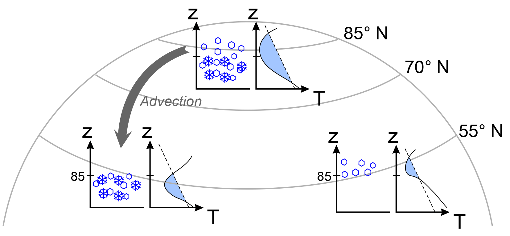
Figure 8Schematic of the latitudinal differences for ice cloud formation. The x–y plots represent the ice particle distribution with height (left) and the corresponding temperature profile (right). Small particles only visible for the radar are marked by light blue hexagons, larger particles by blue snowflakes. The light blue part of the temperature profile shows the region of supersaturation (dashed: frost point temperature). The altitude of 85 km is marked, forming a typical upper limit of NLCs.
The reason for the large height difference between and at high latitudes is the typically much larger thickness of the PMSE layer (cf. our Fig. 6, and Table 3 in Kaifler et al. (2011)). In agreement with these observations, using a 3-D trajectory model, Kiliani et al. (2013) demonstrated the formation of ice particles at the high-latitude mesopause, and subsequent descent and growth. At high latitudes often a layer of small particles (only visible by radar) exists above the larger ice particles that can also be detected by lidar. This situation is in qualitative agreement with Odin/OSIRIS observations (Hultgren and Gumbel, 2014) and sketched in the upper part of Fig. 8. The small difference between upper layer edges in our observations suggests that the layer of small particles is missing at midlatitudes. In this case, the larger, optically visible ice particles cannot be formed locally, but typically have to be advected (see lower left part of Fig. 8). Kiliani et al. (2013) found in their simulations that the last ∼6 h before observation were most relevant for particle growth. In this period, the ice particles typically travel 150–500 km southward. Before, the ice particles remained small (<20 nm) for more than 60 h. In agreement with this, NLCs above Kühlungsborn are generally observed during southward wind conditions (Gerding et al., 2007, 2013a, b), and also in the Southern Hemisphere, NLCs are typically limited to equatorward winds, even at high latitudes (69∘ S) (Klekociuk et al., 2008; Morris et al., 2007). In contrast, Stevens et al. (2017) found a dominating dependence of NLCs on local temperatures, even at midlatitudes, using NOGAPS-ALPHA assimilated model data. The authors explicitly neglected transport effects by using a 0-D NLC model, making a direct comparison with our findings difficult. Similarly, Herron et al. (2007) and Hultgren et al. (2011) found local effects dominating the formation of NLCs for their midlatitude observations.
Furthermore, we cannot exclude longitudinal differences for the formation of ice clouds. According to SOFIE observations our site is at the longitude of minimal NLC occurrence rates (Hervig et al., 2016), suggesting different cloud formation mechanisms compared to other longitudes. It has been shown before for our site that temperatures below the frost point as well as southward winds are necessary but not sufficient criteria for NLC observations (Gerding et al., 2007). Supersaturated regions upstream of Kühlungsborn are needed to foster the nucleation process and to allow for the particles to grow to sufficient sizes (Fig. 8, lower left). About one-third of the events examined here show southward winds also above the layer. The fact that these air parcels do not contain ice particles again confirms that southward winds are necessary but not sufficient for ice existence above our site. On the other hand, in another third of our events we found northward winds directly above the cloud, i.e., advecting air from (presumably) warmer regions. We would like to note that the OSWIN radar often detects MSEs in thin layers above 85 km altitude (Zecha et al., 2003). We cannot exclude that these MSEs are formed by ice particles nucleated close by. But these particles typically do not reside long enough at our site to grow to sizes that allow optical detection, or the supersaturated height range is too thin to allow effective growth during sedimentation. This is sketched in the lower right part of Fig. 8.
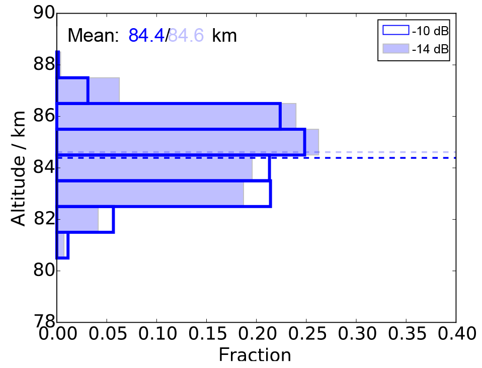
Figure 9Same as Fig. 5, but with different MSE thresholds. Blue, open bars show the MSE threshold SNR of −10 dB; light blue filled bars show the MSE threshold SNR of −14 dB.
In contrast to the upper edges, the lower edges of NLCs and PMSEs at 69∘ N typically agree quite well (Kaifler et al., 2011), similar to our observations. This is in fact expected due to the fast sublimation of the ice particles with typically rising temperatures at the lower edge of the layer. Of course, the instrument's sensitivity needs to be taken into account for the comparison of layer edges. For the lidar observations described here we set the threshold to β=0.3, which is slightly smaller than the threshold used in Gerding et al. (2013b) for the same lidar (β=0.5). We confirmed by manual inspection that the edges of the individual NLCs are correctly identified and not affected by background noise. We processed the radar data in units of SNR. The threshold is set to −12 dB to be above the typical noise limit of the radar. We tested the influence of this threshold by setting it to larger and smaller numbers. Figure 9 shows the same histogram as Fig. 5, but for thresholds of −10 and −14 dB. As expected, the mean rises to 84.6 km if weaker MSEs are also included. Limiting the data to dB, we found the mean at 84.4 km. In other words, the mean shift between both test scenarios is only 200 m, i.e., less than one altitude bin of the radar (300 m). Changing the NLC threshold has similar results. Here the gradients at the layer edges are also very large (see, e.g., Fig. 2) and a change of the threshold to, e.g., β=0.5 would only result in minor changes of the histograms. Therefore, there are only minor effects of the thresholds on layer edges, while the layer maximum is not affected at all. In any case, the changes due to threshold adaptions are much smaller than the difference to observations at higher latitudes.
In this study we compared NLC and MSE altitudes from simultaneous observations at our midlatitude site, Kühlungsborn (54∘ N, 12∘ E). There is general agreement that both phenomena represent ice clouds, with the visible echoes (NLCs) being formed by ice particles of typically some tens of nanometers' diameter. The radar echoes (MSEs) can also be formed by smaller particles, but require a sufficient density of free electrons as well as structures in the plasma. We have presented examples of NLC-only and MSE-only periods as well as for simultaneous layers with at least partial overlap in the covered altitude region. For the average layer parameters we only concentrated on simultaneous detections; i.e., we discarded nighttime NLCs because of electron densities that are typically too small to form MSEs. Furthermore we discarded all those high and weak MSEs that are not accompanied by NLCs. Overall, we obtained ∼67 h of NLC and MSE data within the summers 2010–2016.
On average, the lower edges of NLCs and MSEs are identical, which is in agreement with the general understanding of quickly sublimating ice particles at the bottom of the layer. The average values for the layer peaks and for the upper edges differ by 0.3 and 0.5 km, respectively, with the MSEs being slightly above the NLC. This comparatively small difference is in contrast to the observations at polar latitudes, where the PMSEs often extend several kilometers above the NLC. We found that the ice cloud itself is much thinner compared to polar latitudes (under the assumption that the MSE layer thickness at midlatitudes is not limited by smaller electron density or missing turbulence). Clouds that already exist long enough to form large particles (NLCs) only show a thin layer of small particles (invisible for the lidar but visible as MSEs) above the NLC at our site. Or they show no particles at all above the NLC; i.e., the upper edges of the NLC and the MSE coincide. Using simultaneous resonance lidar temperature soundings, we typically found the atmosphere above the layer to be too warm for ice existence, limiting the potential extent of the cloud. Meridional winds above the NLCs do not show a preferential direction for the examined events. Altogether, these observations give evidence that local formation of MSEs is possible, but these ice particles do not stay long enough to grow to optically visible sizes. All layers that are observed as NLCs are already formed and then advected to our site by the meridional wind. During advection and descent, the smaller particles grow to sizes of some tens of nanometers. Because of this, they become detectable by lidar. This formation process must be taken into account if, e.g., midlatitude NLC observations are used to study trends or climate change in the mesopause region.
The data presented in this paper are available at ftp://ftp.iap-kborn.de/data-in-publications/GerdingACP2018/, last access: 19 October 2018.
MG and MZ analyzed the NLC and the MSE data, respectively. Analysis and interpretation of the combined data set were done by JZ and MG. KB coordinated the lidar measurements and took part in the discussion of the manuscript. JH and GS provided the potassium lidar temperature data and the meteor radar wind data, respectively. FJL contributed to the discussion of the results and the manuscript. Finally, MG prepared the paper with feedback from all authors.
The authors declare that they have no conflict of interest.
This article is part of the special issue “Layered phenomena in the mesopause region (ACP/AMT inter-journal SI)”. It is a result of the LPMR workshop 2017 (LPMR-2017), Kühlungsborn, Germany, 18–22 September 2017.
We thank our colleagues Torsten Köpnick, Reik Ostermann, Michael Priester,
and Jörg Trautner for their support in lidar and radar operation and
maintenance. We acknowledge the contributions of numerous students helping
with continuous lidar soundings. Part of this work was supported by the
Deutsche Forschungsgemeinschaft (DFG) under grant GE 1625/2-1. We thank the
reviewers for their valuable comments that improved the manuscript.
The publication of this article was funded by the
Open Access Fund of the Leibniz Association.
Edited by: Martin Dameris
Reviewed by: two anonymous referees
Alpers, M., Eixmann, R., Fricke-Begemann, C., Gerding, M., and Höffner, J.: Temperature lidar measurements from 1 to 105 km altitude using resonance, Rayleigh, and Rotational Raman scattering, Atmos. Chem. Phys., 4, 793–800, https://doi.org/10.5194/acp-4-793-2004, 2004. a
Baumgarten, K., Gerding, M., Baumgarten, G., and Lübken, F.-J.: Temporal variability of tidal and gravity waves during a record long 10-day continuous lidar sounding, Atmos. Chem. Phys., 18, 371–384, https://doi.org/10.5194/acp-18-371-2018, 2018. a
Chilson, P. B., Czechowsky, P., Klostermeyer, J., Rüster, R., and Schmidt, G.: An investigation of measured temperature profiles and VHF mesosphere summer echoes at midlatitudes, J. Geophys. Res., 102, 23819–23828, https://doi.org/10.1029/97JD01572, 1997. a
Chu, X., Gardner, C. S., and Roble, R. G.: Lidar studies of interannual, seasonal, and diurnal variations of polar mesospheric clouds at the South Pole, J. Geophys. Res., 108, 8447, https://doi.org/10.1029/2002JD002524, 2003. a
Collins, R., Taylor, M., Nielsen, K., Mizutani, K., Murayama, Y., Sakanoi, K., and DeLand, M.: Noctilucent cloud in the western Arctic in 2005: Simultaneous lidar and camera observations and analysis, J. Atmos. Sol.-Terr. Phy., 71, 446–452, https://doi.org/10.1016/j.jastp.2008.09.044, 2009. a
DeLand, M. T., Shettle, E. P., Thomas, G. E., and Olivero, J. J.: Solar backscattered ultraviolett (SBUV) observations of polar mesospheric clouds (PMCs) over two solar cycles, J. Geophys. Res., 108, 8445, https://doi.org/10.1029/2002JD002398, 2003. a
Fiedler, J., Baumgarten, G., Berger, U., and Lübken, F.-J.: Long-Term Variations of Noctilucent Clouds at ALOMAR, J. Atmos. Sol.-Terr. Phy., 162, 79–89, https://doi.org/10.1016/j.jastp.2016.08.006, 2017. a
Gerding, M., Höffner, J., Rauthe, M., Singer, W., Zecha, M., and Lübken, F.-J.: Simultaneous observation of NLC, MSE and temperature at a midlatitude station (54∘ N), J. Geophys. Res., 112, D12111, https://doi.org/10.1029/2006JD008135, 2007. a, b, c, d, e
Gerding, M., Höffner, J., Hoffmann, P., Kopp, M., and Lübken, F.-J.: Noctilucent Cloud variability and mean parameters from 15 years of lidar observations at a mid-latitude site (54∘ N, 12∘ E), J. Geophys. Res., 118, 317–328, https://doi.org/10.1029/2012JD018319, 2013a. a, b, c, d, e, f
Gerding, M., Kopp, M., Hoffmann, P., Höffner, J., and Lübken, F.-J.: Diurnal variations of midlatitude NLC parameters observed by daylight-capable lidar and their relation to ambient parameters, Geophys. Res. Lett., 40, 6390–6394, https://doi.org/10.1002/2013GL057955, 2013b. a, b, c, d
Gerding, M., Kopp, M., Höffner, J., Baumgarten, K., and Lübken, F.-J.: Mesospheric temperature soundings with the new, daylight-capable IAP RMR lidar, Atmos. Meas. Tech., 9, 3707–3715, https://doi.org/10.5194/amt-9-3707-2016, 2016. a
Herron, J. P., Wickwar, V. B., Espy, P. J., and Meriwether, J. W.: Observations of a noctilucent cloud above Logan, Utah (41.7∘ N, 111.8∘ W) in 1995, J. Geophys. Res., 112, D19203, https://doi.org/10.1029/2006JD007158, 2007. a, b
Hervig, M. E., Gerding, M., Stevens, M. H., Stockwell, R., Bailey, S. M., Russell III, J. M., and Stober, G.: Mid-latitude mesospheric clouds and their environment from SOFIE, J. Atmos. Sol.-Terr. Phy., 149, 1–14, https://doi.org/10.1016/j.jastp.2016.09.004, 2016. a
Hultgren, K. and Gumbel, J.: Tomographic and spectral views on the lifecycle of polar mesospheric clouds from Odin/OSIRIS, J. Geophys. Res., 119, 14129–14143, https://doi.org/10.1002/2014JD022435, 2014. a
Hultgren, K., Körnich, H., Gumbel, J., Gerding, M., Hoffmann, P., Lossow, S., and Megner, L.: What caused the exceptional mid-latitudinal noctilucent cloud event in July 2009, J. Atmos. Sol.-Terr. Phy., 73, 2125–2131, 2011. a, b
Kaifler, N., Baumgarten, G., Fiedler, J., Latteck, R., Lübken, F.-J., and Rapp, M.: Coincident measurements of PMSE and NLC above ALOMAR (69∘ N, 16∘ E) by radar and lidar from 1999–2008, Atmos. Chem. Phys., 11, 1355–1366, https://doi.org/10.5194/acp-11-1355-2011, 2011. a, b, c, d, e, f, g, h, i, j
Kiliani, J., Baumgarten, G., Lübken, F.-J., Berger, U., and Hoffmann, P.: Temporal and spatial characteristics of the formation of strong noctilucent clouds, J. Atmos. Sol.-Terr. Phy., 104, 151–166, https://doi.org/10.1016/j.jastp.2013.01.005, 2013. a, b, c
Klekociuk, A. R., Morris, R. J., and Innis, J. L.: First Southern Hemisphere common-volume measurements of PMC and PMSE, Geophys. Res. Lett., 35, L24804, https://doi.org/10.1029/2008GL035988, 2008. a, b, c, d, e
Kopp, M., Gerding, M., Höffner, J., and Lübken, F.-J.: Tidal signatures in temperatures derived from daylight lidar soundings above Kühlungsborn (54∘ N, 12∘ E), J. Atmos. Sol.-Terr. Phy., 127, 37–50, https://doi.org/10.1016/j.jastp.2014.09.002, 2015. a
Kubo, K., Sugiyama, T., Nakamura, T., and Fukao, S.: Seasonal and interannual variability of mesospheric echoes observed with the middle and upper atmosphere radar during 1986–1995, Geophys. Res. Lett., 24, 1211–1214, https://doi.org/10.1029/97GL01063, 1997. a
Latteck, R. and Bremer, J.: Long-term variations of polar mesospheric summer echoes observed at Andoya (69∘ N), J. Atmos. Sol.-Terr. Phy., 163, 31–37, https://doi.org/10.1016/j.jastp.2017.07.005, 2017. a, b, c
Latteck, R., Singer, W., and Höffner, J.: Mesosphere summer echoes as observed by VHF radar at Kühlungsborn (54∘N), Geophys. Res. Lett., 26, 1533–1536, https://doi.org/10.1029/1999GL900225, 1999. a
Leslie, R. C.: Sky glows, Nature, 32, 245, 1885. a
Li, Q., Rapp, M., Röttger, J., Latteck, R., Zecha, M., Strelnikova, I., Baumgarten, G., Hervig, M., Hall, C., and Tsutsumi, M.: Microphysical parameters of mesospheric ice clouds derived from calibrated observations of polar mesosphere summer echoes at Bragg wavelengths of 2.8 m and 30 cm, J. Geophys. Res., 115, D00I13, https://doi.org/10.1029/2009JD012271, 2010. a
Morris, R. J., Murphy, D. J., Klekociuk, A. R., and Holdsworth, D. A.: First complete season of PMSE observations above Davis, Antarctica, and their relation to winds and temperatures, Geophys. Res. Lett., 34, L05805, https://doi.org/10.1029/2006GL028641, 2007. a, b, c, d
Muraoka, Y., Sugiyama, T., Sato, T., Tsuda, T., and Fukao, S.: Interpretation of layered structure in mesospheric VHF echoes induced by an inertia gravity wave, Radio Sci., 24, 393–406, https://doi.org/10.1029/RS024i003p00393, 1989. a
Nielsen, K., Nedoluha, G. E., Chandran, A., Chang, L. C., Barker-Tvedtnes, J., Taylor, M. J., Mitchell, N. J., Lambert, A., Schwartz, M. J., and Russell III, J. M.: On the origin of mid-latitude mesospheric clouds: The July 2009 cloud outbreak, J. Atmos. Sol.-Terr. Phy., 73, 2118–2124, https://doi.org/10.1016/j.jastp.2010.10.015, 2011. a
Nussbaumer, V., Fricke, K. H., Langer, M., Singer, W., and von Zahn, U.: First simultaneous and common volume observations of noctilucent clouds and polar mesosphere summer echoes by lidar and radar, J. Geophys. Res., 101, 19161–19167, 1996. a
Ogawa, T., Kawamura, S., and Murayama, Y.: Mesosphere summer echoes observed with VHF and MF radars at Wakkanai, Japan (45.4∘ N), J. Atmos. Sol.-Terr. Phy., 73, 2132 – 2141, https://doi.org/10.1016/j.jastp.2010.12.016, 2011. a
Rapp, M. and Lübken, F.-J.: Polar mesosphere summer echoes (PMSE): Review of observations and current understanding, Atmos. Chem. Phys., 4, 2601–2633, https://doi.org/10.5194/acp-4-2601-2004, 2004. a, b, c
Rapp, M. and Thomas, G. E.: Modeling the microphysics of mesospheric ice particles: Assessment of current capabilities and basic sensitivities, J. Atmos. Sol.-Terr. Phy., 68, 715–744, https://doi.org/10.1016/j.jastp.2005.10.015, 2006. a
Russell, J. M., Rong, P., Hervig, M. E., Siskind, D. E., Stevens, M. H., Bailey, S. M., and Gumbel, J.: Analysis of northern midlatitude noctilucent cloud occurrences using satellite data and modeling, J. Geophys. Res., 119, 3238–3250, https://doi.org/10.1002/2013JD021017, 2014. a, b
Stevens, M. H., Lieberman, R. S., Siskind, D. E., McCormack, J. P., Hervig, M. E., and Englert, C. R.: Periodicities of polar mesospheric clouds inferred from a meteorological analysis and forecast system, J. Geophys. Res., 122, 4508–4527, https://doi.org/10.1002/2016JD025349, 2017. a, b
Stober, G., Jacobi, C., Matthias, V., Hoffmann, P., and Gerding, M.: Neutral air density variations during strong planetary wave activity in the mesopause region derived from meteor radar observations, J. Atmos. Sol.-Terr. Phy., 74, 55–63, https://doi.org/10.1016/j.jastp.2011.10.007, 2012. a
Stober, G., Matthias, V., Jacobi, C., Wilhelm, S., Höffner, J., and Chau, J. L.: Exceptionally strong summer-like zonal wind reversal in the upper mesosphere during winter 2015/16, Ann. Geophys., 35, 711–720, https://doi.org/10.5194/angeo-35-711-2017, 2017. a
Thomas, G. E.: Are noctilucent clouds harbingers of global change in the middle atmosphere?, Adv. Space Res., 32, 1737–1746, https://doi.org/10.1016/S0273-1177(03)90470-4, 2003. a
Thomas, L., Marsh, A. K. P., Wareing, D. P., and Hassan, M. A.: Lidar observations of ice crystals associated with noctilucent clouds at middle latitudes, Geophys. Res. Lett., 21, 385–388, 1994. a
Thomas, L., Marsh, A. K. P., Wareing, D. P., Astin, I., and Chandra, H.: VHF echoes from the midlatitude mesosphere and the thermal structure observed by lidar, J. Geophys. Res.-Atmos., 101, 12867–12877, https://doi.org/10.1029/96JD00218, 1996. a, b
von Zahn, U. and Bremer, J.: Simultaneous and common-volume observations of noctilucent clouds and polar mesosphere summer echoes, Geophys. Res. Lett., 26, 1521–1524, https://doi.org/10.1029/1999GL900206, 1999. a, b
von Zahn, U. and Höffner, J.: Mesopause temperature profiling by potassium lidar, Geophys. Res. Lett., 23, 141–144, https://doi.org/10.1029/95GL03688, 1996. a
Wickwar, V. B., Taylor, M. J., Herron, J. P., and Martineau, B. A.: Visual and lidar observations of noctilucent clouds above Logan, Utah, at 41.7∘ N, J. Geophys. Res., 107, 1–7, https://doi.org/10.1029/2001JD001180, 2002. a
Zecha, M., Bremer, J., Latteck, R., Singer, W., and Hoffmann, P.: Properties of midlatitude mesosphere summer echoes after three seasons of VHF radar observations at 54∘ N, J. Geophys. Res., 108, 8439, https://doi.org/10.1029/2002JD002442, 2003. a, b, c, d, e
Zeller, O., Hoffmann, P., Bremer, J., and Singer, W.: Mesosphere summer echoes, temperature, and meridional wind variations at mid- and polar latitudes, J. Atmos. Sol.-Terr. Phy., 71, 931 – 942, https://doi.org/10.1016/j.jastp.2009.03.013, 2009. a
- Abstract
- Introduction
- Methodology and single-layer comparison
- Comparison of NLC and MSE layer properties
- Comparison of NLCs and MSEs with local wind and temperature structure
- Discussion
- Summary and conclusions
- Data availability
- Author contributions
- Competing interests
- Special issue statement
- Acknowledgements
- References