the Creative Commons Attribution 4.0 License.
the Creative Commons Attribution 4.0 License.
 | 29 Oct 2018
A deep stratosphere-to-troposphere ozone transport event over Europe simulated in CAMS global and regional forecast systems: analysis and evaluation
Eleni Katragkou
Prodromos Zanis
Ioannis Pytharoulis
Dimitris Melas
Johannes Flemming
Antje Inness
Hannah Clark
Matthieu Plu
Henk Eskes
Stratosphere-to-troposphere transport (STT) is an important natural source of tropospheric ozone, which can occasionally influence ground-level ozone concentrations relevant for air quality. Here, we analyse and evaluate the Copernicus Atmosphere Monitoring Service (CAMS) global and regional forecast systems during a deep STT event over Europe for the time period from 4 to 9 January 2017. The predominant synoptic condition is described by a deep upper level trough over eastern and central Europe, favouring the formation of tropopause folding events along the jet stream axis and therefore the intrusion of stratospheric ozone into the troposphere. Both global and regional CAMS forecast products reproduce the “hook-shaped” streamer of ozone-rich and dry air in the middle troposphere depicted from the observed satellite images of water vapour. The CAMS global model successfully reproduces the folding of the tropopause at various European sites, such as Trapani (Italy), where a deep folding down to 550 hPa is seen. The stratospheric ozone intrusions into the troposphere observed by WOUDC ozonesonde and IAGOS aircraft measurements are satisfactorily forecasted up to 3 days in advance by the CAMS global model in terms of both temporal and vertical features of ozone. The fractional gross error (FGE) of CAMS ozone day 1 forecast between 300 and 500 hPa is 0.13 over Prague, while over Frankfurt it is 0.04 and 0.19, highlighting the contribution of data assimilation, which in most cases improves the model performance. Finally, the meteorological and chemical forcing of CAMS global forecast system in the CAMS regional forecast systems is found to be beneficial for predicting the enhanced ozone concentrations in the middle troposphere during a deep STT event.
- Article
(10688 KB) - Full-text XML
-
Supplement
(24642 KB) - BibTeX
- EndNote


Ozone is a key species in tropospheric chemistry, as it largely regulates the oxidation capacity of the troposphere (Monks, 2005). Excessive ozone concentrations near the earth's surface are known to be a risk to both public health and ecosystems (Fuhrer et al., 1997; WHO, 2003). Moreover, tropospheric ozone is an important greenhouse gas (Solomon et al., 2007), particularly in the upper troposphere, due to its high radiative forcing efficiency (Lacis et al., 1990). Although photochemistry is the dominant source of tropospheric ozone (Crutzen, 1974; Fishman et al., 1979; Lelieveld and Dentener, 2000; Logan, 1985; Monks, 2000), the downward transport of ozone from the stratosphere is also an important process in the tropospheric ozone budget (Akritidis et al., 2016; Cristofanelli et al., 2006; Danielsen, 1968; Follows and Austin, 1992; Ordóñez et al., 2007; Roelofs and Lelieveld, 1997; Stohl et al., 2003; Zanis et al., 2014).
Deep and intense intrusions of stratospheric air penetrating down to lower tropospheric levels or even to the planetary boundary layer are more relevant than shallow ones for the atmospheric chemical composition, as they clearly lead to irreversible mixing of stratospheric and tropospheric air and hence to tropospheric composition changes affecting local air quality (Akritidis et al., 2010; Ambrose et al., 2011; Cooper et al., 2005, 2011; Cristofanelli et al., 2010; Emery et al., 2012; Gerasopoulos et al., 2006; Knowland et al., 2017; Langford et al., 2012; Lefohn et al., 2011, 2012; Lin et al., 2015; Stohl et al., 2000). Furthermore, recent modelling studies indicate that the role of stratosphere-to-troposphere transport (STT) in near-surface ozone may be of even greater importance than anticipated in the 1990s and 2000s (Lefohn et al., 2014; Lin et al., 2012; Zanis et al., 2014; Zhang et al., 2011).
Tropopause folds are considered to be the main mechanism of STT events (Stohl et al., 2003). In principle, they are developed in the jet stream entrance, as a result of the ageostrophic flow, and are associated with penetrations of stratospheric air into the underlying troposphere (Danielsen and Mohnen, 1977), known as stratospheric intrusions. The key features of stratospheric intrusions are ozone-rich air, anomalously high potential vorticity (PV) levels and low water vapour mixing ratio (Holton et al., 1995; Wimmers et al., 2003). Following the transport into the troposphere, stratospheric air is quasi-adiabatically stirred by large-scale disturbances, which might result in the development of elongated streamers that can further dissipate down to smaller scales by non-conservative processes and lead to irreversible mixing with the surrounding air (Appenzeller and Davies, 1992; Forster and Wirth, 2000; Shapiro, 1980). In general, the vast majority of tropopause folds are of limited vertical extent and their spatio-temporal occurrence is mostly governed by both the position and the intensity of the subtropical jet stream (Holton et al., 1995; Stohl et al., 2003). Thus, the Northern Hemisphere tropopause folds' frequency exhibits a maximum in the subtropics and during winter (Sprenger et al., 2003; Škerlak et al., 2015), while during summer a hotspot of tropopause fold activity is found over the eastern Mediterranean, the Middle East and the Iran–Afghanistan regions, regulated by the complex interaction between the subtropical jet and the South Asian Monsoon anticyclone (Tyrlis et al., 2014). Deeper folds are also observed in the subtropics and further north over the North Atlantic storm track, most often during winter (Sprenger et al., 2003; Škerlak et al., 2015).
In the past, several studies have focused on the investigation of the prevailing synoptic and dynamic conditions governing the formation, evolution and intensity of tropopause folds and stratospheric intrusions (Appenzeller and Davies, 1992; Appenzeller et al., 1996; Baray et al., 2000; Forster and Wirth, 2000; Lamarque and Hess, 1994; Langford et al., 1996; Price and Vaughan, 1993; Shapiro, 1980; Vaughan et al., 1994; Wirth, 1995), while others have explored the impact of tropopause folds on tropospheric ozone distribution and variability (Akritidis et al., 2016; Ancellet et al., 1994; Austin and Follows, 1991; Beekmann et al., 1997; Bithell et al., 2000; Cooper et al., 2005; Cristofanelli et al., 2006; Davies and Schuepbach, 1994; Stohl et al., 2000; Trickl et al., 2010, 2011; Zanis et al., 2003).
Copernicus is the European Union's Earth Observation program. The Copernicus Atmosphere Monitoring Service1 (CAMS) is one of the six thematic areas that Copernicus addresses. CAMS uses a comprehensive global assimilation and forecasting system that estimates the state of the atmosphere and its composition on a daily basis, combining information from models and observations, providing daily 5-day forecasts of atmospheric composition fields, such as chemically reactive gases and aerosols (Flemming et al., 2015; Inness et al., 2015). The CAMS global modelling system is also used to provide the boundary conditions for the CAMS ensemble of regional air quality models, which produce 4-day forecasts of European air quality. CAMS is in succession to the EU-funded projects MACC (Monitoring Atmospheric Composition and Climate), and MACC-II (Interim Implementation), which were established to build and demonstrate a core capability for providing a comprehensive range of services related to the chemical and particulate composition of the atmosphere (Eskes et al., 2015; Flemming et al., 2009; Hollingsworth et al., 2008).
The aim of this work is a process-oriented analysis and evaluation of the CAMS global and regional forecast modelling systems for a deep STT event which affected tropospheric ozone in different parts of Europe. The added value of this work is the linkage between the global and regional services offered by CAMS, via the comparison of an ensemble of high-resolution forecast simulations by the CAMS regional air quality models, with a forecast simulation by the global CAMS model in an event of a deep STT. It also investigates whether representations of upper tropospheric dynamical and chemical processes in the CAMS global forecasting system are realistic and how adequately the global forcing can contribute to accurate regional air quality forecasts. This paper is structured in the following way. Section 2 describes the CAMS forecasting system and the observational validation data used in this study. Section 3 shows the results, and Sect. 4 presents the main conclusions.
2.1 Composition in the ECMWF Integrated Forecasting System (IFS)
The operational CAMS global forecasting system uses fully integrated chemistry in the European Centre for Medium-Range Weather Forecasts (ECMWF) Integrated Forecasting System (IFS). The IFS meteorology drives atmospheric composition changes, and the IFS simulates atmospheric chemistry at a resolution of about 40 km (Flemming et al., 2015). CAMS uses the IFS data assimilation system to assimilate observations of atmospheric composition and includes weather–chemistry feedbacks (Inness et al., 2015). For ozone the CAMS near-real-time system only assimilates satellite retrievals. These include total column ozone retrievals from the Ozone Monitoring Instrument (OMI) and the Global Ozone Monitoring Experiment-2 (GOME-2) on Metop-A and Metop-B, profile data from the Microwave Limb Sounder (MLS) and partial columns from Solar Backscatter Ultra-Violet (SBUV/2) and from the Ozone Mapping and Profiler Suite (OMPS). Details of the ECMWF's 4-D data assimilation system for aerosol, greenhouse gases and reactive gases can be found in Inness et al. (2015).
In addition to chemistry, IFS also includes greenhouse gases (Agusti-Panareda et al., 2017; Engelen et al., 2009; Massart et al., 2016) and aerosols (Benedetti et al., 2009; Morcrette et al., 2009). IFS applies the Carbon Bond 2005 (CB05) chemical mechanism, which describes tropospheric chemistry with 55 species and 126 reactions (Flemming et al., 2015). Stratospheric ozone chemistry in IFS is parameterized by the Cariolle scheme (Cariolle and Déqué, 1986; Cariolle and Teyssedre, 2007). Chemical tendencies of stratospheric and tropospheric ozone are merged at an empirical interface of the diagnosed tropopause height in IFS (Flemming et al., 2015). In this paper we use IFS day 1 forecasts of ozone, geopotential, u and v wind components, specific humidity, relative humidity and PV. In order to assess the impact of chemical data assimilation on ozone representation during an STT event, an additional IFS control run without data assimilation (free running ozone) is used for intercomparison. Moreover, to evaluate the forecast performance of CAMS global forecast system during the STT event the IFS day 2 to day 5 forecasts of ozone are also used.
2.2 CAMS air quality regional ensemble
The CAMS regional forecasting service is operated by Météo-France and provides daily 4-day forecasts of the main air pollutants and pollens, from seven state-of-the-art regional atmospheric chemistry models (http://atmosphere.copernicus.eu/documentation-regional-systems, last access: 19 October 2018) and from the median ensemble calculated from the seven model forecasts. The 96 h forecasts are available with an hourly resolution and a spatial resolution of 0.1∘ from the surface up to 5 km. Currently the CAMS regional ensemble (RegEns) consists of the following regional models: CHIMERE from INERIS (National Institute for Industrial Environment and Risks) (Menut et al., 2013), EMEP from MET-Norway (Simpson et al., 2012), EURAD-IM from the University of Cologne (Memmesheimer et al., 2004), LOTOS-EUROS from KNMI (Royal Netherlands Meteorological Institute) and TNO (Netherlands Organisation for Applied Scientific Research) (Schaap et al., 2008), MATCH from SMHI (Swedish Meteorological and Hydrological Institute) (Robertson et al., 1999), MOCAGE from Météo-France (Guth et al., 2016) and SILAM from FMI (Finnish Meteorological Institute) (Sofiev et al., 2015). All regional model data are produced on a horizontal domain of 25∘ W–45∘ E and 30–70∘ N, covering a large European domain. The RegEns members have been documented and evaluated during the MACC projects (Marécal et al., 2015). The ozone results from RegEns and RegEns members presented here correspond to day 1 forecasts. The meteorological conditions in every model are driven by the operational ECMWF meteorological forecasts, which are at 10 km horizontal resolution during the period of study. The anthropogenic emissions are issued from the TNO MACC-III emission inventory over Europe for the year 2011, which is an updated version of the TNO MACC-II inventory (Kuenen et al., 2014). All models use the concentrations of gas and aerosol species from the global CAMS system as lateral boundary conditions, which makes the regional model outputs consistent with the global model output. The differences between the seven models thus come from the different representation of the chemistry and aerosols, of the physical and dynamical processes and of the natural emissions inside the domain. Table 1 presents the CAMS models and simulations used in the present study.
2.3 Observational data
The observational data used in this paper include images by the Meteosat Second Generation (MSG) (Geo-Stationary) Satellite (NERC Satellite Receiving Station, Dundee University, Scotland, http://www.sat.dundee.ac.uk/, last access: 17 March 2017). MSG carries the Spinning Enhanced Visible and InfraRed Imager (SEVIRI) instrument, which has the capacity to observe the Earth in 12 spectral channels. Here, we present images from the mid-infrared/water vapour channel (5.35–7.15 µm) for 12:00 Z on 6 January 2017 and 12:00 Z on 7 January 2017. Radiosonde data in the form of skew-T log-P diagrams (taken from the Wyoming University, Department of Atmospheric Science, http://weather.uwyo.edu/upperair/sounding.html last access: 27 April 2018) are used from four European stations:
-
Norderney (10113), Germany, 53.71∘ N–7.15∘ E (12:00 Z on 3 January 2017 and 12:00 Z on 4 January 2017);
-
Muenchen-Oberschleißheim (10868), Germany, 48.25∘ N–11.55∘ E (00:00 Z on 4 January 2017 and 12:00 Z on 5 January 2017);
-
Trapani (16429), Italy, 37.91∘ N–12.50∘ E (00:00 Z on 5 January 2017 and 00:00 Z on 6 January 2017);
-
Heraklion (16754), Greece, 35.33∘ N–25.18∘ E (12:00 Z on 5 January 2017 and 00:00 Z on 8 January 2017).
Ozonesonde data over Prague [STN242], Czech Republic (50.00∘ N–14.44∘ E), are obtained from the World Ozone and Ultraviolet Radiation Data Center (WOUDC) (WMO/GAW Ozone Monitoring Community, 2017) for 11:00 Z on 2 January 2017 and 11:00 Z on 4 January 2017 (last access: 9 June 2017).
Also used are aircraft ozone measurements from the IAGOS (In-service Aircraft for a Global Observing System) programme, for which instruments are carried on commercial airlines. In IAGOS CORE, instruments measure ozone, carbon monoxide and water vapour, along with meteorological parameters and cloud particles. Details of the IAGOS project can be found in Petzold et al. (2015), with the technical aspects of the instrumentation, operations and validation in Nédélec et al. (2015). Ozone and carbon monoxide are provided to CAMS in near-real time for monitoring atmospheric composition. For the purposes of this validation in near-real time, the data are provided after only an initial validation. After the instruments have been operating for a period of 6–12 months, they are then calibrated in the laboratory and a final version of the data is released. The data used here have therefore been validated but not yet calibrated. However, the ozone measurements are not expected to change significantly. Landing and take-off profiles are compared with the models at Frankfurt Airport. It should be noted that the profiles are not strictly vertical. To this end, and in order to perform a more realistic evaluation of CAMS models, according to the flight position (longitude, latitude, pressure), the respective grid points are extracted at the nearest time to that of the take-off or landing for both IFS and RegEns. It is noteworthy to mention that both ozonesondes and IAGOS profiles are not assimilated, and hence they constitute completely independent validation data.
3.1 Synoptic analysis
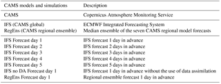
In early January 2017, severe winter weather struck several European regions, namely the Baltic Sea, northern Germany, Italy, the Balkan Peninsula and Turkey, with flooding, extreme cold and snow (Lentze, 2017). The international news media reported that at least 61 people died because of the extremely cold weather conditions in central, eastern and southern Europe (Associated Press, 2017). The prevailing synoptic conditions associated with these weather events are depicted in Fig. 1, which presents the temporal evolution (every 12 h) of IFS geopotential height, wind speed and wind direction at 300 hPa during the time period 3–9 January 2017. An upper level ridge gradually formed over the eastern Atlantic and western Europe in conjunction with a deep upper level trough over eastern and central Europe. Additionally, the jet stream was found on the western side of the upper level trough, with wind speeds occasionally exceeding 65 m s−1 (12:00 Z on 4 January 2017 and 00:00 Z on 5 January 2017). This synoptic situation resulted in the advection of very cold arctic air masses towards eastern, central and southern Europe and favoured the formation of tropopause folds along the path of the jet stream. In its later stage (00:00 Z on 8 January 2017 and after), the southernmost part of the system detached from the main stream, forming a cut-off low over the Balkans. The IFS temperatures at 850 hPa, averaged from 00:00 Z on 7 January to 21:00 Z on 10 January 2017, were below −14 ∘C in most of the Balkans, reaching values below −18 ∘C in the western Balkans (not shown). To stress the exceptional intensity of the cold intrusion, it is noted that the monthly mean climatological temperatures for January at 850 hPa, derived from ERA-Interim reanalyses for the 1981–2010 period, are not lower than −4 ∘C in the Balkan region (not shown).
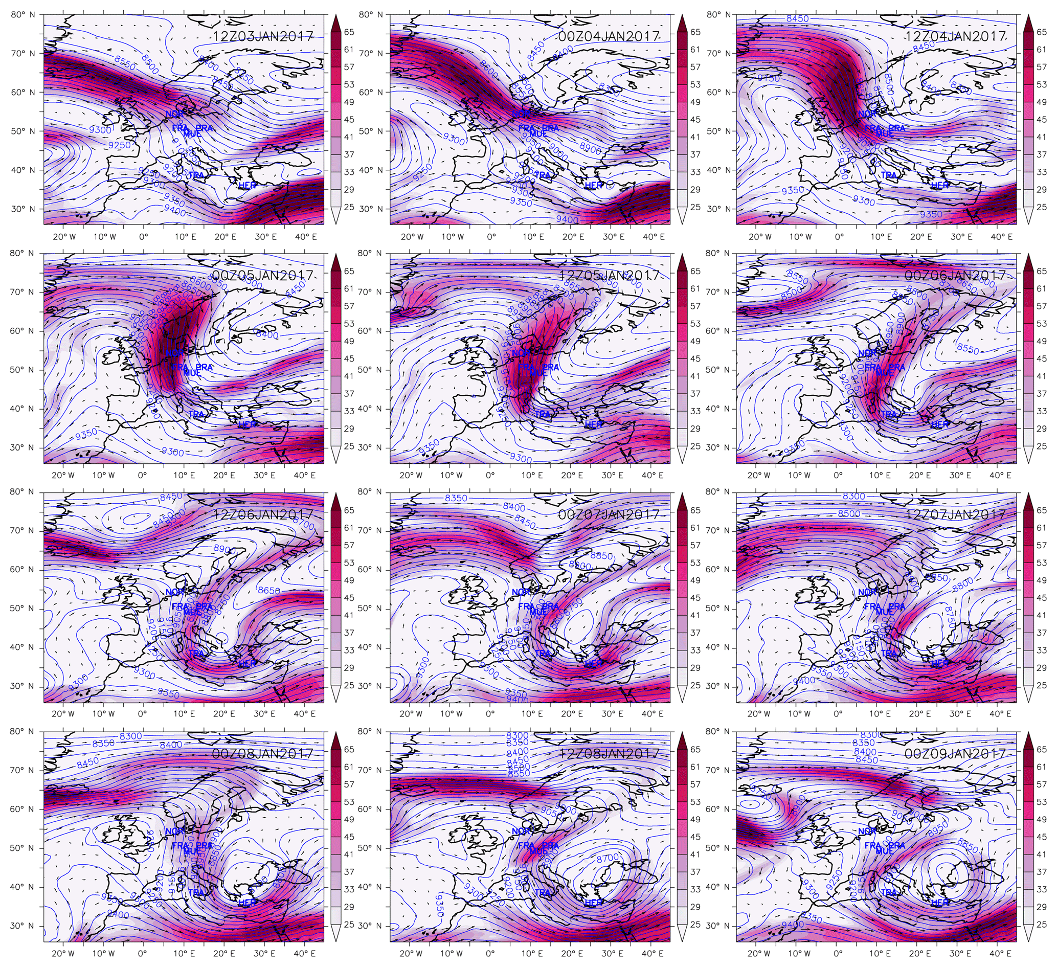
Figure 1IFS geopotential height (in gpm; contours), wind speed (in m s−1; colour shaded) and wind direction (vectors) at 300 hPa, during the period from 12:00 Z on 3 January 2017 to 00:00 Z on 9 January 2017 (12 h interval). Also shown are the locations of the observational sites (blue text) used in the study.
The horizontal thermal advection at 850 hPa was calculated at 3 h intervals, using the IFS data and employing second-order centred finite differences for the estimation of the horizontal derivatives. Cold advection at 850 hPa occurred in large parts of central, eastern and southern Europe in early January. Strong negative values of the horizontal thermal advection ( K hr−1) were exhibited continuously in large parts of Italy (5–7 January), the northern Balkans and central Europe (4–9 January), the western Balkans along the Adriatic coast (5–11 January) and northern Greece, southern FYROM (former Yugoslav Republic of Macedonia) and southwest Bulgaria (6–9 January). The latter maximum in cold advection resulted in a record period of 7 (5) consecutive days with frost (maximum daily temperature below 0 ∘C) from 6 to 12 (7 to 11) January at Thessaloniki (northern Greece), which is located a few metres above sea level.
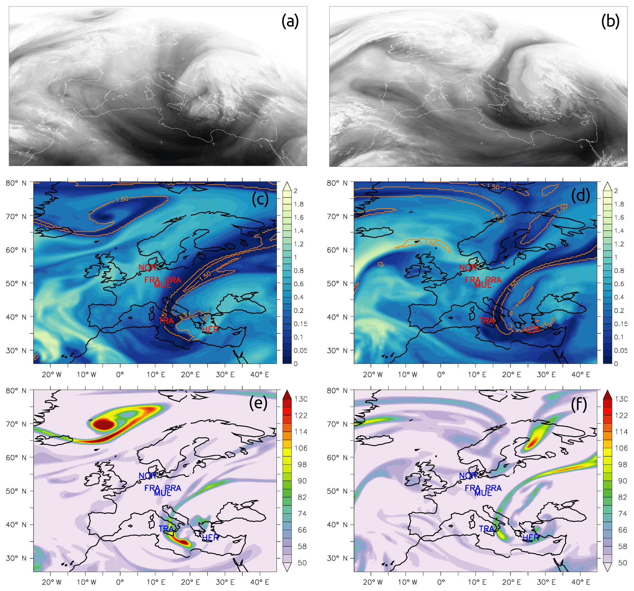
Figure 2Meteosat water vapour (5.35–7.15 µm) satellite images (a, b), IFS specific humidity (in g kg−1; colour shaded) and PV (1.5 pvu; contours) at 500 hPa (c, d), and IFS ozone mixing ratio (in ppb; colour shaded) at 500 hPa (e, f) at 12:00 Z on 6 January 2017 and 12:00 Z on 7 January 2017 respectively. Also shown are the locations of the observational sites (red and blue text) used in the study. Satellite images source: NERC Satellite Receiving Station, Dundee University, Scotland; http://www.sat.dundee.ac.uk/ (last access: 17 March 2017).
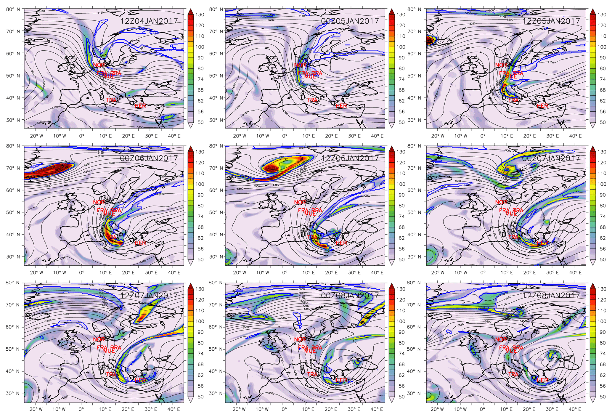
Figure 3IFS ozone mixing ratio (in ppb; colour shaded), geopotential height (in gpm, black contours) and PV (1.5 pvu; blue contours) at 500 hPa during the period from 12:00 Z on 4 January 2017 to 12:00 Z on 8 January 2017 (12 h interval). Also shown are the locations of the observational sites (red text) used in the study.

Figure 4RegEns ozone mixing ratio (in ppb; colour shaded) at 5000 m during the period from 12:00 Z on 4 January 2017 to 12:00 Z on 8 January 2017 (12 h interval). Also shown are the locations of the observational sites (blue text) used in the study.
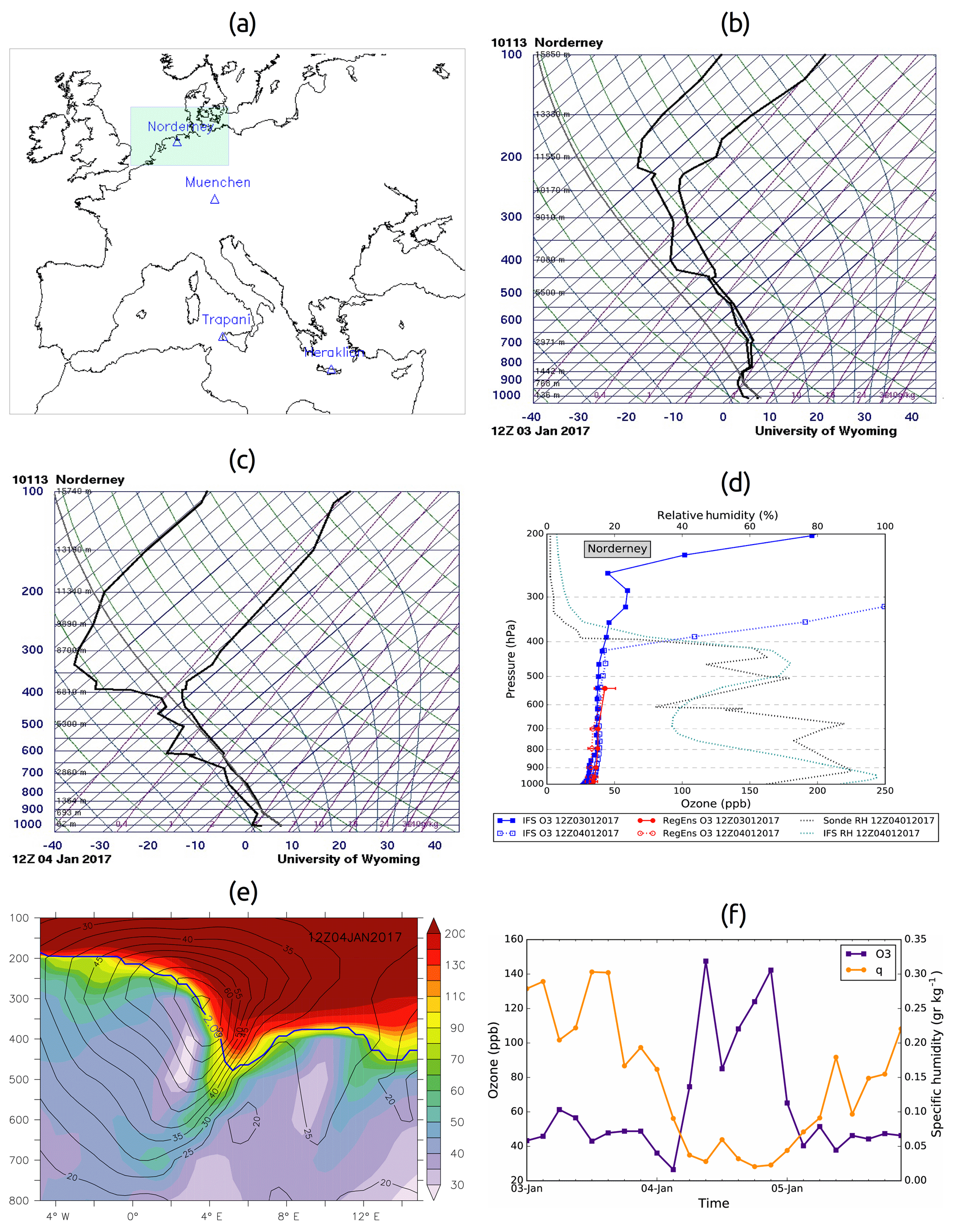
Figure 5(a) Norderney, Germany location. (b) Skew-T log-P diagrams at 12:00 Z on 3 January 2017 and (c) 12:00 Z on 4 January 2017. (d) Vertical profiles of IFS (blue) and RegEns (red) ozone mixing ratio (ppb) at 12:00 Z on 3 January 2017 (solid line) and 12:00 Z on 4 January 2017 (dashed line). The red bars denote the standard deviation among the regional ensemble members. Also shown are sonde (dashed black line) and IFS relative humidity (dashed cyan line) at 12:00 Z on 4 January 2017. (e) Longitude–pressure vertical cross section at 53.6∘ N of IFS ozone mixing ratio (in ppb; colour shaded), wind speed (in m s−1; black contours) and PV (2 pvu; blue contours) at 12:00 Z on 4 January 2017. (f) IFS ozone (blue) and specific humidity (orange) time series at 400 hPa.
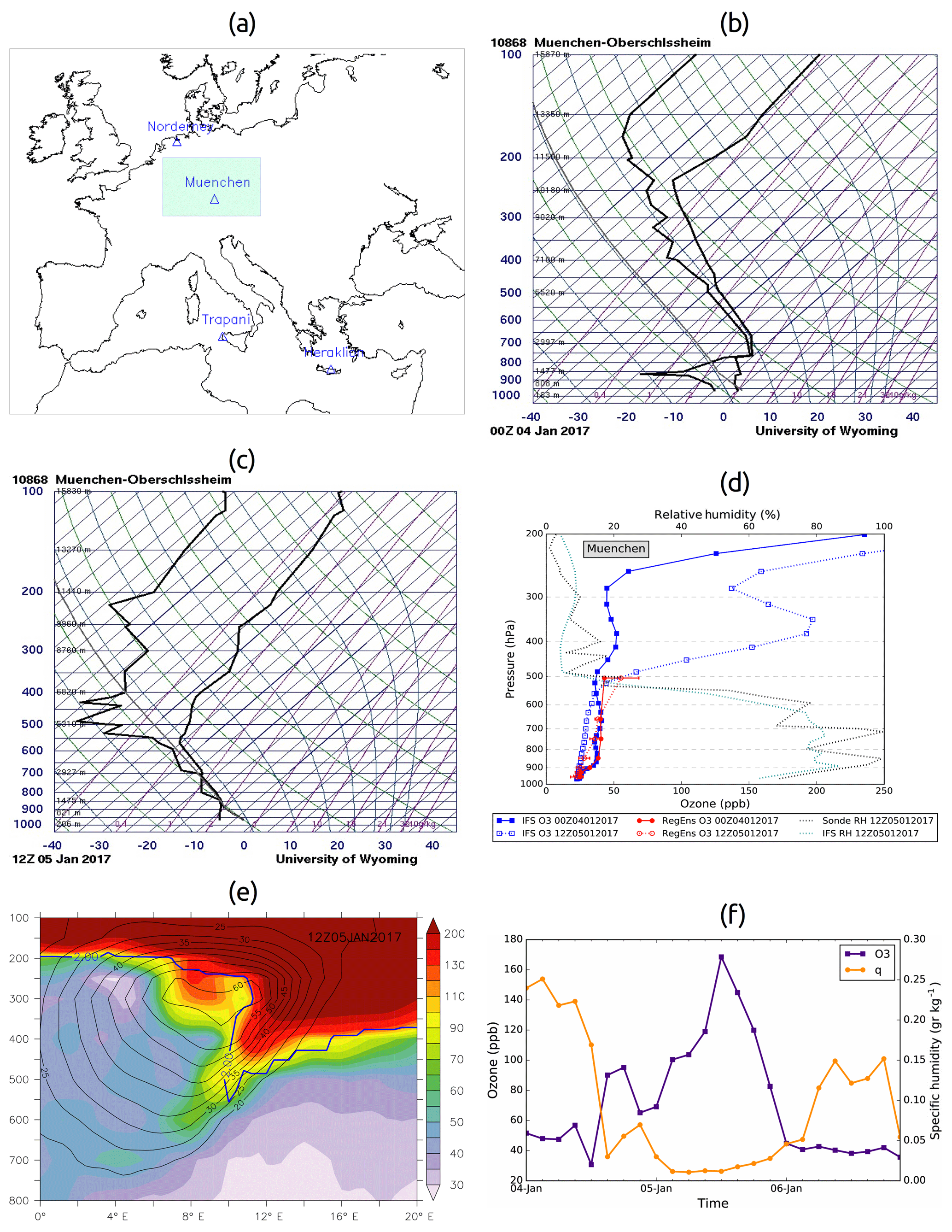
Figure 6(a) Muenchen, Germany location. (b) Skew-T log-P diagrams at 00:00 Z on 4 January 2017 and (c) 12:00 Z on 5 January 2017. (d) Vertical profiles of IFS (blue) and RegEns (red) ozone mixing ratio (ppb) at 00:00 Z on 4 January 2017 (solid line) and 12:00 Z on 5 January 2017 (dashed line). The red bars denote the standard deviation among the regional ensemble members. Also shown are sonde (dashed black line) and IFS relative humidity (dashed cyan line) at 12:00 Z on 5 January 2017. (e) Longitude–pressure vertical cross section at 48.4∘ N of IFS ozone mixing ratio (in ppb; colour shaded), wind speed (in m s−1; black contours) and PV (2 pvu; blue contours) at 12:00 Z on 5 January 2017. (f) IFS ozone (blue) and specific humidity (orange) time series at 400 hPa.
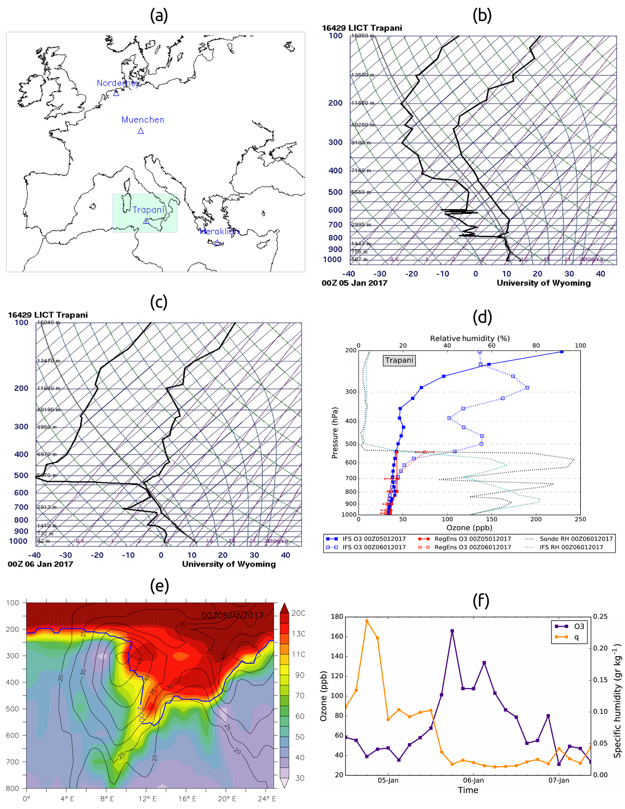
Figure 7(a) Trapani, Italy location. (b) Skew-T log-P diagrams at 00:00 Z on 5 January 2017 and (c) 00:00 Z on 6 January 2017. (d) Vertical profiles of IFS (blue) and RegEns (red) ozone mixing ratio (ppb) at 00:00 Z on 5 January 2017 (solid line) and 00:00 Z on 6 January 2017 (dashed line). The red bars denote the standard deviation among the regional ensemble members. Also shown are sonde (dashed black line) and IFS relative humidity (dashed cyan line) at 00:00 Z on 6 January 2017. (e) Longitude–pressure vertical cross section at 38∘ N of IFS ozone mixing ratio (in ppb; colour shaded), wind speed (in m s−1; black contours) and PV (2 pvu; blue contours) at 00:00 Z on 6 January 2017. (f) IFS ozone (blue) and specific humidity (orange) time series at 400 hPa.
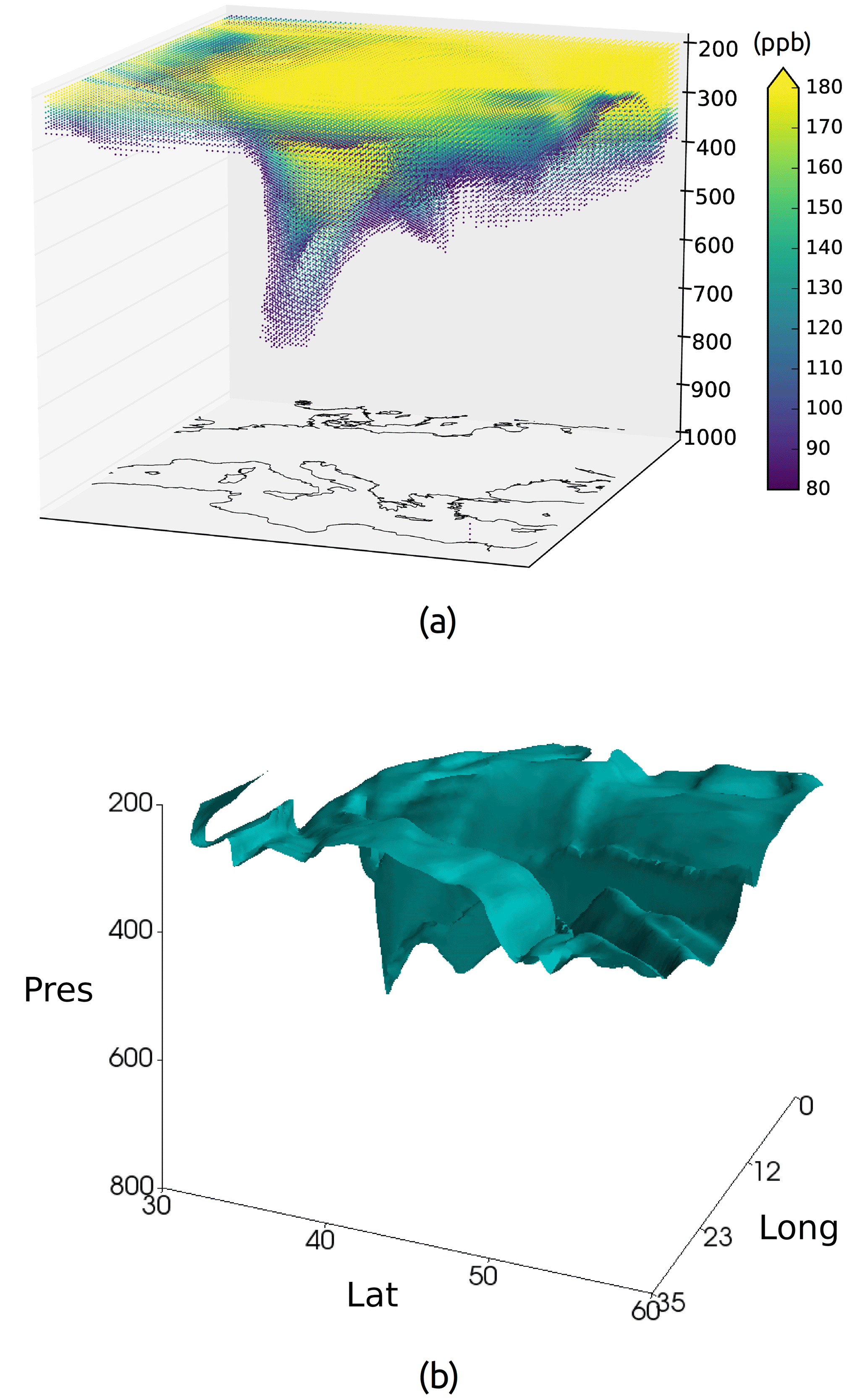
Figure 8(a) Three-dimensional (longitude, latitude, pressure (hPa)) spatial distribution of IFS ozone concentrations exceeding 80 ppb at 00:00 Z on 6 January 2017. (b) Three-dimensional (longitude, latitude, pressure (hPa)) IFS ozone concentrations' isosurface of 100 ppb at 00:00 Z on 6 January 2017.
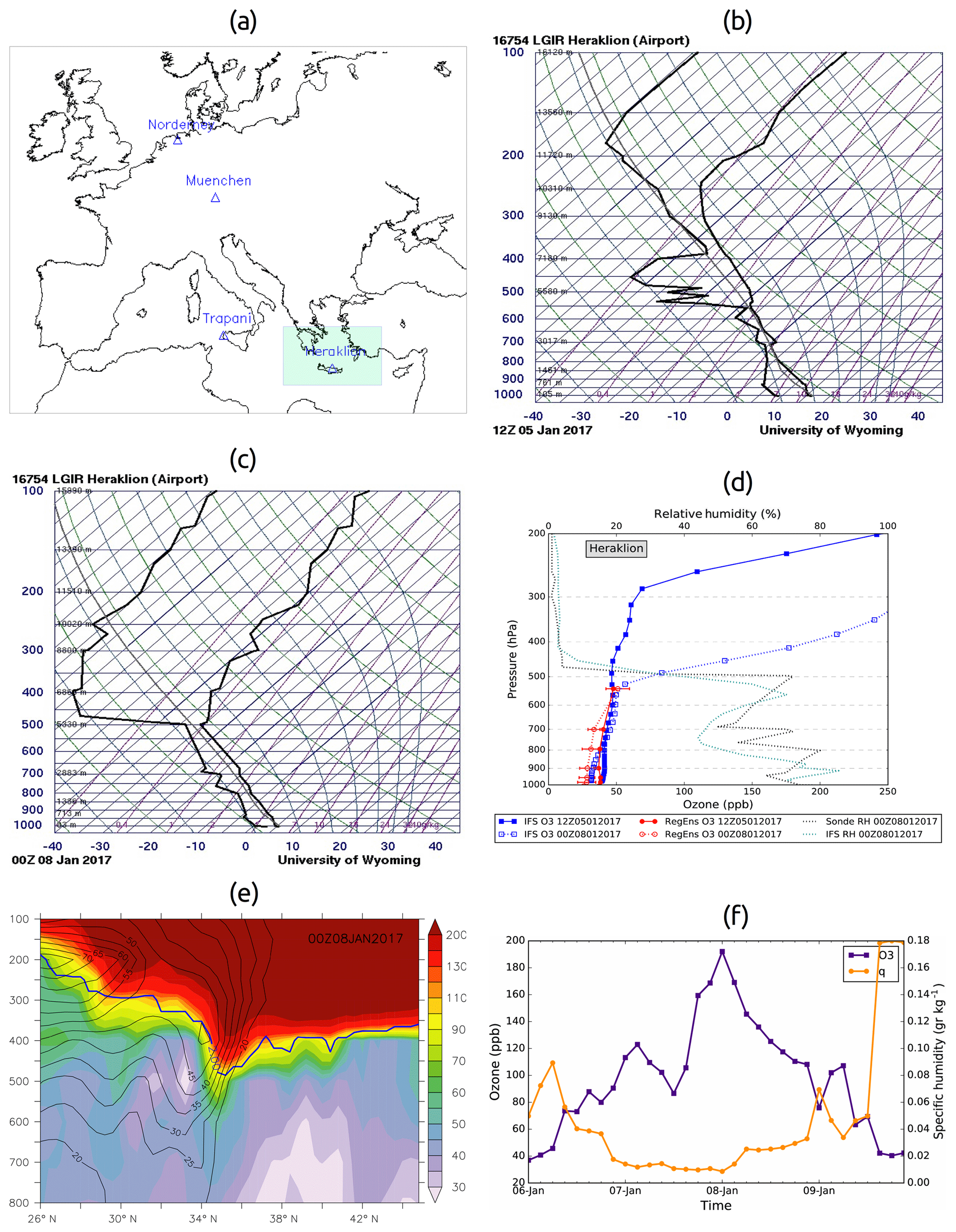
Figure 9(a) Heraklion, Greece location. (b) Skew-T log-P diagrams at 12:00 Z on 5 January 2017 and (c) 00:00 Z on 8 January 2017. (d) Vertical profiles of IFS (blue) and RegEns (red) ozone mixing ratio (ppb) at 12:00 Z on 5 January 2017 (solid line) and 00:00 Z on 8 January 2017 (dashed line). The red bars denote the standard deviation among the regional ensemble members. Also shown are sonde (dashed black line) and IFS relative humidity (dashed cyan line) at 00:00 Z on 8 January 2017. (e) Latitude–pressure vertical cross section at 25.2∘ E of IFS ozone mixing ratio (in ppb; colour shaded), wind speed (in m s−1; black contours) and PV (2 pvu; blue contours) at 00:00 Z on 8 January 2017. (f) IFS ozone (blue) and specific humidity (orange) time series at 400 hPa.
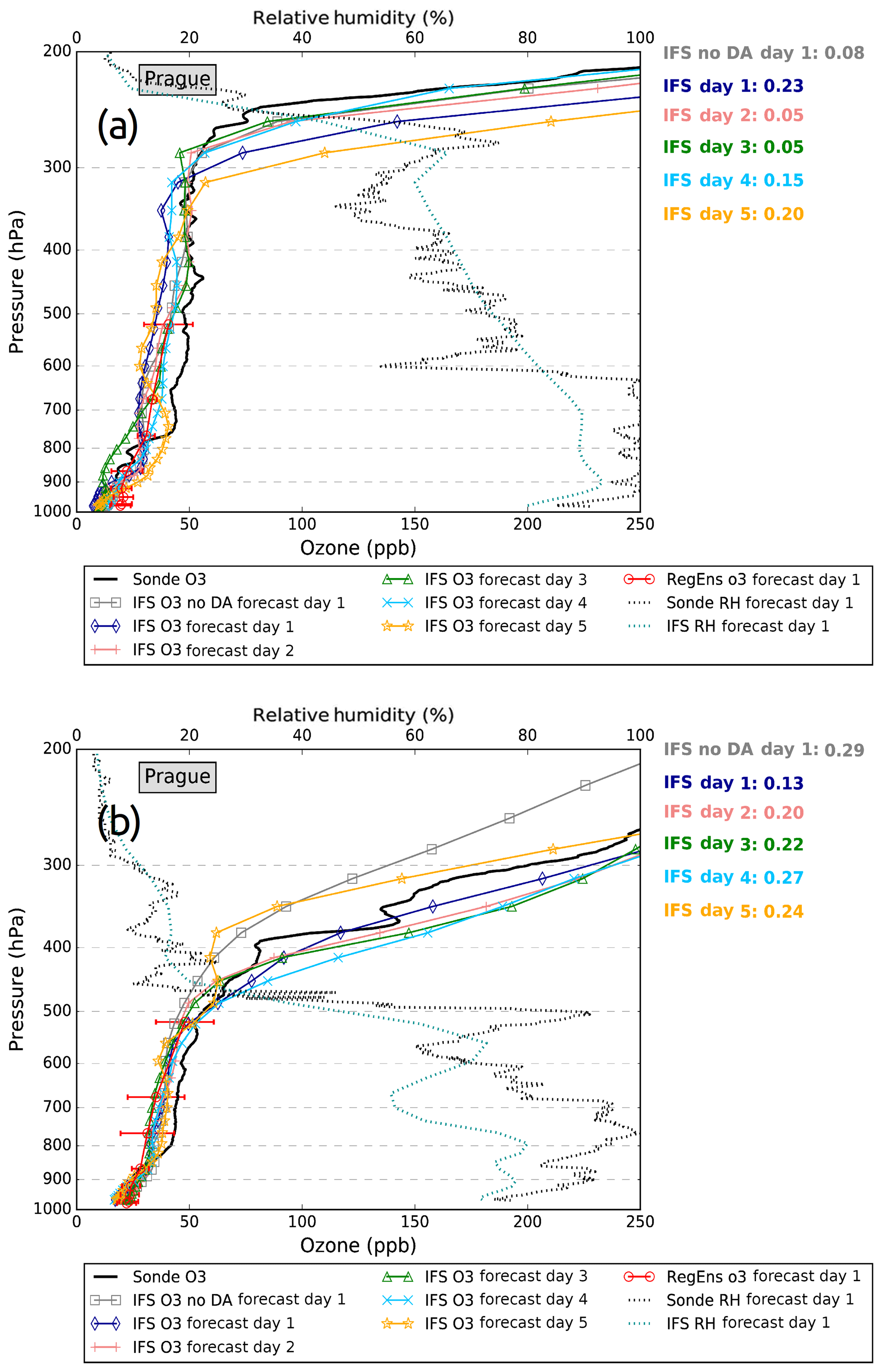
Figure 10Vertical profiles of ozone mixing ratio (ppb) over Prague, Czech Republic (14.44∘ E, 50∘ N), for ozonesondes (black line), IFS forecast day 1 (dark blue line), IFS forecast day 2 (coral line), IFS forecast day 3 (green line), IFS forecast day 4 (light blue line), IFS forecast day 5 (orange line), IFS no DA (without data assimilation) forecast day 1 (grey line) and RegEns (red line) at (a) 11:00 Z on 2 January 2017 and (b) 11:00 Z on 4 January 2017. Also shown are sonde (black dashed line) and IFS forecast day 1 relative humidity (cyan dashed line). The red bars denote the standard deviation among the regional ensemble members. The numbers on the right of the diagrams show the FGE values of IFS ozone (with the corresponding colour) at 300–500 hPa.
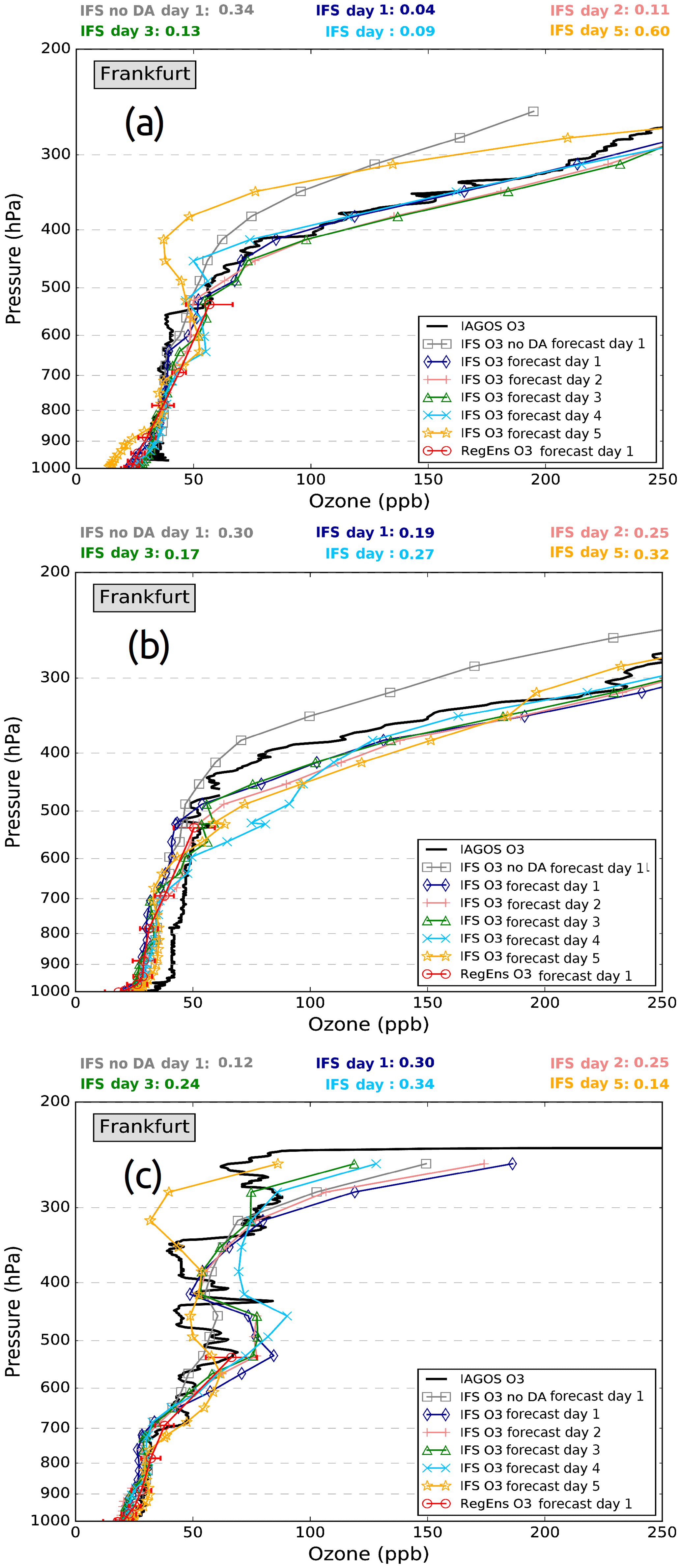
Figure 11Profiles of ozone mixing ratio (ppb) over the broader area of Frankfurt (8.5∘ E, 50∘ N) for IAGOS (black line), IFS forecast day 1 (dark blue line), IFS forecast day 2 (coral line), IFS forecast day 3 (green line), IFS forecast day 4 (light blue line), IFS forecast day 5 (orange line), IFS no DA (without data assimilation) forecast day 1 (grey line) and RegEns (red line) during (a) 13:00 Z on 4 January 2017, (b) 06:00 Z on 5 January 2017, and (c) 13:00 Z on 5 January 2017. The red bars denote the standard deviation among the regional ensemble members. The numbers above the diagrams show the FGE values of IFS ozone (with the corresponding colour) at 300–500 hPa (a, b) and 400–600 hPa (c).
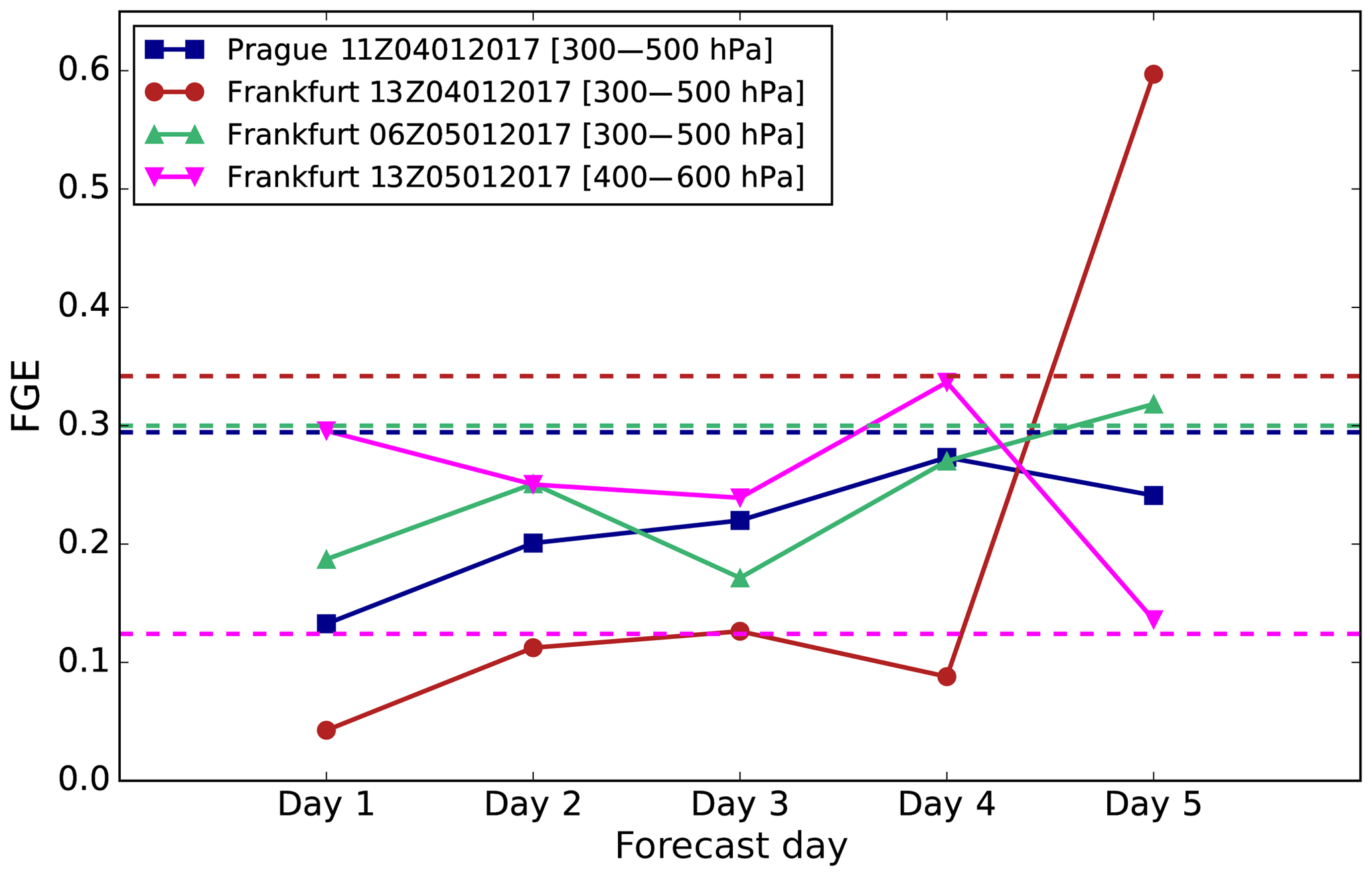
Figure 12FGE values of IFS ozone for forecast days 1–5 over Prague (11:00 Z on 4 January 2017) and Frankfurt (13:00 Z on 4 January 2017, 06:00 Z on 5 January 2017 and 13:00 Z on 5 January 2017). The dashed coloured horizontal lines represent the FGE values of IFS no DA ozone for forecast day 1.
To further explore the meteorological conditions and to investigate the case of stratospheric intrusions into the troposphere during the examined period, several stratospheric tracers are analysed from both IFS and observations. The water vapour satellite images at 12:00 Z on 6 and 7 January 2017, presented in Fig. 2a and b, respectively, display a “hook-shaped” streamer of dry air (dark shades) extending from north-eastern Europe to the central Mediterranean. This is a typical pattern encountered during STT events (Akritidis et al., 2010; Gerasopoulos et al., 2006; Zanis et al., 2003). The fields of IFS specific humidity at 500 hPa on the same days (Fig. 2c and d) resemble the observed satellite images. These depict a hook-shaped region of air with low specific humidity, affirming that the presence of dry air in the troposphere is captured well by the IFS global model. The respective PV isosurfaces of 1.5 pvu (Fig. 2c and d) overlap the band of dry air in the troposphere, while high ozone concentrations, up to 130 ppb, are also found over this dry streamer (Fig. 2e and f). Altogether, Fig. 2 indicates that this dry air with relatively high PV values and high ozone concentrations is of stratospheric origin.
3.2 Tropospheric ozone distribution in CAMS models
Figure 3 presents the evolution (12 h interval) of ozone concentrations exceeding 50 ppb, geopotential height and PV isosurfaces of 1.5 pvu from IFS at 500 hPa for the time period 4–8 January 2017, to examine ozone enhanced in the middle troposphere owing to STT in relation to the predominant synoptic–dynamic conditions. At 12:00 Z on 4 January 2017 a streamer of high ozone concentrations with values up to about 100 ppb is found over the Baltic Sea and northern Germany, near the ridge exit and trough entrance, where convergence and descending motions prevail, and in the vicinity of the jet stream (Fig. 1). During the next 24 h as the system moves further south, the streamer of high ozone concentrations crosses central Europe following the path of the jet stream. At 00:00 Z and 12:00 Z on 6 January 2017 ozone concentrations exceeding 130 ppb, linked with high PV values (>1.5 pvu), are found over the central Mediterranean, highlighting the vertical transport of ozone from the stratosphere down to the middle troposphere. During the next 48 h, the high ozone streamer moves further eastward, affecting the island of Crete (7 and 8 January 2017), and gradually dissipates.
In order to explore the capability of the regional models to reproduce the enhanced ozone seen in the mid-troposphere due to STT, the fields of RegEns ozone exceeding 50 ppb at 5000 m are shown in Fig. 4 for the same dates as in Fig. 3. Visual inspection of Fig. 4 indicates that the RegEns compares well with IFS as it synchronously captures the spatial distribution of ozone concentrations. In more detail, the hook-shaped patterns of high ozone are seen well in the CAMS regional product, with ozone mixing ratios exceeding 90 ppb at 12:00 Z on 6 January 2017 over the central Mediterranean. Although the spatio-temporal features of ozone in the RegEns agree well with that of the IFS, in quantitative terms, there are discrepancies between the regional and the global product. This is likely due to the fact that (a) the RegEns is presented at a 5000 m level (the uppermost level available) and the IFS at 500 hPa, (b) different resolution and advection schemes are used in global and regional models and (c) pressure and temperature values from the US Standard Atmosphere (USAF, 1976) were used for units' conversion in RegEns. Considering the ERA-Interim (Dee et al., 2011) temperatures during the period of interest for the units conversion may result in even lower RegEns ozone concentrations of up to ∼7 % in the regions exhibiting the lower temperatures (not shown). Overall, the agreement between the CAMS global and regional products highlights the critical role that the IFS boundary conditions and meteorological drivers play in the regional models for forecasting an STT event and the induced downward transport of ozone.
3.3 Vertical structure and analysis of STT event
Four sites are selected (Norderney, Germany; Muenchen, Germany; Trapani, Italy; Heraklion, Greece), located within the system transit path with available radiosonde observations, in order to study the vertical structure of the STT event and the subsequent transport of stratospheric ozone into the troposphere. To better depict the impact of STT on tropospheric ozone, two dates for analysis are selected for each site: one prior and one during the STT occurrence.
Starting from Norderney (see location in Fig. 5a), the skew-T log-P diagrams for 12:00 Z on 3 January 2017 and 12:00 Z on 4 January 2017 are presented in Fig. 5b and c, respectively. As can be seen from the comparison between the two figures, a distinct decrease of humidity (departure of dew-point curve (left) and temperature curve (right)) is found at 12:00 Z on 4 January 2017 between 250 and 400 hPa, while the tropopause drops to approximately 400 hPa. Furthermore, the vertical profile of the IFS ozone mixing ratio over Norderney during the examined dates (Fig. 5d) indicates a remarkable increase of ozone down to 400 hPa, verifying the aforementioned observed folding of the tropopause. The vertical profiles of the observed and IFS relative humidity (Fig. 5d) show a sharp decrease at 400 hPa, revealing that the intrusion of dry stratospheric air in the troposphere is captured well by the IFS. A comprehensive view of the induced stratospheric intrusion over Norderney is provided through the longitude–pressure cross section at 53.6∘ N, showing ozone, PV (2 pvu isosurface) and wind speed at 12:00 Z on 4 January 2017 (Fig. 5e). An impressive downward penetration of ozone-rich and PV-rich (>2 pvu) air down to approximately 600 hPa is found in the free troposphere and over the greater Norderney longitude band. The 2 pvu PV isosurface (dynamical tropopause; e.g. Hoskins et al., 1985) illustrates the tropopause folding on the right side of the jet stream (black contours) and down to 450 hPa at 5∘ E. The stratospheric origin of ozone in the upper troposphere over Norderney is also supported by the IFS ozone and specific humidity time series at 400 hPa, revealing a significant anti-correlation at the 95 % confidence level (Fig. 5f). The respective diagrams for Muenchen are presented in Fig. 6 for 00:00 Z on 4 January 2017 and 12:00 Z on 5 January 2017. Similarly, an intrusion of dry air is observed in the upper and middle troposphere (down to 550 hPa) at 12:00 Z on 5 January 2017 (Fig. 6b and c), which, along with the sharp increase/decrease of IFS ozone/relative humidity above 550 hPa (Fig. 6d), partially seen in RegEns ozone vertical profiles, indicates the downward transport of dry stratospheric air into the troposphere. The longitude–pressure cross section over Muenchen at 12:00 Z on 5 January 2017 (Fig. 6e) depicts the folding of the tropopause (2 pvu isosurface) in the vicinity of the jet stream and the associated vertical transport of ozone-rich air down to 600 hPa. In support of the above, the distinct increase of IFS ozone at 400 hPa is combined with a sharp decrease of IFS specific humidity (significant anti-correlation at the 95 % confidence level) (Fig. 6f).
A period of 12 h later (00:00 Z on 6 January 2017), and as the system moved further south, a dramatic decrease of humidity is observed in the middle troposphere and down to approximately 550 hPa over Trapani (Fig. 7b and c), with specific and relative humidity at 500 hPa dropping from 0.75 g kg−1 and 58 % (00:00 Z on 5 January) to 0.01 g kg−1 and 2 % (00:00 Z on 6 January 2017) respectively. The IFS specific humidity values at 500 hPa for the same dates are 0.49 and 0.025 g kg−1, respectively. On top of that, the vertical profiles of the observed and IFS relative humidity (Fig. 7d) indicate that the sharp decrease of humidity is reproduced well by the CAMS global model. The IFS system captures the dynamical features of the stratospheric intrusion as it is depicted in the vertical profiles of ozone, showing increased concentrations at 00:00 Z on 6 January 2017 down to 600 hPa, which is also seen in CAMS RegEns (Fig. 7d). The intense tropopause folding over Trapani is illustrated in Fig. 7e, with the dynamical tropopause dropping down to 550 hPa and ozone-rich air penetrating down to 800 hPa. Again, a significant anti-correlation at the 95 % confidence level is found between the IFS ozone and specific humidity time series at 400 hPa, indicating that the ozone increase results from the downward transport of ozone from the stratosphere (Fig. 7f). The three-dimensional field of IFS ozone concentrations exceeding 80 ppb at 00:00 Z on 6 January 2017 is presented in Fig. 8a, depicting the stratospheric ozone intrusion into the troposphere and over the broader Trapani region. The three-dimensional IFS ozone concentration isosurface of 100 ppb (Fig. 8b) resembles the folding of the tropopause along a north-east-oriented conceivable axis, which coincides with the high wind speed flow in the upper troposphere (Fig. 1). Later on and over Heraklion (see location in Fig. 9a), the skew-T log-P diagrams for 12:00 Z on 5 January 2017 and 00:00 Z on 8 January 2017 (Fig. 9b and c) and the respective vertical profiles of IFS ozone and relative humidity (Fig. 9d) reveal the presence of dry ozone-rich air in the upper and middle troposphere (down to 500 hPa). The increase in IFS ozone time series at 400 hPa is synchronized with the decrease of IFS specific humidity (significant anti-correlation at the 95 % confidence level), indicating that dry stratospheric air rich in ozone is transported into the troposphere over Heraklion (Fig. 9f). A more illustrative representation of the development and evolution of the examined STT event is provided in the three-dimensional animation (from 12:00 Z on 3 January 2017 to 21:00 Z on 8 January 2017 with 3 h interval) of IFS ozone concentrations exceeding 80 ppb in the Supplement.
3.4 Comparison with profile observations
In order to evaluate the forecasting capability of both IFS and RegEns regarding the downward transport of ozone during the examined STT event, we compare CAMS forecasts with profile observations from ozonesondes (WOUDC) and aircraft measurements (IAGOS). Two sites located across the passage of the examined system with available observational data during the examined period were selected: (a) Prague (ozonesondes) and (b) Frankfurt (aircraft measurements). The model error is quantified using the fractional gross error (FGE), which ranges between 0 and 2 and behaves symmetrically with respect to under- and overestimation:
where Mi represents the model value for level i, Oi is the corresponding observed value and N is the number of sample values.
Figure 10 displays the vertical profiles of observed and forecasted (IFS and RegEns) ozone concentrations over Prague at 11:00 Z (12:00 Z for CAMS models) on 2 January 2017 (prior the STT event) and 11:00 Z (12:00 Z for CAMS models) on 4 January 2017 (during the STT event). The intercomparison between the observed vertical profiles of ozone on the two dates indicates a distinct increase of ozone concentrations in the upper troposphere, probably related to the vertical transport of ozone from the stratosphere, reaching down to approximately 500 hPa. In support of the above findings, the respective vertical profiles of the observed and IFS relative humidity both show a distinct decrease at 500 hPa. Although the CAMS global model seems to underestimate (overestimate) ozone in (above) the free troposphere, the transition from the neutral condition to the STT event is captured well by the IFS day 1 forecast (Fig. 10), with an FGE value of 0.13 (300–500 hPa) on 4 January 2017. Whilst data assimilation resulted in overestimating ozone near the tropopause compared with the control run (Fig. 10a), it is clearly beneficial in reproducing the increase of ozone in the upper troposphere during the STT event (Fig. 10b). Notably, the respective FGE value for the control run at 4 January 2017 is 0.29, revealing an improvement in model performance due to data assimilation. Ozone in the RegEns forecast is higher within the planetary boundary layer than in IFS, with a relatively small spread among the RegEns members (Fig. 10a). In the free troposphere, the range of regional variability increases; however the RegEns remains close to the global forecast. The RegEns is also able to reproduce the ozone enhancement, following the IFS forecast closely (Fig. 10b). Day 1 to day 5 forecasts of IFS ozone indicate that the observed ozone increase in upper troposphere during the STT event is satisfactorily forecasted up to 3 days in advance, with FGE values not higher than 0.22 (Fig. 10b).
Three ozone profiles from aircraft measurements (two take-offs and one landing) over the broader region of Frankfurt at 13:00 Z on 4 January 2017, 6:00 Z on 5 January 2017 and 13:00 Z on 5 January 2017 are compared with the respective IFS and RegEns ozone profiles in Fig. 11. At 13:00 Z (12:00 Z for CAMS models) on 4 January 2017, the profile of the IFS ozone day 1 forecast is found to be in very good agreement with the IAGOS data, both depicting the increase of ozone down to approximately 500 hPa (Fig. 11a). The FGE was 0.04 for the 300–500 hPa altitude range. The respective profiles 17 h later (06:00 Z on 5 January 2017) also reveal enhanced ozone concentrations in the upper troposphere, which are captured by the IFS day 1 forecast (Fig. 11b) (FGE = 0.19 at 300–500 hPa). Finally, at 13:00 Z (12:00 Z for CAMS models) on 5 January 2017, the IFS day 1 forecast is found to overestimate the observed high ozone concentrations between 250 and 350 hPa, while it qualitatively captures the observed high ozone pattern in the middle troposphere between 400 and 600 hPa (Fig. 11c) (FGE = 0.30 at 400–600 hPa). The advantageous role of data assimilation can be affirmed from the intercomparison with the IFS control run, which exhibits FGE values of 0.34, 0.30 and 0.12 for the three dates respectively. A better agreement with observations is found for IFS when implementing data assimilation at 13:00 Z on 4 January 2017 and 06:00 Z on 5 January 2017 (Fig. 11a and b), while at 13:00 Z on 5 January 2017 (Fig. 11c), although the control run performs better in terms of bias, the data assimilation seems to help in the direction of reproducing the observed ozone peak in the middle troposphere. Concerning the RegEns, due to its limited vertical profile, up to about 550 hPa, the evaluation of its forecast performance is restricted. Nevertheless, there is a clear signal of increased ozone in the uppermost vertical level during all three dates. Regarding the forecast performance of CAMS global model, a relatively good agreement with observations is seen up to forecast day 3 at 13:00 Z on 4 January 2017 and 06:00 Z on 5 January 2017 (FGE values not higher than 0.25) (Fig. 11a and b), while at 13:00 Z on 5 January 2017 the observed ozone peak in the middle troposphere is somehow captured up to forecast day 3 but overestimated. Figure 12 depicts the FGE values of IFS ozone in relation to the forecast day for the observational instances of Prague and Frankfurt. Overall, a satisfactory forecast performance is revealed up to 3 days in advance with FGE values not higher than 0.3. Forecast day 1 exhibits the best agreement with observations, while after forecast day 3, more discrepancies are found between the forecast and the observations (see also Figs. 10 and 11).
We examined a deep STT event over Europe during the time period from 4 to 9 January 2017 in the CAMS global and regional forecast systems, assessing their capability to reproduce several key meteorological and chemical features of the event, with the aid of radiosonde, ozonesonde and aircraft observational data. The main results of the current study can be summarized as follows:
-
A deep upper level trough extending over central Europe favoured the development of tropopause folds and subsequently STT events along the jet stream axis at the west flank of the trough between 4 and 9 January 2017.
-
The hook-shaped streamer of dry stratospheric air in the middle troposphere seen in water vapour satellite images is reproduced well by the CAMS forecast systems, with tongues of anomalously high ozone concentrations in both CAMS global and regional models.
-
The observed (radiosondes) folding of the tropopause over various European sites is accurately reproduced by the CAMS global model. The vertical profiles and cross sections of IFS ozone and PV indicate that the vertical extent of the observed tropopause drop is well captured at all four of the sites studies.
-
The CAMS global system is found to be capable of capturing the evolution and vertical characteristics of the observed ozone field over Prague during the STT event. The observed ozone increase in the upper troposphere due to the stratospheric ozone downward transport is relatively well captured by the IFS. In addition, the global CAMS ozone forecasts in the greater Frankfurt area reveal an enhancement of ozone concentrations in the upper and middle troposphere as a result of the STT, which is in good agreement with the ozone measured by the IAGOS aircraft.
-
The evaluation of IFS ozone forecasts indicates that the CAMS global system is capable of forecasting the enhanced ozone concentrations during the STT event over Prague and Frankfurt up to 3 days in advance, both qualitatively and quantitatively.
-
Figures 10, 11 and 12 show that the use of data assimilation in the IFS is generally beneficial in forecasting the vertical and temporal variability of ozone during the examined STT event. Nevertheless, there are still discrepancies from the observations near the tropopause region as the sharp gradients around the tropopause are difficult to capture in global models (Clark et al., 2007; Gaudel et al., 2015).
-
Despite the limited vertical profile of RegEns forecast data, the CAMS regional models show an increase of ozone in the uppermost level for all instances in which the STT reached or exceeded that level.
Overall, this process-oriented analysis and evaluation study indicates that the CAMS global and regional forecast modelling systems are able to capture the specific regional meteorological and air quality characteristics of a specific deep STT event over Europe in January 2017. It also highlights the importance of data assimilation in the CAMS global model as well as of the meteorological and chemical forcing in the CAMS regional forecast systems.
The CAMS global and regional forecast data were processed within the framework of the service element CAMS_84. Both CAMS global and regional forecast products can be obtained from https://atmosphere.copernicus.eu/ (last access: 19 October 2018). The satellite images were obtained from the NERC Satellite Receiving Station, Dundee University, Scotland, at http://www.sat.dundee.ac.uk/ (last access: 17 March 2017). The radiosonde data were obtained from Wyoming University, Department of Atmospheric Science, at http://weather.uwyo.edu/upperair/sounding.html (last access: 27 April 2018). The ozonesonde data were obtained from the World Ozone and Ultraviolet Radiation Data Center (WOUDC) at https://woudc.org/ (last access: 9 June 2017). The IAGOS aircraft ozone measurements were provided by Hannah Clark (Hannah.Clark@aero.obs-mip.fr) and will shortly be available in the database at http://www.iagos.fr (last access: 19 October 2018) or directly via the AERIS website at http://www.aeris-data.fr (last access: 19 October 2018).
The supplement related to this article is available online at: https://doi.org/10.5194/acp-18-15515-2018-supplement.
DA, EK and PZ designed the study. EK collected the forecast data. DA performed the data analysis and wrote the paper. IP contributed to the synoptic analysis. JF and AI contributed to the IFS results' interpretation and JF performed the IFS control simulation without the use of data assimilation. HC provided the IAGOS aircraft measurements. HE is coordinating CAMS84 (global and regional a posteriori validation, including focus on the Arctic and Mediterranean areas). MP is coordinating CAMS50 (regional production). All authors contributed to interpretation of the results and the writing of the paper.
The authors declare that they have no conflict of interest.
This work is performed within the framework of the service element “CAMS_84:
Global and regional a posteriori validation, including focus on the Arctic
and Mediterranean areas” of the Copernicus Atmospheric Monitoring Services
(CAMS). ECMWF is the operator of CAMS on behalf of the European Union
(Delegation Agreement signed on 11 November 2014). The CAMS_84 work is financially
supported by ECMWF via its main contractor, Royal Netherlands Meteorological
Institute KNMI. The authors acknowledge the strong support of the European
Commission, Airbus and the Airlines (Lufthansa, Air-France, Austrian, Air
Namibia, Cathay Pacific, Iberia, China Airlines, Hawaiian Airlines so far)
who have carried the MOZAIC or IAGOS equipment and performed the maintenance since
1994. In its last 10 years of operation, MOZAIC has been funded by INSU-CNRS
(France), Météo-France, Université Paul Sabatier (Toulouse, France) and
Research Center Jülich (FZJ, Jülich, Germany). IAGOS has been
additionally funded by the EU projects IAGOS-DS and IAGOS-ERI. The
MOZAIC-IAGOS database is supported by AERIS (CNES and INSU-CNRS). Data are
also available via the AERIS website at https://www.aeris-data.fr (last access: 19 October 2018). The authors
acknowledge the use of Copernicus Atmosphere Monitoring Service Information (2017). We also acknowledge the WOUDC, the Department of Atmospheric Science
of Wyoming University and the NERC Satellite Receiving Station of Dundee University for the free use of ozonesonde data, radiosonde data and
satellite images respectively. AUTH (Aristotle University of Thessaloniki)
authors acknowledge the support of the scientific computing services of the
AUTH-IT Center (http://it.auth.gr, last access: 19 October 2018). Finally, the authors would like to
acknowledge the free use of Python (https://www.python.org, last access: 19 October 2018), Ferret
(http://ferret.pmel.noaa.gov/Ferret/, last access: 19 October 2018) and Mayavi
(Ramachandran and Varoquaux, 2011) software for the analysis and graphics of the
paper.
Edited by: Geraint
Vaughan
Reviewed by: two anonymous referees
Agusti-Panareda, A., Diamantakis, M., Bayona, V., Klappenbach, F., and Butz, A.: Improving the inter-hemispheric gradient of total column atmospheric CO2 and CH4 in simulations with the ECMWF semi-Lagrangian atmospheric global model, Geosci. Model Dev., 10, 1–18, https://doi.org/10.5194/gmd-10-1-2017, 2017. a
Akritidis, D., Zanis, P., Pytharoulis, I., Mavrakis, A., and Karacostas, T.: A deep stratospheric intrusion event down to the earth's surface of the megacity of Athens, Meteorol. Atmos. Phys., 109, 9–18, 2010. a, b
Akritidis, D., Pozzer, A., Zanis, P., Tyrlis, E., Škerlak, B., Sprenger, M., and Lelieveld, J.: On the role of tropopause folds in summertime tropospheric ozone over the eastern Mediterranean and the Middle East, Atmos. Chem. Phys., 16, 14025–14039, https://doi.org/10.5194/acp-16-14025-2016, 2016. a, b
Ambrose, J., Reidmiller, D., and Jaffe, D.: Causes of high O3 in the lower free troposphere over the Pacific Northwest as observed at the Mt. Bachelor Observatory, Atmos. Environ., 45, 5302–5315, 2011. a
Ancellet, G., Beekmann, M., and Papayannis, A.: Impact of a cutoff low development on downward transport of ozone in the troposphere, J. Geophys. Res.-Atmos., 99, 3451–3468, 1994. a
Appenzeller, C. and Davies, H.: Structure of stratospheric intrusions into the troposphere, Nature, 358, 570, https://doi.org/10.1038/358570a0, 1992. a, b
Appenzeller, C., Davies, H., and Norton, W.: Fragmentation of stratospheric intrusions, J. Geophys. Res.-Atmos., 101, 1435–1456, 1996. a
Associated Press: Europe cold snap: River shipping halted, death toll 61, https://apnews.com/25b99f47f5a3443ea19786226fd99920/schools-closed-free-buses-southern-poland-amid-smog (last access: 19 October 2018), 2017. a
Austin, J. and Follows, M.: The ozone record at Payerne: An assessment of the cross-tropopause flux, Atmos. Environ. A-Gen., 25, 1873–1880, 1991. a
Baray, J.-L., Daniel, V., Ancellet, G., and Legras, B.: Planetary-scale tropopause folds in the southern subtropics, Geophys. Res. Lett., 27, 353–356, 2000. a
Beekmann, M., Ancellet, G., Blonsky, S., De Muer, D., Ebel, A., Elbern, H., Hendricks, J., Kowol, J., Mancier, C., Sladkovic, R., Smit, H. G. J., Speth, P., Trickl, T., and Van Haver, P.: Regional and global tropopause fold occurrence and related ozone flux across the tropopause, J. Atmos. Chem., 28, 29–44, 1997. a
Benedetti, A., Morcrette, J.-J., Boucher, O., Dethof, A., Engelen, R. J., Fisher, M., Flentje, H., Huneeus, N., Jones, L., Kaiser, J. W., Kinne, S., Mangold, A., Razinger, M., Simmons, A. J., and Suttie, M.: Aerosol analysis and forecast in the European centre for medium-range weather forecasts integrated forecast system: 2. Data assimilation, J. Geophys. Res.-Atmos., 114, D13205, https://doi.org/10.1029/2008JD011115, 2009. a
Bithell, M., Vaughan, G., and Gray, L.: Persistence of stratospheric ozone layers in the troposphere, Atmos. Environ., 34, 2563–2570, 2000. a
Cariolle, D. and Déqué, M.: Southern Hemisphere medium-scale waves and total ozone disturbances in a spectral general circulation model, J. Geophys. Res.-Atmos., 91, 10825–10846, 1986. a
Cariolle, D. and Teyssèdre, H.: A revised linear ozone photochemistry parameterization for use in transport and general circulation models: multi-annual simulations, Atmos. Chem. Phys., 7, 2183–2196, https://doi.org/10.5194/acp-7-2183-2007, 2007. a
Clark, H., Cathala, M.-L., Teyssedre, H., Cammas, J.-P., and Peuch, V.-H.: Cross-tropopause fluxes of ozone using assimilation of MOZAIC observations in a global CTM, Tellus B, 59, 39–49, 2007. a
Cooper, O. R., Stohl, A., Hübler, G., Hsie, E. Y., Parrish, D. D., Tuck, A. F., Kiladis, G. N., Oltmans, S. J., Johnson, B. J., Shapiro, M., Moody, J. L., and Lefohn, A. S.: Direct transport of midlatitude stratospheric ozone into the lower troposphere and marine boundary layer of the tropical Pacific Ocean, J. Geophys. Res.-Atmos., 110, D23310, https://doi.org/10.1029/2005JD005783, 2005. a, b
Cooper, O. R., Oltmans, S. J., Johnson, B. J., Brioude, J., Angevine, W., Trainer, M., Parrish, D. D., Ryerson, T. R., Pollack, I., Cullis, P. D., Ives, M. A., Tarasick, D. W., Al-Saadi, J., and Stajner, I.: Measurement of western US baseline ozone from the surface to the tropopause and assessment of downwind impact regions, J. Geophys. Res.-Atmos., 116, D00V03, https://doi.org/10.1029/2011JD016095, 2011. a
Cristofanelli, P., Bonasoni, P., Tositti, L., Bonafe, U., Calzolari, F., Evangelisti, F., Sandrini, S., and Stohl, A.: A 6-year analysis of stratospheric intrusions and their influence on ozone at Mt. Cimone (2165 m above sea level), J. Geophys. Res.-Atmos., 111, D03306, https://doi.org/10.1029/2005JD006553, 2006. a, b
Cristofanelli, P., Bracci, A., Sprenger, M., Marinoni, A., Bonafè, U., Calzolari, F., Duchi, R., Laj, P., Pichon, J. M., Roccato, F., Venzac, H., Vuillermoz, E., and Bonasoni, P.: Tropospheric ozone variations at the Nepal Climate Observatory-Pyramid (Himalayas, 5079 m a.s.l.) and influence of deep stratospheric intrusion events, Atmos. Chem. Phys., 10, 6537–6549, https://doi.org/10.5194/acp-10-6537-2010, 2010. a
Crutzen, P. J.: Photochemical reactions initiated by and influencing ozone in unpolluted tropospheric air, Tellus, 26, 47–57, 1974. a
Danielsen, E. F.: Stratospheric-tropospheric exchange based on radioactivity, ozone and potential vorticity, J. Atmos. Sci., 25, 502–518, 1968. a
Danielsen, E. F. and Mohnen, V. A.: Project Dustorm report: Ozone transport, in situ measurements, and meteorological analyses of tropopause folding, J. Geophys. Res., 82, 5867–5877, 1977. a
Davies, T. and Schuepbach, E.: Episodes of high ozone concentrations at the earth's surface resulting from transport down from the upper troposphere/lower stratosphere: a review and case studies, Atmos. Environ., 28, 53–68, 1994. a
Dee, D. P., Uppala, S. M., Simmons, A. J., Berrisford, P., Poli, P., Kobayashi, S., Andrae, U., Balmaseda, M. A., Balsamo, G., Bauer, P., Bechtold, P., Beljaars, A. C. M., van de Berg, L., Bidlot, J., Bormann, N., Delsol, C., Dragani, R., Fuentes, M., Geer, A. J., Haimberger, L., Healy, S. B., Hersbach, H., Holm, E. V., Isaksen, L., Kallberg, P., Kohler, M., Matricardi, M., McNally, A. P., Monge-Sanz, B. M., Morcrette, J. J., Park, B. K., Peubey, C., de Rosnay, P., Tavolato, C., Thepaut, J. N., and Vitart, F.: The ERA-Interim reanalysis: Configuration and performance of the data assimilation system, Q. J. Roy. Meteor. Soc., 137, 553–597, 2011. a
Emery, C., Jung, J., Downey, N., Johnson, J., Jimenez, M., Yarwood, G., and Morris, R.: Regional and global modeling estimates of policy relevant background ozone over the United States, Atmos. Environ., 47, 206–217, 2012. a
Engelen, R. J., Serrar, S., and Chevallier, F.: Four-dimensional data assimilation of atmospheric CO2 using AIRS observations, J. Geophys. Res.-Atmos., 114, D03303, https://doi.org/10.1029/2008JD010739, 2009. a
Eskes, H., Huijnen, V., Arola, A., Benedictow, A., Blechschmidt, A.-M., Botek, E., Boucher, O., Bouarar, I., Chabrillat, S., Cuevas, E., Engelen, R., Flentje, H., Gaudel, A., Griesfeller, J., Jones, L., Kapsomenakis, J., Katragkou, E., Kinne, S., Langerock, B., Razinger, M., Richter, A., Schultz, M., Schulz, M., Sudarchikova, N., Thouret, V., Vrekoussis, M., Wagner, A., and Zerefos, C.: Validation of reactive gases and aerosols in the MACC global analysis and forecast system, Geosci. Model Dev., 8, 3523–3543, https://doi.org/10.5194/gmd-8-3523-2015, 2015. a
Fishman, J., Solomon, S., and Crutzen, P. J.: Observational and theoretical evidence in support of a significant in-situ photochemical source of tropospheric ozone, Tellus, 31, 432–446, 1979. a
Flemming, J., Inness, A., Flentje, H., Huijnen, V., Moinat, P., Schultz, M. G., and Stein, O.: Coupling global chemistry transport models to ECMWF's integrated forecast system, Geosci. Model Dev., 2, 253–265, https://doi.org/10.5194/gmd-2-253-2009, 2009. a
Flemming, J., Huijnen, V., Arteta, J., Bechtold, P., Beljaars, A., Blechschmidt, A.-M., Diamantakis, M., Engelen, R. J., Gaudel, A., Inness, A., Jones, L., Josse, B., Katragkou, E., Marecal, V., Peuch, V.-H., Richter, A., Schultz, M. G., Stein, O., and Tsikerdekis, A.: Tropospheric chemistry in the Integrated Forecasting System of ECMWF, Geosci. Model Dev., 8, 975–1003, https://doi.org/10.5194/gmd-8-975-2015, 2015. a, b, c, d
Follows, M. J. and Austin, J. F.: A zonal average model of the stratospheric contributions to the tropospheric ozone budget, J. Geophys. Res.-Atmos., 97, 18047–18060, 1992. a
Forster, C. and Wirth, V.: Radiative decay of idealized stratospheric filaments in the troposphere, J. Geophys. Res.-Atmos., 105, 10169–10184, 2000. a, b
Fuhrer, J., Skärby, L., and Ashmore, M. R.: Critical levels for ozone effects on vegetation in Europe, Environ. Pollut., 97, 91–106, 1997. a
Gaudel, A., Clark, H., Thouret, V., Jones, L., Inness, A., Flemming, J., Stein, O., Huijnen, V., Eskes, H., Nédélec P., and Boulangerand, D.: On the use of MOZAIC-IAGOS data to assess the ability of the MACC reanalysis to reproduce the distribution of ozone and CO in the UTLS over Europe, Tellus B, 67, 27955, https://doi.org/10.3402/tellusb.v67.27955, 2015. a
Gerasopoulos, E., Zanis, P., Papastefanou, C., Zerefos, C. S., Ioannidou, A., and Wernli, H.: A complex case study of down to the surface intrusions of persistent stratospheric air over the Eastern Mediterranean, Atmos. Environ., 40, 4113–4125, 2006. a, b
Guth, J., Josse, B., Marécal, V., Joly, M., and Hamer, P.: First implementation of secondary inorganic aerosols in the MOCAGE version R2.15.0 chemistry transport model, Geosci. Model Dev., 9, 137–160, https://doi.org/10.5194/gmd-9-137-2016, 2016. a
Hollingsworth, A., Engelen, R. J., Textor, C., Benedetti, A., Boucher, O., Chevallier, F., Dethof, A., Elbern, H., Eskes, H., Flemming, J., Granier, C., Kaiser, J. W., Morcrette, J. J., Rayner, P., Peuch, V. H., Rouil, L., Schultz, M. G., Simmons, A. J., and the GEMS Consortium: Toward a monitoring and forecasting system for atmospheric composition: The GEMS project, B. Am. Meteorol. Soc., 89, 1147–1164, 2008. a
Holton, J. R., Haynes, P. H., McIntyre, M. E., Douglass, A. R., Rood, R. B., and Pfister, L.: Stratosphere-troposphere exchange, Rev. Geophys., 33, 403–439, 1995. a, b
Hoskins, B. J., McIntyre, M., and Robertson, A. W.: On the use and significance of isentropic potential vorticity maps, Q. J. Roy. Meteor. Soc., 111, 877–946, 1985. a
Inness, A., Blechschmidt, A.-M., Bouarar, I., Chabrillat, S., Crepulja, M., Engelen, R. J., Eskes, H., Flemming, J., Gaudel, A., Hendrick, F., Huijnen, V., Jones, L., Kapsomenakis, J., Katragkou, E., Keppens, A., Langerock, B., de Mazière, M., Melas, D., Parrington, M., Peuch, V. H., Razinger, M., Richter, A., Schultz, M. G., Suttie, M., Thouret, V., Vrekoussis, M., Wagner, A., and Zerefos, C.: Data assimilation of satellite-retrieved ozone, carbon monoxide and nitrogen dioxide with ECMWF's Composition-IFS, Atmos. Chem. Phys., 15, 5275–5303, https://doi.org/10.5194/acp-15-5275-2015, 2015. a, b, c
Knowland, K., Ott, L., Duncan, B., and Wargan, K.: Stratospheric Intrusion-Influenced Ozone Air Quality Exceedances Investigated in the NASA MERRA-2 Reanalysis, Geophys. Res. Lett., 44, 10691–10701, https://doi.org/10.1002/2017GL074532, 2017. a
Kuenen, J. J. P., Visschedijk, A. J. H., Jozwicka, M., and Denier van der Gon, H. A. C.: TNO-MACC_II emission inventory; a multi-year (2003–2009) consistent high-resolution European emission inventory for air quality modelling, Atmos. Chem. Phys., 14, 10963–10976, https://doi.org/10.5194/acp-14-10963-2014, 2014. a
Lacis, A. A., Wuebbles, D. J., and Logan, J. A.: Radiative forcing of climate by changes in the vertical distribution of ozone, J. Geophys. Res.-Atmos., 95, 9971–9981, 1990. a
Lamarque, J.-F. and Hess, P. G.: Cross-tropopause mass exchange and potential vorticity budget in a simulated tropopause folding, J. Atmos. Sci., 51, 2246–2269, 1994. a
Langford, A., Masters, C., Proffitt, M., Hsie, E.-Y., and Tuck, A.: Ozone measurements in a tropopause fold associated with a cut-off low system, Geophys. Res. Lett., 23, 2501–2504, 1996. a
Langford, A., Brioude, J., Cooper, O., Senff, C., Alvarez, R., Hardesty, R., Johnson, B., and Oltmans, S.: Stratospheric influence on surface ozone in the Los Angeles area during late spring and early summer of 2010, J. Geophys. Res.-Atmos., 117, D00V06, https://doi.org/10.1029/2011JD016766, 2012. a
Lefohn, A. S., Wernli, H., Shadwick, D., Limbach, S., Oltmans, S. J., and Shapiro, M.: The importance of stratospheric–tropospheric transport in affecting surface ozone concentrations in the western and northern tier of the United States, Atmos. Environ., 45, 4845–4857, 2011. a
Lefohn, A. S., Wernli, H., Shadwick, D., Oltmans, S. J., and Shapiro, M.: Quantifying the importance of stratospheric-tropospheric transport on surface ozone concentrations at high-and low-elevation monitoring sites in the United States, Atmos. Environ., 62, 646–656, 2012. a
Lefohn, A. S., Emery, C., Shadwick, D., Wernli, H., Jung, J., and Oltmans, S. J.: Estimates of background surface ozone concentrations in the United States based on model-derived source apportionment, Atmos. Environ., 84, 275–288, 2014. a
Lelieveld, J. and Dentener, F. J.: What controls tropospheric ozone?, J. Geophys. Res.-Atmos., 105, 3531–3551, 2000. a
Lentze, G.: Newsletter No. 151 – Spring 2017. a
Lin, M., Fiore, A. M., Cooper, O. R., Horowitz, L. W., Langford, A. O., Levy, H., Johnson, B. J., Naik, V., Oltmans, S. J., and Senff, C. J.: Springtime high surface ozone events over the western United States: Quantifying the role of stratospheric intrusions, J. Geophys. Res.-Atmos., 117, D00V22, https://doi.org/10.1029/2012JD018151, 2012. a
Lin, M., Fiore, A. M., Horowitz, L. W., Langford, A. O., Oltmans, S. J., Tarasick, D., and Rieder, H. E.: Climate variability modulates western US ozone air quality in spring via deep stratospheric intrusions, Nat. Commun., 6, 7105, https://doi.org/10.1038/ncomms8105, 2015. a
Logan, J. A.: Tropospheric ozone: Seasonal behavior, trends, and anthropogenic influence, J. Geophys. Res.-Atmos., 90, 10463–10482, 1985. a
Marécal, V., Peuch, V.-H., Andersson, C., Andersson, S., Arteta, J., Beekmann, M., Benedictow, A., Bergström, R., Bessagnet, B., Cansado, A., Chéroux, F., Colette, A., Coman, A., Curier, R. L., Denier van der Gon, H. A. C., Drouin, A., Elbern, H., Emili, E., Engelen, R. J., Eskes, H. J., Foret, G., Friese, E., Gauss, M., Giannaros, C., Guth, J., Joly, M., Jaumouillé, E., Josse, B., Kadygrov, N., Kaiser, J. W., Krajsek, K., Kuenen, J., Kumar, U., Liora, N., Lopez, E., Malherbe, L., Martinez, I., Melas, D., Meleux, F., Menut, L., Moinat, P., Morales, T., Parmentier, J., Piacentini, A., Plu, M., Poupkou, A., Queguiner, S., Robertson, L., Rouïl, L., Schaap, M., Segers, A., Sofiev, M., Tarasson, L., Thomas, M., Timmermans, R., Valdebenito, Á., van Velthoven, P., van Versendaal, R., Vira, J., and Ung, A.: A regional air quality forecasting system over Europe: the MACC-II daily ensemble production, Geosci. Model Dev., 8, 2777–2813, https://doi.org/10.5194/gmd-8-2777-2015, 2015. a
Massart, S., Agustí-Panareda, A., Heymann, J., Buchwitz, M., Chevallier, F., Reuter, M., Hilker, M., Burrows, J. P., Deutscher, N. M., Feist, D. G., Hase, F., Sussmann, R., Desmet, F., Dubey, M. K., Griffith, D. W. T., Kivi, R., Petri, C., Schneider, M., and Velazco, V. A.: Ability of the 4-D-Var analysis of the GOSAT BESD XCO2 retrievals to characterize atmospheric CO2 at large and synoptic scales, Atmos. Chem. Phys., 16, 1653–1671, https://doi.org/10.5194/acp-16-1653-2016, 2016. a
Memmesheimer, M., Friese, E., Ebel, A., Jakobs, H., Feldmann, H., Kessler, C., and Piekorz, G.: Long-term simulations of particulate matter in Europe on different scales using sequential nesting of a regional model, Int. J. Environ. Pollut., 22, 108–132, 2004. a
Menut, L., Bessagnet, B., Khvorostyanov, D., Beekmann, M., Blond, N., Colette, A., Coll, I., Curci, G., Foret, G., Hodzic, A., Mailler, S., Meleux, F., Monge, J.-L., Pison, I., Siour, G., Turquety, S., Valari, M., Vautard, R., and Vivanco, M. G.: CHIMERE 2013: a model for regional atmospheric composition modelling, Geosci. Model Dev., 6, 981–1028, https://doi.org/10.5194/gmd-6-981-2013, 2013. a
Monks, P. S.: A review of the observations and origins of the spring ozone maximum, Atmos. Environ., 34, 3545–3561, 2000. a
Monks, P. S.: Gas-phase radical chemistry in the troposphere, Chem. Soc. Rev., 34, 376–395, 2005. a
Morcrette, J.-J., Boucher, O., Jones, L., Salmond, D., Bechtold, P., Beljaars, A., Benedetti, A., Bonet, A., Kaiser, J. W., Razinger, M., Schulz, M., Serrar, S., Simmons, A. J., Sofiev, M., Suttie, M., Tompkins, A. M., and Untch, A.: Aerosol analysis and forecast in the European Centre for medium-range weather forecasts integrated forecast system: Forward modeling, J. Geophys. Res.-Atmos., 114, D06206, https://doi.org/10.1029/2008JD011235, 2009. a
Nédélec, P., Blot, R., Boulanger, D., Athier, G., Cousin, J.-M., Gautron, B., Petzold, A., Volz-Thomas, A., and Thouret, V.: Instrumentation on commercial aircraft for monitoring the atmospheric composition on a global scale: the IAGOS system, technical overview of ozone and carbon monoxide measurements, Tellus B, 67, 27791, https://doi.org/10.3402/tellusb.v67.27791, 2015. a
Ordóñez, C., Brunner, D., Staehelin, J., Hadjinicolaou, P., Pyle, J., Jonas, M., Wernli, H., and Prévôt, A.: Strong influence of lowermost stratospheric ozone on lower tropospheric background ozone changes over Europe, Geophys. Res. Lett., 34, L07805, https://doi.org/10.1029/2006GL029113, 2007. a
Petzold, A., Thouret, V., Gerbig, C., Zahn, A., Brenninkmeijer, C. A. M., Gallagher, M., Hermann, M., Pontaud, M., Ziereis, H., Boulanger, D., Marshall, J., Nédélec, P., Smit, H. G. J., Friess, U., Flaud, J.-M., Wahner, A., Cammas, J.-P., Volz-Thomas, A. and IAGOS TEAM: Global-scale atmosphere monitoring by in-service aircraft–current achievements and future prospects of the European Research Infrastructure IAGOS, Tellus B, 67, 28452, https://doi.org/10.3402/tellusb.v67.28452, 2015. a
Price, J. and Vaughan, G.: The potential for stratosphere-troposphere exchange in cut-off-low systems, Q. J. Roy. Meteor. Soc., 119, 343–365, 1993. a
Ramachandran, P. and Varoquaux, G.: Mayavi: 3D visualization of scientific data, Comput. Sci. Eng., 13, 40–51, 2011. a
Robertson, L., Langner, J., and Engardt, M.: An Eulerian limited-area atmospheric transport model, J. Appli. Meteorol., 38, 190–210, 1999. a
Roelofs, G.-J. and Lelieveld, J.: Model study of the influence of cross-tropopause O3 transports on tropospheric O3 levels, Tellus B, 49, 38–55, 1997. a
Schaap, M., Timmermans, R. M., Roemer, M., Boersen, G., Builtjes, P., Sauter, F., Velders, G., and Beck, J.: The LOTOS-EUROS model: description, validation and latest developments, Int. J. Environ. Pollut., 32, 270–290, 2008. a
Shapiro, M.: Turbulent mixing within tropopause folds as a mechanism for the exchange of chemical constituents between the stratosphere and troposphere, J. Atmos. Sci., 37, 994–1004, 1980. a, b
Simpson, D., Benedictow, A., Berge, H., Bergström, R., Emberson, L. D., Fagerli, H., Flechard, C. R., Hayman, G. D., Gauss, M., Jonson, J. E., Jenkin, M. E., Nyíri, A., Richter, C., Semeena, V. S., Tsyro, S., Tuovinen, J.-P., Valdebenito, Á., and Wind, P.: The EMEP MSC-W chemical transport model – technical description, Atmos. Chem. Phys., 12, 7825–7865, https://doi.org/10.5194/acp-12-7825-2012, 2012. a
Škerlak, B., Sprenger, M., Pfahl, S., Tyrlis, E., and Wernli, H.: Tropopause Folds in ERA-Interim: Global Climatology and Relation to Extreme Weather Events, J. Geophys. Res.-Atmos.,120, 4860–4877, 2015. a, b
Sofiev, M., Vira, J., Kouznetsov, R., Prank, M., Soares, J., and Genikhovich, E.: Construction of the SILAM Eulerian atmospheric dispersion model based on the advection algorithm of Michael Galperin, Geosci. Model Dev., 8, 3497–3522, https://doi.org/10.5194/gmd-8-3497-2015, 2015. a
Solomon, S., Qin, D., Manning, M., Chen, Z., Marquis, M., Averyt, K., Tignor, M., and Miller, H. L.: IPCC, Climate change 2007: the physical science basis. Contribution of working group I to the fourth assessment report of the intergovernmental panel on climate change, 2007. a
Sprenger, M., Croci Maspoli, M., and Wernli, H.: Tropopause folds and cross-tropopause exchange: A global investigation based upon ECMWF analyses for the time period March 2000 to February 2001, J. Geophys. Res.-Atmos., 108, 8518, https://doi.org/10.1029/2002JD002587, 2003. a, b
Stohl, A., Spichtinger-Rakowsky, N., Bonasoni, P., Feldmann, H., Memmesheimer, M., Scheel, H., Trickl, T., Hübener, S., Ringer, W., and Mandl, M.: The influence of stratospheric intrusions on alpine ozone concentrations, Atmos. Environ., 34, 1323–1354, 2000. a, b
Stohl, A., Bonasoni, P., Cristofanelli, P., Collins, W., Feichter, J., Frank, A., Forster, C., Gerasopoulos, E., Gaggeler, H., James, P., Kentarchos, T., Kreipl, S., Kromp-Kolb, H., Kruger, B., sopoulos, Land, C., Meloen, J., Papayannis, A., Priller, A., Seibert, P., Sprenger, M., Roelofs, G. J., Scheel, E., Schnabel, C., Siegmund, P., Tobler, L., Trickl, T., Wernli, H., Wirth, V., Zanis, P., and Zerefos, C.: Stratosphere-troposphere exchange: A review, and what we have learned from STACCATO, J. Geophys. Res.-Atmos., 108, 8516, https://doi.org/10.1029/2002JD002490, 2003. a, b, c
Trickl, T., Feldmann, H., Kanter, H.-J., Scheel, H.-E., Sprenger, M., Stohl, A., and Wernli, H.: Forecasted deep stratospheric intrusions over Central Europe: case studies and climatologies, Atmos. Chem. Phys., 10, 499–524, https://doi.org/10.5194/acp-10-499-2010, 2010. a
Trickl, T., Bärtsch-Ritter, N., Eisele, H., Furger, M., Mücke, R., Sprenger, M., and Stohl, A.: High-ozone layers in the middle and upper troposphere above Central Europe: potential import from the stratosphere along the subtropical jet stream, Atmos. Chem. Phys., 11, 9343–9366, https://doi.org/10.5194/acp-11-9343-2011, 2011. a
Tyrlis, E., Škerlak, B., Sprenger, M., Wernli, H., Zittis, G., and Lelieveld, J.: On the linkage between the Asian summer monsoon and tropopause fold activity over the eastern Mediterranean and the Middle East, J. Geophys. Res.-Atmos., 119, 3202–3221, 2014. a
USAF, U.: Standard atmosphere, 1976, NASA TMX-74335, 12–15, 1976. a
Vaughan, G., Price, J., and Howells, A.: Transport into the troposphere in a tropopause fold, Q. J. Roy. Meteor. Soc., 120, 1085–1103, 1994. a
WHO: Health aspects of air pollution with particulate matter, ozone and nitrogen dioxide, Copenhagen: WHO Regional Office for Europe, Bonn, 2003. a
Wimmers, A. J., Moody, J. L., Browell, E. V., Hair, J. W., Grant, W. B., Butler, C. F., Fenn, M. A., Schmidt, C. C., Li, J., and Ridley, B. A.: Signatures of tropopause folding in satellite imagery, J. Geophys. Res.-Atmos., 108, 8360, https://doi.org/10.1029/2001JD001358, 2003. a
Wirth, V.: Diabatic heating in an axisymmetric cut-off cyclone and related stratosphere-troposphere exchange, Q. J. Roy. Meteor. Soc., 121, 127–147, 1995. a
WMO/GAW Ozone Monitoring Community: World Meteorological Organization-Global Atmosphere Watch Program (WMO-GAW)/World Ozone and Ultraviolet Radiation Data Centre (WOUDC) [Data], alist of all contributors is available on the website, https://doi.org/10.14287/10000001, available at: http://woudc.org, last access: 9 June 2017. a
Zanis, P., Trickl, T., Stohl, A., Wernli, H., Cooper, O., Zerefos, C., Gaeggeler, H., Schnabel, C., Tobler, L., Kubik, P. W., Priller, A., Scheel, H. E., Kanter, H. J., Cristofanelli, P., Forster, C., James, P., Gerasopoulos, E., Delcloo, A., Papayannis, A., and Claude, H.: Forecast, observation and modelling of a deep stratospheric intrusion event over Europe, Atmos. Chem. Phys., 3, 763–777, https://doi.org/10.5194/acp-3-763-2003, 2003. a, b
Zanis, P., Hadjinicolaou, P., Pozzer, A., Tyrlis, E., Dafka, S., Mihalopoulos, N., and Lelieveld, J.: Summertime free-tropospheric ozone pool over the eastern Mediterranean/Middle East, Atmos. Chem. Phys., 14, 115–132, https://doi.org/10.5194/acp-14-115-2014, 2014. a, b
Zhang, L., Jacob, D. J., Downey, N. V., Wood, D. A., Blewitt, D., Carouge, C. C., van Donkelaar, A., Jones, D. B., Murray, L. T., and Wang, Y.: Improved estimate of the policy-relevant background ozone in the United States using the GEOS-Chem global model with horizontal resolution over North America, Atmos. Environ., 45, 6769–6776, 2011. a
https://atmosphere.copernicus.eu/ (last access: 19 October 2018)