the Creative Commons Attribution 4.0 License.
the Creative Commons Attribution 4.0 License.
 | 22 Oct 2018
Evaluating cloud properties in an ensemble of regional online coupled models against satellite observations
Rocío Baró
Pedro Jiménez-Guerrero
Martin Stengel
Dominik Brunner
Gabriele Curci
Renate Forkel
Lucy Neal
Laura Palacios-Peña
Nicholas Savage
Martijn Schaap
Paolo Tuccella
Hugo Denier van der Gon
Stefano Galmarini
Online coupled meteorology–chemistry models permit the description of the aerosol–radiation (ARI) and aerosol–cloud interactions (ACIs). The aim of this work is to assess the representation of several cloud properties in regional-scale coupled models when simulating the climate–chemistry–cloud–radiation system. The evaluated simulations are performed under the umbrella of the Air Quality Model Evaluation International Initiative (AQMEII) Phase 2 and include ARI+ACI interactions. Model simulations are evaluated against observational data from the European Space Agency (ESA) Cloud_cci project. The results show an underestimation (overestimation) of cloud fraction (CF) over land (sea) areas by the models. Lower bias values are found in the ensemble mean. Cloud optical depth (COD) and cloud ice water path (IWP) are generally underestimated over the whole European domain. The cloud liquid water path (LWP) is broadly overestimated. The temporal correlation suggests a generally positive correlation between models and satellite observations. Finally, CF gives the best spatial variability representation, whereas COD, IWP, and LWP show less capacity. The differences found can be attributed to differences in the microphysics schemes used; for instance, the number of ice hydrometeors and the prognostic/diagnostic treatment of the LWP are relevant.


Atmospheric aerosols vary in time and space, influence the Earth's radiation budget, and can lead to variations in cloud microphysics, which impact cloud radiative properties and climate. These processes have traditionally been called the aerosol direct effect but were renamed after the Fifth Report of the Intergovernmental Panel on Climate Change (IPCC AR5) (Boucher et al., 2013; Myhre et al., 2013) as aerosol–radiation interactions (ARI). Furthermore, aerosols serve as cloud condensation nuclei (CCN) that influence overall cloud radiative properties through interactions referred to as the first indirect effect or Twomey effect (Twomey, 1974, 1977). More aerosol particles lead to more cloud condensation nuclei, which results in an increased concentration of cloud droplets. When the cloud water is fixed, it is accompanied by a reduced cloud droplet size and increased cloud reflectivity. Altogether, this results in less solar energy absorbed and a cooling of the system. Aerosols that act as CCN may affect precipitation efficiency, cloud lifetime, and cloud thickness and could thus further influence weather and climate through the second indirect effect (Albrecht, 1989), also known as the cloud lifetime effect. The modification of cloud microphysical properties is expected to have an impact on the cloud evolution, particularly in terms of a cloud's ability to generate large enough droplets to initiate precipitation. This effect is traditionally called the second aerosol indirect effect, but since the AR5, these indirect effects are called aerosol–cloud interactions (ACIs). Those interactions are more uncertain due to the complexity of the microphysical processes (Boucher and Lohmann, 1995; Lohmann and Feichter, 2005; Schwartz et al., 2002).
The inclusion of aerosol interactions in air quality/climate modelling is an important challenge and is also important for the development of integrated emissions control strategies for both air quality management and climate change mitigation (Rosenfeld et al., 2014; Yu et al., 2014). There are different approaches to address the study of ACI, usually by combining methodologies of observations and/or modelling. In the field of observations/remote sensing, McComiskey et al. (2009) used atmospheric radiation measurement (ARM) focused on the California area. These authors studied the albedo effect as the change in cloud droplet number concentration (CDNC) with aerosol concentration, which resulted in local radiative forcing of around −13 W m−2 (top of the atmosphere). Liu et al. (2011) also used ARM combined with GOES satellite measurements and theoretically derived an analytical relationship, linking relative surface shortwave cloud radiative forcing, cloud fraction, and cloud albedo. They noticed its utility for diagnosing deficiencies of cloud–radiation parameterizations in climate models. By using observations and modelling, Avey et al. (2007) employed cloud retrievals from the Moderate Resolution Imaging Spectroradiometer (MODIS) and output from a tracer transport model (FLEXPART). They compared cloud and pollution fields on the northeastern coast of the United States, during 2004, under the umbrella of the International Consortium for Atmospheric Research on Transport and Transformation (ICARTT) mission. They found that, where the transport model indicated polluted air, cloud droplet effective radii were smaller, while cloud optical depth (COD) was greater in some cases or at least close to the primary source regions. They found no conclusive evidence for the perturbation of the cloud liquid water path (LWP) by pollution. Yang et al. (2011) used the Weather Research Forecast coupled with a chemistry (WRF-Chem) model in a study conducted over the northern Chilean and southern Peruvian coasts from 15 October to 16 November 2008. They ran a simulation including ACI and compared it to other runs with fixed CDNC and simplified cloud and aerosol treatments. They found that the coupled simulation of ACI improved cloud optical and microphysical properties.
In order to realistically simulate the chemistry–aerosol–cloud–radiation–climate interactions, fully online-coupled meteorology–atmospheric-chemistry models are needed (Baklanov et al., 2008; Zhang, 2008). Moreover, to build confidence in air-quality–climate interaction studies, a thorough evaluation is needed on both global and regional scales. Particularly, ACI is still considered one of the most important uncertainties in anthropogenic climate perturbations (Penner et al., 2006; Quaas et al., 2009). The Air Quality Model Evaluation International Initiative (AQMEII) (Rao et al., 2011) was set up to promote research into regional air quality model evaluations across the regional modelling communities in Europe and North America. This study is conducted in the context of Phase 2 of AQMEII where model evaluation is made in online-coupled air quality models. An extensive model evaluation of the simulations shown herein can be found in Brunner et al. (2015) and in Im et al. (2015a) and Im et al. (2015b). There is a follow-up of the AQMEII initiative, Phase 3, which focuses on evaluating and intercomparing regional and linked global/regional modelling systems by collaborating with the Task Force on Hemispheric Transport of Air Pollution, Phase 2 (Janssens-Maenhout et al., 2015).
To the authors' knowledge, apart from the study of Makar et al. (2015a), there are no other studies that have taken into account ARI+ACI in regional coupled models. The main objective of this contribution is to assess the representation of several cloud variables in different regional-scale integrated models when simulating ARI+ACI. To date, all the collective studies performed used global models and regional climate analyses do not usually bear in mind ARI+ACI. In the next section, we explain the methodology followed, where we provide an overview of the model simulations, the description of the observational data used, and the evaluation methodology. In Sect. 3, the results of the evaluation of the assessed cloud properties and the spatial correlation and variability are described. The paper closes with a summary and conclusions.
This section describes the strategies adopted to analyse cloud properties in online-coupled models. As stated in the introduction, the analysed model outputs are the results run according to the AQMEII Phase 2 initiative. In order to analyse the capacities of the coupled models which take into account ARI+ACI, simulations from different models with identical meteorological boundary conditions and anthropogenic emissions have been analysed.
The common set-up for the participating models and a unified output strategy allowed us to analyse the representation of model output in relation to similarities and differences in the model's response to the aerosol–radiation and aerosol–cloud interactions. The studied variables are the cloud fraction (CF), the cloud optical depth (COD), the cloud ice path (IWP), and the cloud water path (LWP). The target domain is Europe, and the analysis covers the year 2010 and its seasonality.
2.1 Model simulations
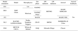
Table 1 offers an overview of the 1-year model simulations that contribute to this study in the AQMEII Phase 2 context. It includes five simulations conducted with the following online-coupled models: LOTOS-EUROS (NL2; Sauter et al., 2012), UKCA (UK4; Savage et al., 2013), and WRF-Chem (ES1, DE4, and IT2; Grell and Baklanov, 2011; Grell et al., 2005). LOTOS-EUROS is a semi-online model where the two models run separately but wait for one another to exchange information (meteorology and aerosol concentrations) every 3 h. Cloud fields were an optional part of the variables to be submitted and not all models were able to provide all these fields within the limited time available. Of the 13 models in AQMEII 2 which modelled the European domain, only 5 provided any of these fields and only 3 presented a complete set. To facilitate the cross-comparison between models, the participating groups interpolated their model output to a common grid at the 0.25∘ resolution (except for NL2 model, which had a smaller grid).
All the simulations were driven by the European Centre for Medium-Range Weather Forecasts (ECMWF) operational analyses (with data at 00:00 and 12:00 UTC) and with respective forecasts (at 3/6/9, etc., hours), so that the time interval of meteorological fields used for the boundary conditions was 3 hourly. The chemical initial conditions (ICs) were provided by the ECMWF IFS-MOZART model. The anthropogenic emissions employed were provided by the Netherlands Organization for Applied Scientific Research (TNO). The dataset is a follow-on to the widely used TNO-MACC database (Pouliot et al., 2012). Biogenic emissions were estimated by the Model of Emissions of Gases and Aerosols from Nature (MEGAN) (Guenther et al., 2006), which were calculated online. Fire emissions data were obtained from the IS4FIRE Project (http://is4fires.fmi.fi, last access: 15 January 2017). The emission dataset is estimated by a reanalysis of the fire radiative power data obtained by the MODIS instrument onboard the Aqua and Terra satellites. For further information about the models' parameterizations, the reader is referred to Brunner et al. (2015) and Im et al. (2015a, b).
2.2 Observational data
In order to analyse the representation of the different cloud properties, model data were compared and evaluated against the satellite-based observations of cloud properties. In more detail, the satellite data were generated by the European Space Agency (ESA) Cloud_cci project, within the ESA's Climate Change Initiative (CCI) programme (Hollmann et al., 2013). Several datasets are generated in Cloud_cci (Stengel et al., 2017a), and in this study, the Level-3C data (monthly averages and histograms) of the Cloud_cci AVHRR-PM dataset (Stengel et al., 2017b) were used. Data were retrieved by employing the Community Cloud retrieval for Climate (McGarragh et al., 2018; Sus et al., 2018) using measurements of the Advanced Very High Resolution Radiometer (AVHRR) onboard the National Oceanic and Atmospheric Administration satellite no. 19 (NOAA-19). CC4CL itself consists of three parts: cloud detection, cloud phase assignment, and the retrieval of cloud properties (e.g. optical thickness and effective radius). For the latter, scattering properties of liquid clouds are determined following Mie theory code as implemented by Grainger et al. (2004) using a modified gamma distribution to which the effective radius, which parameterizes the size distribution, is related. For ice clouds, the ice crystal single-scattering models of Baum et al. (2011, 2014) are used, with the bulk single-scattering properties being determined by an integration over particle size distribution of nine ice particle habits. For more information, see McGarragh et al. (2018).
The Level 3C data were used in this study, which have a spatial resolution of 0.5∘ latitude/longitude and represents a monthly mean of instantaneous cloud property retrievals taken at 01:30 and 13:30. The dataset version used was v2.2, which contained two significant bug fixes compared to Stengel et al. (2017a), who described v2.0: (1) correcting a miscalculation of the bidirectional reflectance distribution function (BRDF) components under the condition of high solar zenith angles and/or snow/ice-covered surfaces; (2) correcting lookup tables with precalculated radiances according to ice cloud properties, as well as viewing geometry and illumination conditions. Both bug fixes lead to a significant reduction in the random and systematic uncertainties of the data, particularly for the optical properties cloud effective radius and cloud optical thickness, as well as those from the derived cloud liquid and ice water path.
In preparation for the presented study, the cloud mask validation presented in Stengel et al. (2017a) was redone but limited to the European area, which shows biases of approximately −13 % in Cloud_cci. After removing all clouds with optical thicknesses below 0.15, the biases nearly vanish. Separating land and ocean regions did not indicate any significant difference in cloud detection efficiency between these two surface types for the European area. In addition, Cloud_cci IWP was validated against DARDAR (raDAR/liDAR cloud parameter retrievals) products (Delanoë and Hogan, 2008, 2010). For global collocations, the Cloud_cci bias amounts to −114 g m−2 compared to DARDAR. The most significant underestimations of IWP occur for large IWPs (above 500 g m−2).
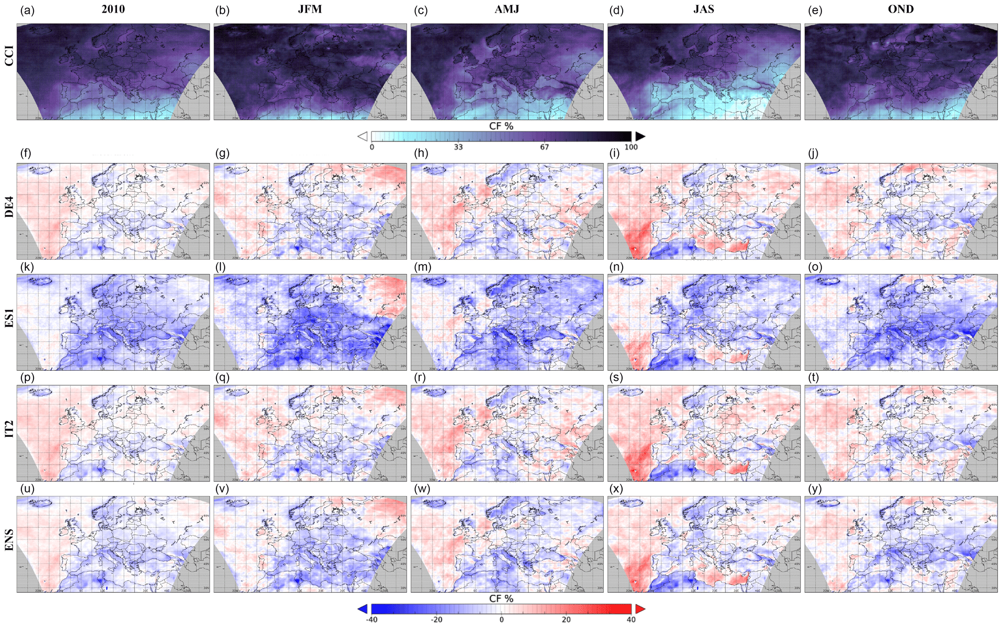
Figure 1Mean bias error (bias) CF. First row represents the mean satellite values of 2010 (first column), JFM (second column), AMJ (third column), JAS (fourth column), OND (fifth column). Following rows represent the bias of the models: DE4 – second row; ES1 – third row; IT2 – fourth row; NL2 – fifth row; UK4 – sixth row; ENS – seventh row.
2.3 Evaluation methodology
Regarding the model evaluation methodology, satellite data are bilinearly interpolated to a common working grid covering the European domain. For the evaluation of cloud variables, model data were post-processed by computing the monthly mean of the mean value from 13:00 to 14:00. In order to evaluate the studied variables, several classic statistics were used according to Willmott et al. (1985) and Weil et al. (1992). We computed the mean bias error (bias) and the correlation coefficient. The computation of the median showed identical spatial patterns, so only the mean results are shown.
The bias (Eq. 1) is defined as
where ei is the individual model-prediction errors usually defined as prediction (Pi) minus observations (Oi) and and are the model-predicted and observed means, respectively.
The standard deviation of the Pi (Eq. 2) is
The standard deviation of the Oi (Eq. 3) is
The correlation (Eq. 4) is
The standard deviation ratio was computed as σp∕σo. A satellite data mask for each monthly mean was done and applied to model data in order to compute the statistics over the same area. The mean values were computed and are discussed in Sect. 3. Since satellite data availability was monthly means, the temporal coefficient of correlation is only shown for the whole year (2010). To compute the correlation, a satellite data mask containing 6 months or more of satellite data was considered so that the correlation is shown only in the grid points where there are at least 6 months of data.
This section describes the behaviour of the studied variables (CF, IWP, LWP, COD) for the bias, temporal correlation, and spatial variability. They were obtained by calculating the corresponding statistics of the monthly mean series at each grid point of all the land grid points of the domain for each season as follows: January–February–March (JFM); April–May–June (AMJ); July–August–September (JAS); October–November–December (OND). The continental European domain includes the north of Africa, the western part of Russia, and Iceland. All the figures in the present study have the same structure (but temporal correlation). The top row represents the mean satellite values from ESA Cloud_cci (discontinuity features seen around 60∘ N are due to small inconsistencies between day, twilight, and night-time retrievals, which are found to be most prominent in regions with day and night-time observations bordering on regions without any daytime observations). From left to right, the mean for the analysed periods – 2010, JFM, AMJ, JAS, and OND – are depicted. The following rows (2 to 7) include the computed statistic for each model and the ensemble (ENS) mean, estimated as the average of all the available model simulations. The yearly correlation is shown for the temporal correlation. The first row shows the mean satellite data for the cloud variables (one in each column) for 2010, while the following rows show the temporal correlation for each simulation.
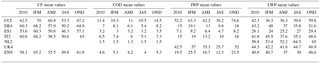
Table 2Mean satellite, model, and ensemble values for CF, COD, IWP, and LWP.
3.1 Cloud fraction, CF
Figure 1 shows the bias for the variable CF. In both cases, the first row shows the satellite CCI values, which are generally higher than 0, with minimum values over the eastern Mediterranean that increase with latitude. The values between 0 % and 1 % are found in some areas during summer months, mainly in northern Africa. The following rows show the bias of the different model simulations. Table 2 provides the mean values of satellite, models, and ENS. For CF, the mean model values come close to the satellite data, with a slight tendency for underestimation. Figure 1 generally indicates an underprediction for CF over land areas and an overestimation over the ocean. Individual model simulations present a bias range from +40 % to over −35 % over the studied region. The ES1 model presents the highest underestimation (−40 % mean bias), mainly over land areas. For the ENS mean (last row in Fig. 1), lower values are found, with biases ranging from 20 % to −20 %, which outperform the individual simulations. The positive bias is more marked during JAS, where the mean satellite values are lower (first row in Fig. 1). A negative bias is expected because of the general trend in global and regional models to underestimate CCN (Wyant et al., 2015) and, therefore, cloud formation. The overestimations found offshore could be produced because satellite retrievals missed thin clouds. Lastly, Fig. 2 represents the mean satellite data for the cloud variables in the first row for 2010. The following rows cover the temporal correlation for each model simulation. For CF, a positive temporal correlation prevails, with mean values of 0.7/0.8 and areas with values that come close to 0.9. Conversely, there are some areas over the sea with a negative correlation (around −0.5). This spatial pattern of the correlation coefficient is related to Fig. 1, where a negative bias prevails over land areas and a positive one over sea. Generally, a positive correlation implies that when the satellite CF values increase (decrease), the model's CF values increase (decrease) but models underestimate this mainly over land areas (Fig. 1).
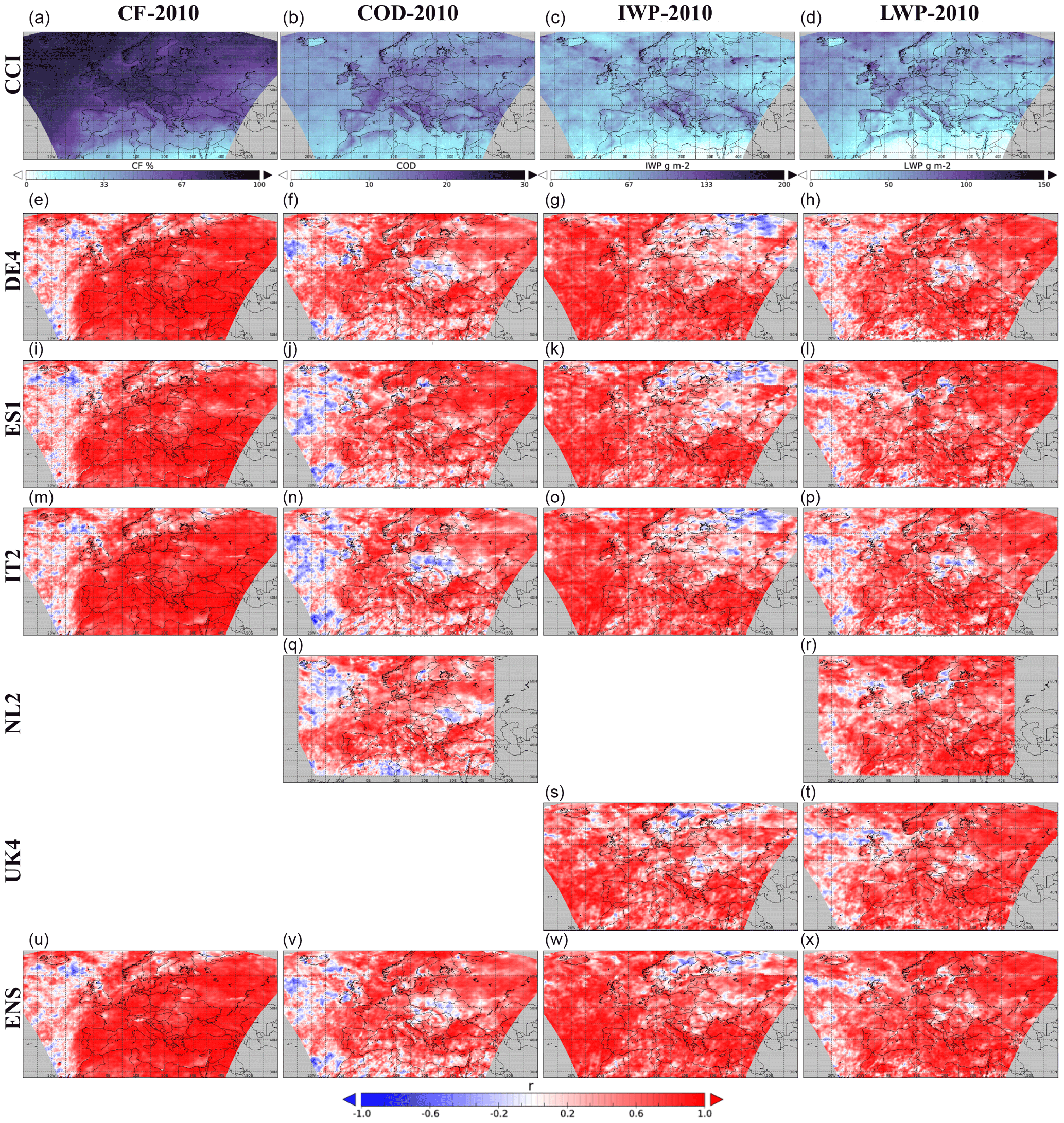
Figure 2Temporal correlation for the whole year 2010. First row represents the mean satellite values of 2010, where each column represents a cloud variable. The following rows show the temporal correlation of each model and cloud variable.
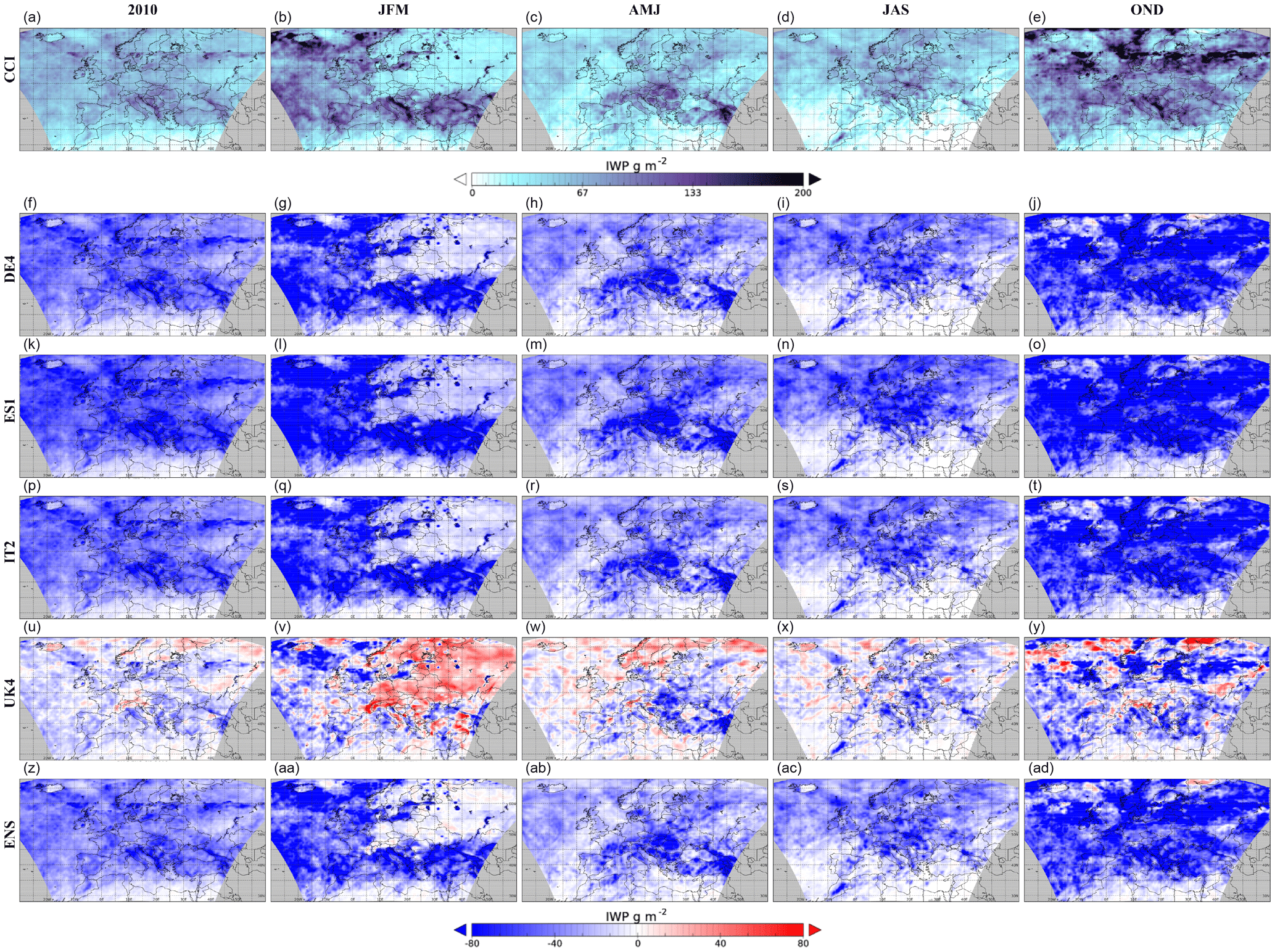
3.2 Cloud ice path, IWP
Regarding IWP, the all-sky mean was computed (also for the LWP variable). Figure 3 presents the mean satellite values (first row), where values below 100 g m−2 are mostly found. For some delimited areas, higher values are found (over 200 g m−2) during winter months (JFM, OND) and spring (AMJ). The third column in Table 2 reflects that the mean models values are significantly lower compared to the satellite retrievals for IWP. Therefore, the IWP bias in Fig. 3 shows a general model underestimation but for UK4. The WRF-Chem models (DE4, ES1, IT2) show negative biases between −80 and −50 g m−2 in different parts of the domain, depending on the season. The largest underestimations are found during JFM and OND (where the mean satellite values are very high). On the other hand, UK4 overestimates the IWP, with a positive bias of 80 g m−2 during JFM over central and northern Europe. During JFM, the mean satellite data were around 50 g m−2, which is best captured by the other models. UK4 also overestimates IWP for the rest of the year over some northern areas of the domain. The differences found here in relation to WRF-Chem models and UK4 could be related to the number of hydrometeors defined in each microphysics scheme. For both WRF-Chem microphysics (Lin et al., 1983; Morrison et al., 2009), three types of ice hydrometeors are considered, whereas UK4 considers only one (Wilson and Ballard, 1999). IWP is a prognostic variable in the UK4 model. The fact that the WRF-Chem simulations underestimate the IWP, with an overestimation in the UK4 model, could mean that the number of ice hydrometeors in the microphysics scheme is relevant for the IWP representation. At the same time, the ENS simulation outperforms the individual simulations because it compensates for the UK4 model overestimation by the underestimations of the other models. The temporal correlation (Fig. 2) shows positive correlation values around 0.7 and negative correlations between −0.5 and −0.6. Positive correlations are practically found in the entire domain, whereas negative correlations are found in northern Europe (Scandinavia and the north of Russia). Since the mean models values are significantly lower compared to the satellite retrievals and, together with the negative CCI bias against DARDAR, strengthens the conclusion that models have a very small IWP.
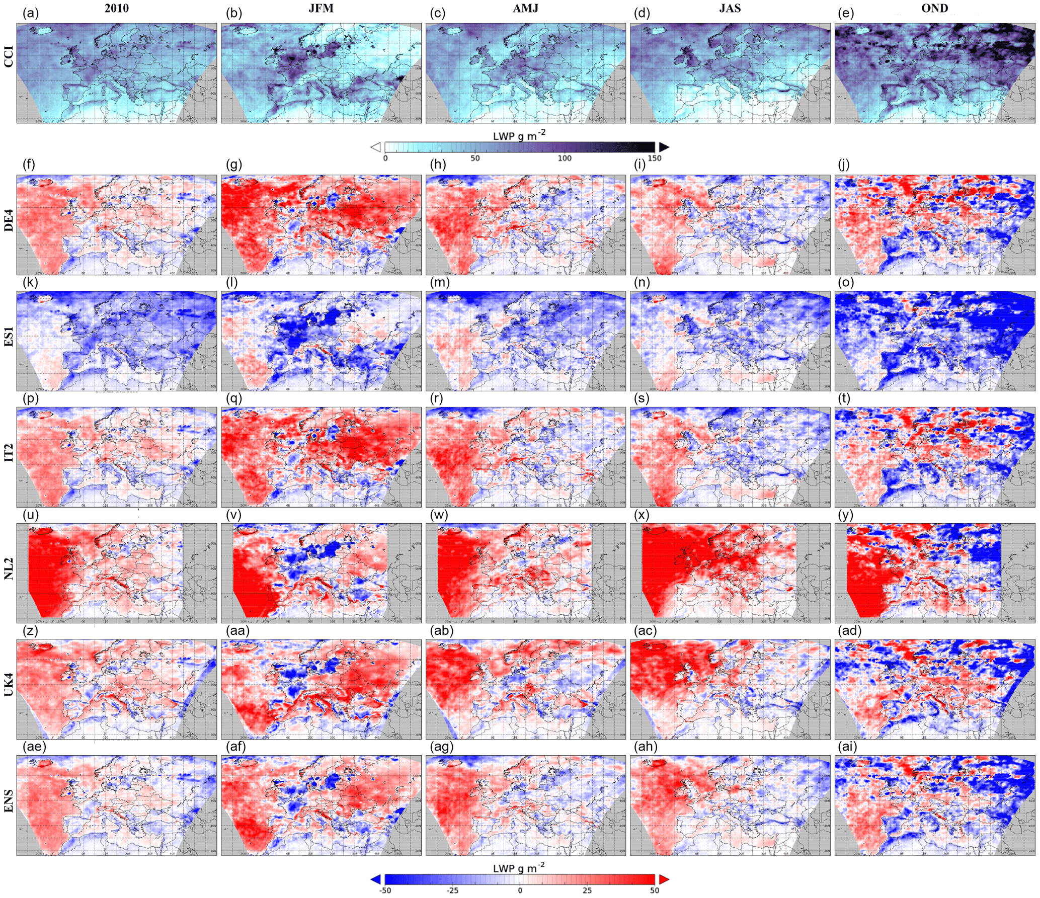
3.3 Cloud water path, LWP
The bias of the LWP is shown in Fig. 4. The mean satellite values (first row, Fig. 4) are below 100 g m−2 (as well as for IWP) but values are higher than 150 g m−2 in winter months (during JFM, mainly in the north of Spain, some areas of the Mediterranean coast, France, northern Europe, and the Baltic Sea; in OND). As for the IWP during OND, the LWP is higher over the entire domain (except for northern Africa). Greenwald et al. (1993) used the special sensor microwave/imager (SSM/I) to retrieve integrated LWP, which found values around 100 g m−2. Although the mean satellite data seem to be in agreement with other studies, the models shows higher LWP values. When the mean model values, except for the ES1 model (last column, Table 2), are higher compared to satellite values, we can see in Fig. 4 a general overestimation of the LWP (values of up to +50 g m−2), mainly over the sea. The model differences found here could be related to the LWP treatment in the model. For instance, in all the models except UK4, the LWP is treated as an prognostic variable whereas UK4 treats it as a diagnostic variable (Wilson and Ballard, 1999). Besides, within the WRF-Chem models and according to Baró et al. (2015), the models with a Morrison scheme have more droplets with a smaller diameter compared to the Lin scheme. This could also affect the representation of this variable, where the ES1 model underestimates the LWP over most of the domain. According to Tiedtke (1993), a correct representation of the LWP is important for high clouds because it is directly related to transparency or optical thickness. As will be shown in Sect. 3.4, NL2 underestimates COD (explained by the findings of Tompkins et al. (2007) when testing the scheme). No data are available to evaluate the IWP or LWP over northern Africa. The temporal correlation (Fig. 2) shows a positive correlation value of around 0.7 for most of the domain. Negative correlations prevail in the Atlantic Ocean and some parts of central Europe (up to −0.6).
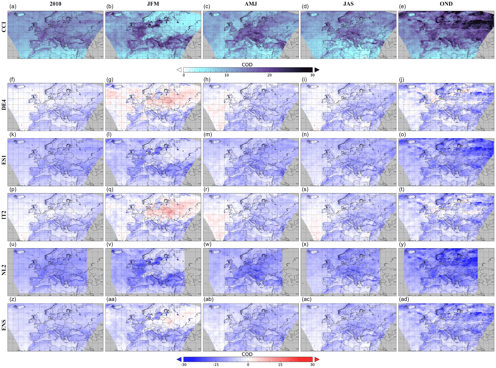
3.4 Cloud optical depth, COD
Regarding COD, the mean seasonal satellite values (first row in Fig. 5) go up to 30, with the highest mean values during the OND period. The lowest values are found over the northeastern part of the domain, with values under 10. The second column of Table 2 indicates that generally lower mean model values are found compared to the satellite data. This spatial pattern is clear in the COD bias (Fig. 5), with a general underestimation of the monthly mean COD over the whole domain.
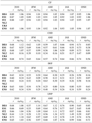
Table 3Spatial correlation and standard deviation ratio values for CF, COD, IWP, and LWP over the following periods: 2010, JFM, AMJ, JAS, OND. r: correlation coefficient; σP∕σO: ratio between the standard deviation of the models (σP) and the observations (σO).
In general, a higher negative bias is found during OND, and NL2 gives the largest underestimation (values of up to −30). In winter months (JFM), DE4 and IT2 show an overestimation over central Europe and some areas around +15, over the Atlantic Ocean, which coincide with the low COD values in the satellite. For the WRF-Chem models, the differences that appear between models can be related to the different microphysics scheme (Table 1) employed: Morrison (Morrison et al., 2009) in DE4 and IT2 and the Lin scheme (Lin et al., 1983) in ES1. According to Baró et al. (2015), who studied the differences between these microphysics schemes, Morrison parameterization involves higher droplet number mixing ratio values. Baró et al. (2015) stated that, since cloud water is similar for the Morrison and Lin simulations, the higher droplet number mixing ratio in Morrison indicates that cloud droplets have a smallers diameter in Morrison than in Lin (especially during winter). Since COD measures the attenuation of radiation due to extinction by cloud droplets, smaller and more cloud droplets in the Morrison scheme are more effective in scattering shortwave radiation and could explain the positive biases found in the DE4 and IT2 models. The differences found in the NL2 model may once again be related to its model microphysics scheme (Table 1) (Neggers, 2009; Tiedtke, 1993; Tompkins et al., 2007). Tompkins et al. (2007) tested the new scheme in the European Centre for Medium-Range Weather Forecasts (ECMWF), Integrated Forecasting System (IFS) model within two seven-member ensembles of 13 months. They made a comparison with the International Satellite Cloud Climatology Project (ISCCP) D2 retrievals and found a reduction in the high-cloud cover leading to a lower COD. This coincides with the results found herein, where this model presents the largest underestimations. Once again, the ENS simulation outperforms the individual simulations. Regarding the temporal correlation (second column in Fig. 2), a generally positive correlation is seen with values of up to 0.8 (mostly over land areas); others with a negative correlation are seen over central Europe in models DE4 and IT2, which coincides with those areas where the bias is overestimated.
3.5 Spatial correlation and variability
The spatial correlation and variability, averaged for year and target season, are summarized in Table 3 for each variable (CF, COD, IWP, and LWP, in that order). For the CF, the seasonal correlation coefficients are very high (over 0.90 for each model and season, except for ES1 in wintertime, with a correlation of 0.89). Yearly correlation coefficients range from 0.85 to 0.89, which indicates that the models are able to capture the spatial variability in the CF well. The σP∕σO ratio provides an idea of the trend in the simulations to overestimate or underestimate the spatial variability (ratio over or under 1, respectively). All the models present accurate spatial variability representativity, with ratios coming very close to 1 for every season and also for the annual average. All the models have a very slight tendency to overestimate CF spatial variability (the σP∕σO ratio ranging from 1.01 to 1.07).
The spatial correlation coefficient for the other variables indicates less capacity to represent the spatial correlation of COD, IWP, and LWP. All the annual spatial correlation values are in the order of 0.6–0.7 and range from the case of NL2 for COD (0.41) and LWP (0.44) at the bottom to the simulation of UK4 for the LWP (0.73). These values are similar if seasonal correlation coefficients are observed, except for summertime and the IWP variable. The model's capacity to represent the IWP spatial pattern is limited during JAS, with correlation coefficients ranging from 0.16 in UK4 to 0.35 in DE4 and IT2. Once again, the Morrison microphysics seems to outperform all the other simulations when representing the cloud ice path.
As for the spatial variability in COD, IWP, and LWP, represented by the σP∕σO ratio, major differences between the variables and models are found. For the COD, ES1 and NL2 tend to underestimate its spatial variability, especially for NL2, with σP∕σO values ranging from 0.09 during OND to 0.17 for summertime (JAS). The other models present a good capacity to reproduce variability, with slightly higher ratios for the yearly-averaged values than for individual seasons. For the IWP, spatial variability is generally estimated by all the models and seasons (σP∕σO values in the order of 0.1–0.2), except for UK4, which slightly underpredicts variability (ratios around 0.8, except for OND, when this value drops to 0.63).
Lastly, for the LWP, all the models but ES1 slightly overestimate the spatial variability (σP∕σO values around 1.0–1.3) for the yearly-averaged values in winter and spring. In summer, this value is slightly overestimated by the simulations that do not use WRF-Chem (around 1.4 for NL2 and 1.2 for UK4), while for autumn (OND) all the models tend to underpredict the spatial variability (values of 0.7/0.8). In general, the best capacities are found for the DE4 simulations, while the largest underestimations are present in the ES1 simulations, which use the Lin microphysics scheme, with values around 0.6.
The presence or the absence of cloudiness must be well represented in modelling since clouds play an important role in the Earth's energy balance (Boucher et al., 2013; Myhre et al., 2013). Hence, a collective evaluation of the cloud variables CF, COD, IWP, and LWP is shown in this study. The simulations evaluated herein were run by coupled chemistry and meteorology models in the AQMEII Phase 2 initiative context for the year 2010. This study complements other collective analyses, such as Baró et al. (2017), Brunner et al. (2015), Makar et al. (2015a), Makar et al. (2015b), and Forkel et al. (2015) by adding an assessment of how online-coupled models represent some cloud properties in an ensemble of simulations.
As for the CF, an underestimation (overestimation) of this variable is observed over land (sea) areas. Individual model simulations present a positive bias close to 40 % and a negative bias over −35 %. For the ensemble mean, lower CF values are found, with biases ranging from 20 % to −20 %, which outperform individual simulations. The positive bias is more pronounced during JAS, where the mean satellite values are lower. The negative bias may be due to the general underestimation in the CCN representation by global and regional models (Wyant et al., 2015). The overestimations found offshore might be related to satellite retrievals missing thin clouds. A positive temporal coefficient of correlation dominates in the spatial pattern of CF (values close to 0.9) and a negative correlation (around −0.5) in some areas over the sea. This is similar to the bias, where a negative bias prevailed over land areas and a positive bias over the sea.
There is an overall underestimation of the IWP, except in UK4. The differences found here in relation to the WRF-Chem models and UK4 could be related to the number of hydrometeors defined in each microphysics scheme. For both WRF-Chem microphysics, three types of ice hydrometeors are considered, whereas UK4 (Wilson and Ballard, 1999) considers only one. So the overestimation found in the UK4 model could mean that the number of ice hydrometeors is relevant. The temporal correlation shows positive correlation values at around 0.7 and negative correlations between −0.5 and −0.6. A positive correlation is found over nearly the whole target domain, whereas negative correlations are found in northern Europe (Scandinavian countries and the north of Russia).
Despite the LWP mean satellite data seeming to be in agreement with other studies (Kniffka et al., 2014), models shows higher LWP values that result in a general LWP overestimation, mainly over sea areas (except the ES1 model). The model differences found here could be related to the treatment of the variable because, for instance, in all the models except for UK4, LWP is treated as an prognostic variable, whereas UK4 treats it as a diagnostic variable (Wilson and Ballard, 1999). As seen in Sect. 3.4, in the WRF-Chem models and according to Baró et al. (2015), the models with the Morrison scheme have more droplets with a smaller diameter compared to the Lin scheme. This could also affect the representation of this variable by showing an ES1 model underestimation over most of the domain. According to Tiedtke (1993), a correct representation of the LWP is important for high clouds, given its directly relation to transparency or optical thickness. Besides, as mentioned in Sect. 3.4, NL2 underestimates COD. The temporal correlation shows positive values at around 0.7 for most of the domain. Negative correlations prevail in the Atlantic Ocean and some parts of central Europe (up to −0.6).
Regarding COD, lower mean model values are found compared to the satellite data, resulting in a general underestimation of the monthly mean over the whole domain. A generally higher negative bias is found during OND, with NL2 showing the largest underestimation. In winter, DE4 and IT2 tend to overestimate over central Europe and some areas over the Atlantic Ocean, which corresponds to low COD values, as indicated by the satellite. These differences in the WRF-Chem models may be related to the different microphysics scheme used (Morrison (Morrison et al., 2009) versus Lin (Lin et al., 1983)). In the former, cloud droplets have a smaller diameter than Lin (especially during winter) (Baró et al., 2015), which leads to more effective extinction by cloud droplets. The differences found in the NL2 model may be related to the model microphysics scheme. Temporal correlation indicates a generally positive correlation between models and satellite observations, with values of up to 0.8 (mostly over land areas). Some areas with a negative correlation over central Europe in models DE4 and IT2 are related to areas with an overestimation trend.
Finally, the seasonal and yearly correlation coefficients are very high for the CF (seasonal over 0.90, yearly over 0.85), which indicates that the models are able to capture the spatial variability well, while they tend to slightly overestimate CF spatial variability (σP∕σO values ranging from 1.01 to 1.07). The other variables indicate less capacity to represent the spatial correlation of the COD, IWP, and LWP. All the annual spatial correlation values are in the order of 0.6–0.7, which are similar when seasonal correlation coefficients are observed, except for the IWP in the summertime. The models' capacity to represent the IWP spatial pattern is limited during JAS (correlation coefficients ranging from 0.16 to 0.35). Morrison microphysics seems to outperform the other simulations when representing the cloud ice path. Major differences in the spatial variability between the variables and models are found. For COD, ES1 and NL2 tend to underestimate their spatial variability, especially for NL2, with σP∕σO values ranging from 0.09 during OND to 0.17 for the summertime (JAS). The other models present a good capacity to reproduce the variability, with slightly higher ratios for the yearly-averaged values. With the IWP, the spatial variability is pervasively estimated by all the models and seasons, except for UK4, which slightly underpredicts the variability (with ratios around 0.8, except for OND, when this value drops to 0.63). For the LWP, all the models but ES1 slightly overestimate the spatial variability (σP∕σO values around 1.0–1.3) for the yearly-averaged values, winter, and spring. In summer, the best capacities go to the DE4 simulations, while the largest underestimations are present for ES1 simulations (which use Lin microphysics scheme).
According to Rosenfeld et al. (2014), a better understanding of the aerosol–cloud processes would reduce the uncertainty in anthropogenic climate forcing and provide a clear understanding and better predictions of the future impacts of aerosols on both climate and weather. With this study, it has been shown how the online coupled models represent several cloud properties, which complements the temperature collective analyses of Baró et al. (2017).
Data are accessible by contacting the corresponding author (pedro.jimenezguerrero@um.es) or the authors from each institution for individual model simulations. Satellite data are available through the ESA – Climate Change Initiative (CCI) Open Portal (http://cci.esa.int/data, last access: January 2017).
RB, PJG, and LPP carried out the ES1 simulations and analyses of the data from all groups; RB prepared the manuscript with contributions from all co-authors; DB helped in the design of the study and contacted MSt, who provided the Cloud_cci data used in this study; GC and PT carried out the IT2 simulations; RF carried out the DE4 simulations; LN and NS carried out the UK4 simulations; MSc and HDvdG carried out the NL2 simulations. SG coordinated and designed the experimental setup of the AQMEII3 exercise.
The authors declare that they have no conflict of interest.
This article is part of the special issue “Global and regional assessment of intercontinental transport of air pollution: results from HTAP, AQMEII and MICS”. It is not associated with a conference.
Special acknowledgment is due to the ESA CCI Cloud team, who provided us with the Cloud
data for doing this study. We also acknowledge the initiative AQMEII2 and the
Joint Research Center Ispra and the Institute for Environment and
Sustainability for its ENSEMBLE system. The group from University of L'Aquila
kindly thanks the EuroMediterranean Centre on Climate Change (CMCC) for the
computational resources. Paolo Tuccella is a beneficiary of an AXA Research Fund
postdoctoral grant. The Project ACEX (CGL2017-87921-R), funded by the Spanish
Ministerio de Economía y Competitividad (MINECO) and the FEDER European
program, has supported the completion of this study. The author Rocío
Baró acknowledges the FPU scholarship (ref. FPU12/05642) by the Spanish
Ministerio de Educación, Cultura y Deporte. Pedro Jiménez-Guerrero
acknowledges the fellowship 19677/EE/14 of the Programme Jiménez de la Espada de Movilidad, Cooperación e Internacionalización (Fundación
Séneca-Agencia de Ciencia y Tecnología de la Región de Murcia, PCTIRM
2011–2014).
Edited by: Johannes Quaas
Reviewed by: two anonymous referees
Alapaty, K., Mathur, R., Pleim, J., Hogrefe, C., Rao, S. T., Ramaswamy, V., Galmarini, S., Schaap, M., Makar, P., Vautard, R., Makar, P., Baklanov, A., Kallos, G., Vogel , B., Hogrefe, C., and Sokhi, R.: New Directions: Understanding interactions of air quality and climate change at regional scales, Atmos. Environ., 49, 419–421, 2012.
Albrecht, B. A.: Aerosols, cloud microphysics, and fractional cloudiness, Science, 245, 1227–1230, 1989. a
Avey, L., Garrett, T. J., and Stohl, A.: Evaluation of the aerosol indirect effect using satellite, tracer transport model, and aircraft data from the International Consortium for Atmospheric Research on Transport and Transformation, J. Geophys. Res.-Atmos., 112, https://doi.org/10.1029/2006JD007581, 2007. a
Baklanov, A., Korsholm, U., Woetmann, N., and Gross, A.: On-line coupling of chemistry and aerosols into meteorological models: advantages and prospective, Tech. rep., Project no. 516099, Danish Meteorological Institute (DMI), Copenhagen, 2008. a
Baró, R., Jiménez-Guerrero, P., Balzarini, A., Curci, G., Forkel, R., Grell, G., Hirtl, M., Honzak, L., Langer, M., Pérez, J. L., Pirovano, G., San José, R., Tuccella, P., Werhahn, J., and Zabkar, R.: Sensitivity analysis of the microphysics scheme in WRF-Chem contributions to AQMEII phase 2, Atmos. Environ., 115, 620–629, 2015. a, b, c, d, e
Baró, R., Palacios-Peña, L., Baklanov, A., Balzarini, A., Brunner, D., Forkel, R., Hirtl, M., Honzak, L., Pérez, J. L., Pirovano, G., San José, R., Schröder, W., Werhahn, J., Wolke, R., Žabkar, R., and Jiménez-Guerrero, P.: Regional effects of atmospheric aerosols on temperature: an evaluation of an ensemble of online coupled models, Atmos. Chem. Phys., 17, 9677–9696, https://doi.org/10.5194/acp-17-9677-2017, 2017. a, b
Baum, B. A., Yang, P., Heymsfield, A. J., Schmitt, C. G., Xie,Y., Bansemer, A., Hu, Y. X., and Zhang, Z.: Improvements in Shortwave Bulk Scattering and Absorption Models for the Remote Sensing of Ice Clouds, J. Appl. Meteorol., 50, 1037–1056, 2011. a
Baum, B. A., Yang, P., Heymsfield, A. J., Bansemer, A., Cole, B. H., Merrelli, A., Schmitt, C., and Wang, C.: Ice Cloud Single-Scattering Property Models with the Full Phase Matrix at Wave-lengths from 0.2 to 100 µm, J. Quant. Spectrosc. Ra., 146, 123–139, 2014. a
Boucher, O.: Atmospheric Aerosols: Properties and Climate Impacts, Springer, 2015.
Boucher, O. and Lohmann, U.: The sulfate-CCN-cloud albedo effect, Tellus B, 47, 281–300, 1995. a
Boucher, O., Randall, D., Artaxo, P., Bretherton, C., Feingold, G., Forster, P., Kerminen, V.-M., Kondo, Y., Liao, H., Lohmann, U., Rash, P., Satheesh, S., Sherwood, S., Stevens, B., and Zhang, X.-Y.: Clouds and Aerosols. In: Climate Change 2013: The Physical Science Basis. Contribution of Working Group I to the Fifth Assessment Report of the Intergovernmental Panel on Climate Change, Cambridge University Press, Cambridge, United Kingdom and New York, USA, 2013. a, b
Brunner, D., Savage, N., Jorba, O., Eder, B., Giordano, L., Badia, A., Balzarini, A., Baró, R., Bianconi, R., Chemel, C., Curci, G., Forkel, R., Jiménez-Guerrero, P., Hirtl, M., Hodzic, A., Honzak, L., Im, U., Knote, C., Makar, P., Manders-Groot, A., van Meijgaard, E., Neal, L., Pérez, J. L., Pirovano, G., José, R. S., Schroder, W., Sokhi, R. S., Syrakov, D., Torian, A., Tuccella, P., Werhahn, J., Wolke, R., Yahya, K., Zabkar, R., Zhang, Y., Hogrefe, C., and Galmarini, S.: Comparative analysis of meteorological performance of coupled chemistry-meteorology models in the context of AQMEII phase 2, Atmos. Environ., 115, 470–498, 2015. a, b, c
Curry, J. A., Ardeel, C. D., and Tian, L.: Liquid water content and precipitation characteristics of stratiform clouds as inferred from satellite microwave measurements, J. Geophys. Res.-Atmos., 95, 16659–16671, 1990.
Delanoë, J. and Hogan, R. J.: A variational scheme for retrieving ice cloud properties from combined radar, lidar, and infrared radiometer, J. Geophys. Res., 113, D07204, https://doi.org/10.1029/2007JD009000, 2008. a
Delanoë, J. and Hogan, R. J.: Combined CloudSat–CALIPSO–MODIS retrievals of the properties of ice clouds, J. Geophys. Res., 115, D00H29, https://doi.org/10.1029/2009JD012346, 2010. a
Forkel, R., Balzarini, A., Baró, R., Bianconi, R., Curci, G., Jiménez-Guerrero, P., Hirtl, M., Honzak, L., Lorenz, C., Im, U., Pérez, J. L., Pirovano, G., José, R. S., Tuccella, P., Werhahn, J., and Zabkar, R.: Analysis of the WRF-Chem contributions to AQMEII phase2 with respect to aerosol radiative feedbacks on meteorology and pollutant distributions, Atmos. Environ., 115, 630–645, 2015. a
Galmarini, S., Hogrefe, C., Brunner, D., Makar, P., and Baklanov, A.: Preface, Atmos. Environ., 115, 340–344, 2015.
Grainger, R. G., Lucas, J., Thomas, G. E., and Ewen, G. B. L.: Calculation of Mie derivatives, Appl. Optics, 43, 5386–5393, 2004. a
Greenwald, T. J., Stephens, G. L., Vonder Haar, T. H., and Jackson, D. L.: A physical retrieval of cloud liquid water over the global oceans using special sensor microwave/imager (SSM/I) observations, J. Geophys. Res., 98, 18471–18488, 1993. a
Grell, G. and Baklanov, A.: Integrated modeling for forecasting weather and air quality: A call for fully coupled approaches, Atmos. Environ., 45, 6845–6851, 2011. a
Grell, G. A., Peckham, S. E., Schmitz, R., McKeen, S. A., Frost, G., Skamarock, W. C., and Eder, B.: Fully coupled “online” chemistry within the WRF model, Atmos. Environ., 39, 6957–6975, 2005. a
Guenther, A., Karl, T., Harley, P., Wiedinmyer, C., Palmer, P. I., and Geron, C.: Estimates of global terrestrial isoprene emissions using MEGAN (Model of Emissions of Gases and Aerosols from Nature), Atmos. Chem. Phys., 6, 3181–3210, https://doi.org/10.5194/acp-6-3181-2006, 2006. a
Hollmann, R., Merchant, C., Saunders, R., Downy, C., Buchwitz, M., Cazenave, A., Chuvieco, E., Defourny, P., de Leeuw, G., Forsberg, R., Holzer-Popp, T., Paul, F., Sandven, S., Sathyendranath, S., Van Roozendael, M., and W, W.: The ESA climate change initiative: Satellite data records for essential climate variables, B. Am. Meteorol. Soc., 94, 1541–1552, 2013. a
Im, U., Bianconi, R., Solazzo, E., Kioutsioukis, I., Badia, A., Balzarini, A., Baró, R., Bellasio, R., Brunner, D., Chemel, C., Curci, G., Flemming, J., Forkel, R., Giordano, L., Jiménez-Guerrero, P., Hirtl, M., Hodzic, A., Honzak, L., Jorba, O., Knote, C., Kuenen, J. J., Makar, P. A., Manders-Groot, A., Neal, L., Pérez, J. L., Pirovano, G., Pouliot, G., Jose, R. S., Savage, N., Schroder, W., Sokhi, R. S., Syrakov, D., Torian, A., Tuccella, P., Werhahn, J., Wolke, R., Yahya, K., Zabkar, R., Zhang, Y., Zhang, J., Hogrefe, C., and Galmarini, S.: Evaluation of operational on-line-coupled regional air quality models over Europe and North America in the context of AQMEII phase 2. Part I: Ozone, Atmos. Environ., 115, 404–420, 2015a. a, b
Im, U., Bianconi, R., Solazzo, E., Kioutsioukis, I., Badia, A., Balzarini, A., Baró, R., Bellasio, R., Brunner, D., Chemel, C., Curci, G., van der Gon, H. D., Flemming, J., Forkel, R., Giordano, L., Jiménez-Guerrero, P., Hirtl, M., Hodzic, A., Honzak, L., Jorba, O., Knote, C., Makar, P. A., Manders-Groot, A., Neal, L., Pérez, J. L., Pirovano, G., Pouliot, G., Jose, R. S., Savage, N., Schroder, W., Sokhi, R. S., Syrakov, D., Torian, A., Tuccella, P., Wang, K., Werhahn, J., Wolke, R., Zabkar, R., Zhang, Y., Zhang, J., Hogrefe, C., and Galmarini, S.: Evaluation of operational online-coupled regional air quality models over Europe and North America in the context of AQMEII phase 2. Part II: Particulate matter, Atmos. Environ., 115, 421–441, 2015b. a, b
Janssens-Maenhout, G., Crippa, M., Guizzardi, D., Dentener, F., Muntean, M., Pouliot, G., Keating, T., Zhang, Q., Kurokawa, J., Wankmüller, R., Denier van der Gon, H., Kuenen, J. J. P., Klimont, Z., Frost, G., Darras, S., Koffi, B., and Li, M.: HTAP_v2.2: a mosaic of regional and global emission grid maps for 2008 and 2010 to study hemispheric transport of air pollution, Atmos. Chem. Phys., 15, 11411–11432, https://doi.org/10.5194/acp-15-11411-2015, 2015. a
Kniffka, A., Stengel, M., Lockhoff, M., Bennartz, R., and Hollmann, R.: Characteristics of cloud liquid water path from SEVIRI onboard the Meteosat Second Generation 2 satellite for several cloud types, Atmos. Meas. Tech., 7, 887–905, https://doi.org/10.5194/amt-7-887-2014, 2014. a
Lin, Y. L., Farley, R. D., and Orville, H. D.: Bulk parameterization of the snow field in a cloud model, J. Clim. Appl. Meteorol., 22, 1065–1092, 1983. a, b, c
Liu, Y., Wu, W., Jensen, M. P., and Toto, T.: Relationship between cloud radiative forcing, cloud fraction and cloud albedo, and new surface-based approach for determining cloud albedo, Atmos. Chem. Phys., 11, 7155–7170, https://doi.org/10.5194/acp-11-7155-2011, 2011. a
Lohmann, U. and Feichter, J.: Global indirect aerosol effects: a review, Atmos. Chem. Phys., 5, 715–737, https://doi.org/10.5194/acp-5-715-2005, 2005. a
Makar, P., Gong, W., Milbrandt, J., Hogrefe, C., Zhang, Y., Curci, G., Zabkar, R., Im, U., Balzarini, A., Baró, R., Bianconi, R., Cheung, P., Forkel, R., Gravel, S., Hirtl, M., Honzak, L., Hou, A., Jiménez-Guerrero, P., Langer, M., Moran, M., Pabla, B., Pérez, J., Pirovano, G., José, R. S., Tuccella, P., Werhahn, J., Zhang, J., and Galmarini, S.: Feedbacks between air pollution and weather, Part 1: Effects on weather, Atmos. Environ., 115, 442–469, 2015a. a, b
Makar, P., Gong, W., Hogrefe, C., Zhang, Y., Curci, G., Zabkar, R., Milbrandt, J., Im, U., Balzarini, A., Baró, R., Bianconi, R., Cheung, P., Forkel, R., Gravel, S., Hirtl, M., Honzak, L., Hou, A., Jiménez-Guerrero, P., Langer, M., Moran, M., Pabla, B., Pérez, J., Pirovano, G., José, R. S., Tuccella, P., Werhahn, J., Zhang, J., and Galmarini, S.: Feedbacks between air pollution and weather, part 2: effects on chemistry, Atmos. Environ., 115, 499–526, 2015b. a
McComiskey, A., Feingold, G., Frisch, A. S., Turner, D. D., Miller, M. A., Chiu, J. C., Min, Q., and Ogren, J. A.: An assessment of aerosol-cloud interactions in marine stratus clouds based on surface remote sensing, J. Geophys. Res.-Atmos., 114, https://doi.org/10.1029/2008JD011006, 2009. a
McGarragh, G. R., Poulsen, C. A., Thomas, G. E., Povey, A. C., Sus, O., Stapelberg, S., Schlundt, C., Proud, S., Christensen, M. W., Stengel, M., Hollmann, R., and Grainger, R. G.: The Community Cloud retrieval for CLimate (CC4CL) – Part 2: The optimal estimation approach, Atmos. Meas. Tech., 11, 3397–3431, https://doi.org/10.5194/amt-11-3397-2018, 2018. a, b
Menon, S., Genio, A. D. D., Koch, D., and Tselioudis, G.: GCM simulations of the aerosol indirect effect: Sensitivity to cloud parameterization and aerosol burden, J. Atmos. Sci., 59, 692–713, 2002.
Morrison, H., Thompson, G., and Tatarskii, V.: Impact of cloud microphysics on the development of trailing stratiform precipitation in a simulated squall line: Comparison of one-and two-moment schemes, Mon. Weather Rev., 137, 991–1007, 2009. a, b, c
Myhre, G., Shindell, D., Breon, F.-M., Collins, W., Fuglestvedt, J., Huang, J., Koch, D., Lamarque, J.-F., Lee, D., Mendoza, B., Nakajima, T., Robock, A., Stephens, G., Takemura, T., and H, Z.: Anthropogenic and Natural Radiative Forcing, in: Climate Change 2013: The Physical Science Basis, Contribution of Working Group I to the Fifth Assessment Report of the Intergovernmental Panel on Climate Change, Cambridge University Press, Cambridge, United Kingdom and New York, USA, 2013. a, b
Neggers, R. A.: A dual mass flux framework for boundary layer convection. Part II: Clouds, J. Atmos. Sci., 66, 1489–1506, 2009. a
Penner, J. E., Quaas, J., Storelvmo, T., Takemura, T., Boucher, O., Guo, H., Kirkevåg, A., Kristjánsson, J. E., and Seland, Ø.: Model intercomparison of indirect aerosol effects, Atmos. Chem. Phys., 6, 3391–3405, https://doi.org/10.5194/acp-6-3391-2006, 2006. a
Pouliot, G., Pierce, T., Denier van der Gon, H., Schaap, M., Moran, M., and Nopmongcol, U.: Comparing emission inventories and model-ready emission datasets between Europe and North America for the AQMEII project, Atmos. Environ., 53, 4–14, 2012. a
Quaas, J., Ming, Y., Menon, S., Takemura, T., Wang, M., Penner, J. E., Gettelman, A., Lohmann, U., Bellouin, N., Boucher, O., Sayer, A. M., Thomas, G. E., McComiskey, A., Feingold, G., Hoose, C., Kristjánsson, J. E., Liu, X., Balkanski, Y., Donner, L. J., Ginoux, P. A., Stier, P., Grandey, B., Feichter, J., Sednev, I., Bauer, S. E., Koch, D., Grainger, R. G., Kirkevåg, A., Iversen, T., Seland, Ø., Easter, R., Ghan, S. J., Rasch, P. J., Morrison, H., Lamarque, J.-F., Iacono, M. J., Kinne, S., and Schulz, M.: Aerosol indirect effects – general circulation model intercomparison and evaluation with satellite data, Atmos. Chem. Phys., 9, 8697–8717, https://doi.org/10.5194/acp-9-8697-2009, 2009. a
Rao, S. T., Galmarini, S., and Puckett, K.: Air Quality Model Evaluation International Initiative (AQMEII): advancing the state of the science in regional photochemical modeling and its applications, B. Am. Meteorol. Soc., 92, 23–30, 2011. a
Rosenfeld, D., Sherwood, S., Wood, R., and Donner, L.: Climate Effects of Aerosol-Cloud Interactions, Science, 343, 379–380, https://doi.org/10.1126/science.1247490, 2014. a, b
Sauter, F., van der Swaluw, E., Manders-Groot, A., Kruit, R. W., Segers, A., and Eskes, H.: LOTOS-EUROS v1.8 Reference Guide, TNO report TNO-060-UT-2012-01451, TNO, 2012. a
Savage, N. H., Agnew, P., Davis, L. S., Ordóñez, C., Thorpe, R., Johnson, C. E., O'Connor, F. M., and Dalvi, M.: Air quality modelling using the Met Office Unified Model (AQUM OS24-26): model description and initial evaluation, Geosci. Model Dev., 6, 353–372, https://doi.org/10.5194/gmd-6-353-2013, 2013. a
Schwartz, S. E. and Benkovitz, C. M.: Influence of anthropogenic aerosol on cloud optical depth and albedo shown by satellite measurements and chemical transport modeling, P. Natl. Acad. Sci., 99, 1784–1789, 2002. a
Seinfeld, J. H., Bretherton, C., Carslaw, K. S., Coe, H., DeMott, P. J., Dunlea, E. J., Feingold, G., Ghan, S., Guenther, A. B., Kahn, R., Kraucunas, I., Kreidenweis, S. M., Molina, M. J., Nenes, A., Penner, J. E., Prather, K. A., Ramanathan, V., Ramaswamy, V., Rasch, P. J., Ravishankara, A. R., Rosenfeld, D., Stephens, G., and Wood, R.: Improving our fundamental understanding of the role of aerosol–cloud interactions in the climate system, P. Natl. Acad. Sci., 113, 5781–5790, 2016.
Shindell, D. T., Lamarque, J.-F., Schulz, M., Flanner, M., Jiao, C., Chin, M., Young, P. J., Lee, Y. H., Rotstayn, L., Mahowald, N., Milly, G., Faluvegi, G., Balkanski, Y., Collins, W. J., Conley, A. J., Dalsoren, S., Easter, R., Ghan, S., Horowitz, L., Liu, X., Myhre, G., Nagashima, T., Naik, V., Rumbold, S. T., Skeie, R., Sudo, K., Szopa, S., Takemura, T., Voulgarakis, A., Yoon, J.-H., and Lo, F.: Radiative forcing in the ACCMIP historical and future climate simulations, Atmos. Chem. Phys., 13, 2939–2974, https://doi.org/10.5194/acp-13-2939-2013, 2013.
Solazzo, E. and Galmarini, S.: Error apportionment for atmospheric chemistry-transport models – a new approach to model evaluation, Atmos. Chem. Phys., 16, 6263–6283, https://doi.org/10.5194/acp-16-6263-2016, 2016.
Stengel, M., Stapelberg, S., Sus, O., Schlundt, C., Poulsen, C., Thomas, G., Christensen, M., Carbajal Henken, C., Preusker, R., Fischer, J., Devasthale, A., Willén, U., Karlsson, K.-G., McGarragh, G. R., Proud, S., Povey, A. C., Grainger, R. G., Meirink, J. F., Feofilov, A., Bennartz, R., Bojanowski, J. S., and Hollmann, R.: Cloud property datasets retrieved from AVHRR, MODIS, AATSR and MERIS in the framework of the Cloud_cci project, Earth Syst. Sci. Data, 9, 881–904, https://doi.org/10.5194/essd-9-881-2017, 2017a. a, b, c
Stengel, M., Sus, O., Stapelberg, S., Schlundt, C., Poulsen, C., and Hollmann, R.: ESA Cloud Climate Change Initiative (ESA Cloud_cci) data: Cloud_cci AVHRR–PM L3C/L3U CLD_PRODUCTS v2.0, Deutscher Wetterdienst (DWD), https://doi.org/10.5676/DWD/ESA_Cloud_cci/AVHRR-PM/V002, 2017b. a
Stevens, B. and Feingold, G.: Untangling aerosol effects on clouds and precipitation in a buffered system, Nature, 461, 607–613, 2009.
Sus, O., Stengel, M., Stapelberg, S., McGarragh, G., Poulsen, C., Povey, A. C., Schlundt, C., Thomas, G., Christensen, M., Proud, S., Jerg, M., Grainger, R., and Hollmann, R.: The Community Cloud retrieval for CLimate (CC4CL) – Part 1: A framework applied to multiple satellite imaging sensors, Atmos. Meas. Tech., 11, 3373–3396, https://doi.org/10.5194/amt-11-3373-2018, 2018. a
Taylor, K. E.: Summarizing multiple aspects of model performance in a single diagram, J. Geophys. Res.-Atmos., 106, 7183–7192, 2001.
Tiedtke, M.: Representation of clouds in large-scale models, Mon. Weather Rev., 121, 3040–3061, 1993. a, b, c
Tompkins, A. M., Gierens, K., and Rädel, G.: Ice supersaturation in the ECMWF integrated forecast system, Q. J. Roy. Meteorol. Soc., 133, 53–63, 2007. a, b, c
Twomey, S.: Pollution and the planetary albedo, Atmos. Environ., 8, 1251–1256, 1974. a
Twomey, S.: The influence of pollution on the shortwave albedo of clouds, J. Atmos. Sci., 34, 1149–1152, 1977. a
Weil, J., Sykes, R., and Venkatram, A.: Evaluating air-quality models: review and outlook, J. Appl. Meteorol., 31, 1121–1145, 1992. a
Willmott, C. J., Ackleson, S. G., Davis, R. E., Feddema, J. J., Klink, K. M., Legates, D. R., O'Donnell, J., and Rowe, C. M.: Statistics for the evaluation and comparison of models, J. Geophys. Res., 90, 8995–9005, 1985. a
Wilson, D. R. and Ballard, S. P.: A microphysically based precipitation scheme for the UK Meteorological Office Unified Model, Q. J. Roy. Meteorol. Soc., 125, 1607–1636, 1999. a, b, c, d
Wyant, M. C., Bretherton, C. S., Wood, R., Carmichael, G. R., Clarke, A., Fast, J., George, R., Gustafson Jr., W. I., Hannay, C., Lauer, A., Lin, Y., Morcrette, J.-J., Mulcahy, J., Saide, P. E., Spak, S. N., and Yang, Q.: Global and regional modeling of clouds and aerosols in the marine boundary layer during VOCALS: the VOCA intercomparison, Atmos. Chem. Phys., 15, 153–172, https://doi.org/10.5194/acp-15-153-2015, 2015. a, b
Yang, Q., W. I. Gustafson Jr., Fast, J. D., Wang, H., Easter, R. C., Morrison, H., Lee, Y.-N., Chapman, E. G., Spak, S. N., and Mena-Carrasco, M. A.: Assessing regional scale predictions of aerosols, marine stratocumulus, and their interactions during VOCALS-REx using WRF-Chem, Atmos. Chem. Phys., 11, 11951–11975, https://doi.org/10.5194/acp-11-11951-2011, 2011. a
Yu, S., Mathur, R., Pleim, J., Wong, D., Gilliam, R., Alapaty, K., Zhao, C., and Liu, X.: Aerosol indirect effect on the grid-scale clouds in the two-way coupled WRF-CMAQ: model description, development, evaluation and regional analysis, Atmos. Chem. Phys., 14, 11247–11285, https://doi.org/10.5194/acp-14-11247-2014, 2014. a
Zhang, Y.: Online-coupled meteorology and chemistry models: history, current status, and outlook, Atmos. Chem. Phys., 8, 2895–2932, https://doi.org/10.5194/acp-8-2895-2008, 2008. a