the Creative Commons Attribution 4.0 License.
the Creative Commons Attribution 4.0 License.
 | 16 Oct 2018
Unprecedented strength of Hadley circulation in 2015–2016 impacts on CO2 interhemispheric difference
Jorgen S. Frederiksen
Roger J. Francey
The extreme El Niño of 2015 and 2016 coincided with record global warming and unprecedented strength of the Hadley circulation with significant impact on mean interhemispheric (IH) transport of CO2. The relative roles of eddy transport and mean advective transport on interannual differences in CO2 concentration between Mauna Loa and Cape Grim (Cmlo−cgo), from 1992 through to 2016, are explored. Eddy transport processes occur mainly in boreal winter–spring when Cmlo−cgo is large; an important component is due to Rossby wave generation by the Himalayas and propagation through the equatorial Pacific westerly duct generating and transmitting turbulent kinetic energy. Mean transport occurs mainly in boreal summer–autumn and varies with the strength of the Hadley circulation. The timing of annual changes in Cmlo−cgo is found to coincide well with dynamical indices that we introduce to characterize the transport. During the unrivalled 2009–2010 step in Cmlo−cgo, the effects of the eddy and mean transport were reinforced. In contrast, for the 2015 to 2016 change in Cmlo−cgo, the mean transport counteracts the eddy transport and the record strength of the Hadley circulation determines the annual IH CO2 difference. The interaction of increasing global warming and extreme El Niños may have important implications for altering the balance between eddy and mean IH CO2 transfer. The effects of interannual changes in mean and eddy transport on interhemispheric gradients in other trace gases are also examined.
- Article
(6199 KB) -
Supplement
(1155 KB) - BibTeX
- EndNote


Interhemispheric (IH) exchange of CO2 occurs mainly by eddy transport in the boreal winter–spring and by mean convective and advective exchange in the boreal summer–autumn (Bowman and Cohen, 1997; Lintner et al., 2004; Miyazaki et al., 2008; and references therein).
Table 1Definitions of dynamical indices characterizing eddy and mean tracer transport.
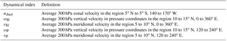
On the basis of long-term (1949–2011) correlations of the upper tropospheric zonal wind with the Southern Oscillation Index (SOI), Francey and Frederiksen (2016; hereafter FF16) defined an index for the Pacific westerly duct, uduct, as a measure of IH eddy transport of CO2. This index is the average zonal wind in the region 5∘ N to 5∘ S, 140 to 170∘ W at 300 hPa, as summarized in Table 1. In this article the period of interest is 1992 to 2016 and the corresponding correlation is shown in Fig. S1 of the Supplement. There the role of the changing Walker circulation with the cycle of the El Niño–Southern Oscillation (ENSO) in determining the properties of the Pacific and Atlantic westerly ducts is also documented. The uduct index is an indicator of cross-equatorial Rossby wave dispersion and associated increases in near-equatorial upper tropospheric transient kinetic energy (Frederiksen and Webster, 1988), particularly between 300 and 100 hPa (∼9 to ∼16 km above sea level). The process normally occurs over the eastern Pacific Ocean during the boreal winter–spring, and the Rossby waves (Webster and Holton, 1982; Stan et al., 2017), generated downwind of thermal anomalies and continental influences, in particular the massive Himalayan orography, propagate in a south-east direction through the Pacific westerly duct generating and transporting turbulent kinetic energy. The generation of turbulent kinetic energy occurs through Rossby wave breaking in the Pacific and Atlantic ducts and enhances turbulent mixing (Ortega et al., 2018 and references therein). FF16 also considered the relationship of uduct and other trace gases including CH4. Indeed, recently Pandey et al. (2017) and Krol et al. (2018) also considered the implications of faster IH transfer of CH4 during the La Niña of 2011 when the Pacific westerly wind duct was open and uduct was large.
FF16 explained the exceptional step in CO2 IH difference between 2009 and 2010 as being due to a contribution from the large anomaly in uduct observed at the time. Recently results from the National Aeronautics and Space Administration (NASA) Orbiting Carbon Observatory-2 (OCO-2) during the 2015–2016 El Niño have been published (Chatterjee et al., 2017; and references therein). In particular release by NASA (2016) of data in a video “Following Carbon Dioxide through the Atmosphere” provides further direct evidence of the Pacific duct hypothesis. The NASA OCO-2 CO2 concentration in Fig. 1a is for 17 February 2015 and shows Rossby wave trains over the eastern Pacific and across South America associated with IH exchange as a typical example of OCO-2 images that coincide with the shaded 2015 period in Fig. 1b. The dynamical properties of these Rossby waves are further explored in the Supplement, including Figs. S3 and S4. Figure 1b uses the covariance between CO2 and uduct in early 2015, indicated by shading, to predict IH CO2 exchange through the Pacific duct. The atmospheric circulation data and indices used throughout this article are obtained from the National Centers for Environmental Prediction (NCEP) and National Center for Atmospheric Research (NCAR) reanalysis (NNR) data (Kalnay et al., 1996); in Sect. 6 we briefly consider the robustness of our results using another reanalysis data set. The results in Fig. 1a and b are also consistent with upper tropospheric (u,v) wind vectors. Between 5 and 23 February 2015 NNR wind vectors show that a strong Pacific North American height anomaly caused a split in the Pacific upper tropospheric winds, the Pacific westerly duct was open, and there were south-east cross-equatorial winds from the Northern to Southern Hemisphere. This is illustrated in Fig. 1c for 300 hPa wind vectors on 17 February 2015.
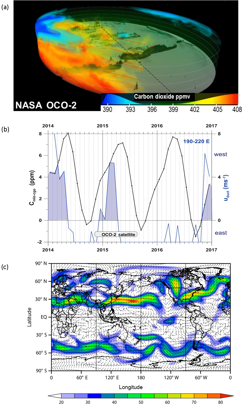
Figure 1(a) OCO-2 image for 17 February 2015 showing Rossby wave dispersion (dashed red lines) in CO2 concentration across the Equator (dotted black line). (b) Seasonal cycle of Cmlo−cgo and uduct, with area where both are positive shaded, for 1 January 2014 to 31 December 2016, and (c) 300 hPa wind vector directions and wind strength (ms−1) on 17 February 2015.
The focus here is on IH CO2 difference, anomalies in the mean convective and advective mode of IH CO2 exchange, and changes in the relative importance of the mean and eddy transport modes.
To represent the CO2 interhemispheric difference, we define Cmlo−cgo as the difference in Commonwealth Scientific and Industrial Research Organisation (CSIRO, 2018) analysed CO2 concentrations in baseline air sampled from Mauna Loa (mlo, 20∘ N, 156∘ W) and Cape Grim (cgo, 41∘ S, 145∘ E). FF16 discussed the measurement and sampling strategy, consistently applied over 25 years, which has been used to establish the data set with minimum uncertainty. They also examined the CO2 interhemispheric difference with the Scripps Institution of Oceanography (SIO) Mauna Loa and South Pole data (Keeling et al., 2009) and found broad agreement in the two data sets, in the period of overlap since the 1990s, in terms of CO2 changes and the relationships to the opening and closing of the Pacific westerly duct.
Figure 2 summarizes annual covariations that motivated this study. In Fig. 2a the overall trend in the Cmlo−cgo reflects the increasing emissions, mainly in the Northern Hemisphere, of carbon from combustion of fossil fuels coupled with relatively slow transport into the Southern Hemisphere. The smooth dashed curve shows global annual anthropogenic emissions (Le Quéré et al., 2018) scaled by the coefficients of linear regression between Cmlo−cgo and emissions from 1992 to 2015 (0.36 ppm (PgC)−1 yr, n=24, r2=0.83). The year-to-year variations in Cmlo−cgo are more pronounced than the variations in emissions (for example, only 2009, corresponding to the global financial crisis, clearly interrupts the smooth emissions increase).

Figure 2(a) Annual average Cmlo−cgo (solid) and global CO2 emission estimate (dashed) for 1992 to 2016, (b) Cmlo−cgo for boreal winter–spring (blue) and summer–autumn (orange), (c) uduct for boreal winter–spring (blue) and summer–autumn (orange), and (d) boreal summer–autumn ωH, (orange) and vH (green).
2.1 The influences of terrestrial fluxes and transport on interhemispheric CO2 differences
The growth rate and concentration of atmospheric CO2 depend on many mechanisms including fossil fuel emissions, surface fluxes, such as associated with the growth and decay of vegetation, and atmospheric mean and eddy transport. The CO2 growth rate and IH gradients in CO2 vary on daily, monthly, yearly, and multi-year timescales, where there is a quasi-periodic variability associated with the influence of ENSO (e.g. Thoning et al., 1989). This reflects the response of tropical vegetation to rainfall variations and both hemispheres are also affected through dynamical coupling.
A number of recent inversion studies have largely attributed growth anomalies in atmospheric CO2 concentrations to anomalous responses of the terrestrial biosphere. However, the variability in the responses within dynamic global vegetation models (DGVMs) is significant. Le Quéré et al. (2018), for example, note that the “standard deviation of the annual CO2 sink across the DGVMs averages to ±0.8 GtC year−1 for the period 1959 to 2016”. This is significantly larger than the reported extratropical sink anomalies during, for example, the major 2009–2010 step in CO2 concentrations (Poulter et al., 2014; Trudinger et al., 2016). Francey and Frederiksen (2015) presented reasons supporting a dynamical contribution to the cause of the 2009–2010 Cmlo−cgo step.
For the 2015–2016 period of particular relevance here there are two studies that stand out. Keenan et al. (2016) interpret slowing CO2 growth in 2016 as strong uptake by Northern Hemisphere terrestrial forests. Yue et al. (2017) examine the reasons for the strong positive anomalies in atmospheric CO2 growth rates during 2015. They present evidence of the Northern Hemisphere terrestrial response to El Niño events by way of satellite observations of vegetation greenness. To reconcile increased greenness with increased CO2 growth, their inversion modelling requires the “largest ever observed” transition from sink to source in the tropical biosphere at the peak of the El Niño, “but the detailed mechanisms underlying such an extreme transition remain to be elucidated”.
In this study, we find that the 2015–2016 El Niño also corresponds to unprecedented anomalies in both mean and eddy IH CO2 transport characterized by indices of these transfers that we introduce. As for the anomalies in CO2 IH gradient during the 2009–2010 El Niño, studied in FF16, this again suggests a contributing role for anomalous IH transport during the 2015–2016 event. We examine this possibility in detail and study the relationships between the extremes in IH CO2 differences and transport anomalies for 1992 to 2016 and associated correlations between Cmlo−cgo (and other trace gases) and dynamical indices of transport.
2.2 Dynamical influences on IH exchange
Figure 2b confirms that much of the year-to-year variability in Cmlo−cgo, particularly preceding 2010, occurs in the boreal winter–spring (December–May), when eddy transport is expected to make a more active contribution to IH exchange (FF16). The step jump in annual values between 2009 and 2010, which was the focus of FF16, is the most prominent feature. A similar relationship with uduct is supported prior to 2010 as indicated here by vertical dashed grid lines aligned with the beginning of the calendar years when uduct is unusually low (uduct≤3 ms−1). At these times uduct generally corresponds to above-average Cmlo−cgo, consistent with an accumulation of CO2 in the Northern Hemisphere at a time when the Pacific duct transfer is small.
A notable exception occurs in 2015–2016, and this is a particular focus of this study that we address in the context of the unusual Cmlo−cgo behaviour since 2010. For example, since 2010 the annual average Cmlo−cgo in Fig. 2a shows reduced scatter and a slight decrease at a time when fossil fuel emissions continue to grow. As shown in Fig. 2b, this Cmlo−cgo decrease is more marked in the boreal summer–autumn (June–November) than in boreal winter–spring (December–May) when it is relatively stable (and even recovers in the last 3 years).
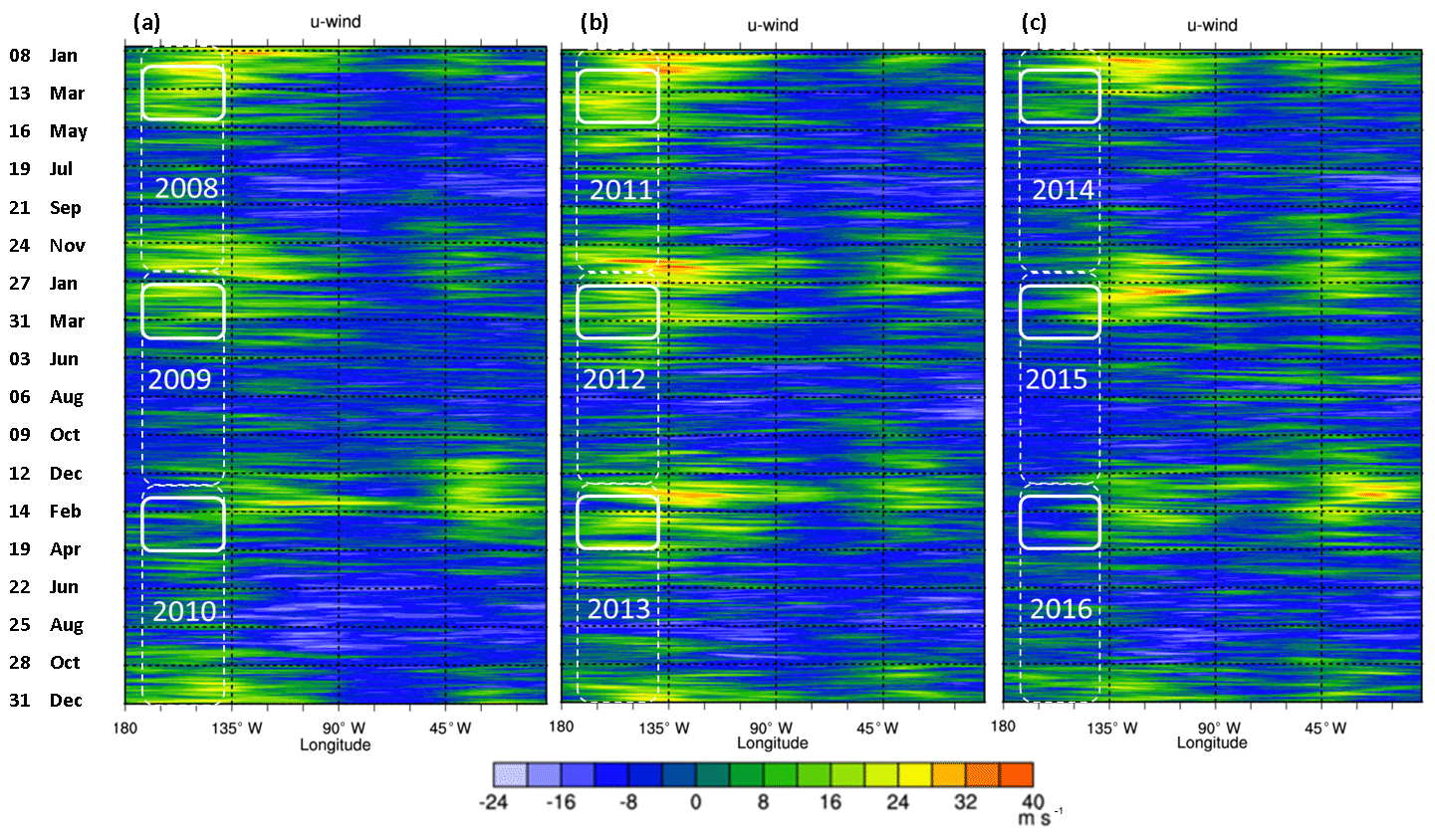
Figure 3Hovmöller diagrams of 300 hPa zonal wind (ms−1) averaged between 5∘ S and 5∘ N as a function of longitude and time for (a) 1 January 2008 to 31 December 2010, (b) 1 January 2011 to 31 December 2013, and (c) 1 January 2014 to 31 December 2016. Green through to red represent westerly winds (u winds, ms−1) over the Western Hemisphere. White solid rounded rectangles denote the longitudinal extent of the Pacific duct, and the height denotes the February to April period.
The steadily decreasing uduct since 2012 occurs all year round in Fig. 2c. Similar decreases occur in indices ωH and vH in Fig. 2d, which measure the strength and location of the Hadley circulation. Here, ωH is the 300 hPa vertical velocity in pressure coordinates ( where p is pressure) averaged zonally (0–360∘) and between 10 and 15∘ N (Table 1). Also, vH is the 200 hPa south–north meridional wind averaged zonally and between 5 and 10∘ N (Table 1). Both ωH and vH become more negative and the mean transport from the Northern to Southern Hemisphere increases with a strengthening of the Hadley circulation. As noted by Freitas et al. (2017; and references therein), the Hadley circulation strengthens during El Niños, and particularly for strong events such as during 2015–2016 (L'Heureux et al., 2017). There are subtle relationships between the latitudinal width of the equatorial heating during El Niño and global warming (Freitas et al., 2017) and the Hadley circulation. However, it is expected that there will be an increasing frequency of extreme El Niño events with increasing global warming (Cai et al., 2014; Yeh et al., 2018).
Before examining the Hadley component further, we clarify factors associated with the eddy transfer through the Pacific duct.
We examine here the concept of relatively rapid interhemispheric CO2 exchange through a spatially restricted Pacific duct and discuss issues of the uniqueness of the duct and the transport of both turbulent kinetic energy and CO2 to and through the Pacific duct region.
3.1 Eddy generation in the equatorial zone
The uduct zonal wind based on the peak climatological correlation with SOI (140–170∘ W) is also largely representative of near-equatorial (5∘ N to 5∘ S) zonal winds and their variability in the larger region between 90∘ W and 180∘. Pattern correlations between the two vary from r∼0.9 for November to April to r∼0.7 for May to October.
In Fig. 3, Hovmöller diagrams for the Western Hemisphere (180 to 0∘ W) between 2008 and 2016 show the time–longitude of daily 300 hPa zonal winds between 5∘ N and 5∘ S. The cool blue background represents easterly winds (negative u), while warm colours, green to yellow through to red, depict westerlies (positive u). Frederiksen and Webster (1988) found that near-equatorial upper tropospheric transient kinetic energy generation is approximately linearly related to zonal wind strength (their Fig. 6) and is strongest for westerlies when the winds oppose the earth's rotation. The longitudinal limits of uduct determined from the SOI correlation are enclosed by solid white rounded rectangles in Fig. 3, while the time period (rectangle height) represents those months when Cmlo−cgo is at a seasonal maximum and winds in the Pacific duct are normally westerly (February–April).
In most years, uduct is positive in boreal winter–spring and Rossby waves generated by, for example, the Himalayas (height of 8.8 km) can propagate through the downstream Pacific duct region (140–170∘ W, 5∘ N–5∘ S), producing and transporting turbulent kinetic energy southwards. In some years, such as the boreal winter–spring of 2009–2010 and 2015–2016, uduct is anomalously weak and the peak equatorial 300 hPa zonal winds are over the Atlantic Ocean, particularly in the Atlantic duct region defined as 10–40∘ W, 5∘ N–5∘ S. The Atlantic duct region, most conspicuously, is downstream of the Rockies (height of 4.4 km). Our Fig. S1 and Fig. 4a of FF16 show that the SOI and Atlantic duct zonal winds are strongly anti-correlated in contrast to the strong correlation with uduct; in the Eastern Hemisphere the correlation between the SOI and equatorial zonal winds is quite weak as well. We note that uduct and the Atlantic duct winds are anti-correlated with . Further, while uduct is anti-correlated with Cmlo−cgo, the Atlantic duct winds are correlated with a similar magnitude. This indicates that changes in uduct are the primary determinant of interhemispheric CO2 duct transfer via eddy processes and Cmlo−cgo and the opening of the Atlantic duct is mainly important through the associated closing of the Pacific duct. This is consistent with the idea that Rossby wave dispersion from the smaller topographic features of the Rockies is less important than from the comparatively massive Himalayas, as further discussed in the Supplement.

Figure 4Correlation of vertical velocity ω (Pas−1) at 300 hPa with SOI for February–April and 1948–2016.
3.2 Transport of surface CO2 emissions to the upper troposphere
Transport of CO2 emissions from the surface to the upper troposphere is explored next. We find that when the Pacific duct is open there is also large-scale uplift slightly downstream of Asia so that in a given winter–spring season the substantial regional emissions are effectively transported directly through the duct via Rossby wave dispersion, including by the Himalayan wave train. Figure 4 shows the February–April correlation between the 500 hPa ω (the vertical wind in pressure coordinates with negative values corresponding to uplift in height coordinates) and the SOI from 1948 to 2016. The most prominent correlations occur within ±30∘ of the Equator at longitudes 120∘ E to 170∘ W, upstream, and at the longitudes of the Pacific duct, and this is in fact the case at all levels between the surface and 100 hPa (not shown). Broadly similar correlations are obtained between the 500 hPa ω and uduct for February–April (and for 500 hPa ω and SOI for January–December). At other times, for example in 2010 and 2015–2016, when there have been persisting easterlies in the Pacific duct region, there has been descent slightly downstream of the Asian region. Thus the recent record Asian emissions may play a significant role in direct episodic IH CO2 transfer through the Pacific duct. To the extent that Asian emissions might be preferentially represented in direct IH CO2 transfer, it is relevant that uncertainty and possibly variability in Asian emissions are greater than the reported uncertainty and variability in the global totals (Andres et al., 2014).

Figure 5Latitude–height cross section of June to August 120–240∘ E average (a) ω (Pas−1) – vertical velocity in pressure coordinates – for 1979–2016, (b) ω difference of 2016 minus 1979–2016, and(c) ω difference of 2016 minus 2010.
As noted in Sect. 2, the years 2010 and 2016 exhibit a similar anomalous eddy transport index, uduct, but have different Cmlo−cgo responses relative to previous years (Fig. 2a). Since the CO2 emitted in the Northern Hemisphere and tropics is also transported into the Southern Hemisphere by the mean divergent flow associated with the Hadley circulation, particularly during boreal summer (Miyazaki et al., 2008), this is now explored in more detail. The Pacific duct transfer in boreal winter–spring, with peaks in February–April, occurs when the CO2 IH partial pressure difference is near the maximum due to forest respiration. Likewise the mean IH transport related to the Hadley circulation occurs in boreal summer–autumn, with peaks in June–August, when the CO2 IH partial pressure difference has a proportionally larger contribution due to the accumulated fossil fuel CO2 from NH industrial emissions.
Figure 5 shows latitude–height cross sections, over the Pacific, averaged between 120 and 240∘ E, of June to August vertical wind in pressure coordinates, ω, while Fig. 6 shows the corresponding results for the meridional wind, v. Recall that negative ω corresponds to positive vertical velocity in height coordinates and negative v is north–south meridional wind. In the boreal summer–spring, average values for 1979 to 2016 show the uplift (negative ω) at low northern latitudes (Fig. 5a), while the advective Hadley cell meridional transfer (negative v) to the Southern Hemisphere at high altitude can be seen in Fig. 6a.
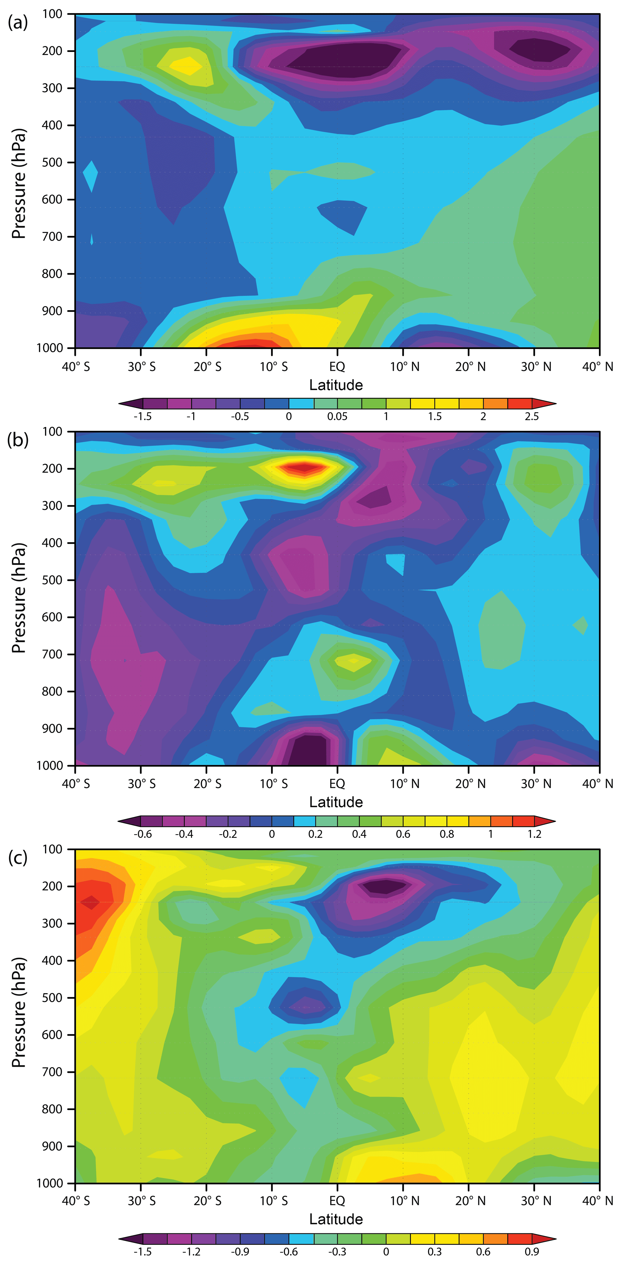
Figure 6Latitude–height cross section of June to August 120–240∘ E average (a) meridional wind v (ms−1) for 1979–2016, (b) meridional wind v difference of 2016 minus 1979–2016, and (c) meridional wind v difference of 2016 minus 2010.
By subtracting the 1979–2016 average from the 2016 ω values and v values, the nature of the extreme 2016 anomaly becomes visible, with strong uplift including between 10 and 15∘ N shown in Fig. 5b and extensive meridional wind penetration into the Southern Hemisphere, particularly between 500 and 300 hPa, shown in Fig. 6b.
Figures 5c and 6c depict the difference between the anomaly years 2016 and 2010. Both the uplift between 10 and 15∘ N and penetration of the meridional wind into the Southern Hemisphere is stronger in the upper troposphere and mean transport through convection and advection into the Southern Hemisphere more extensive in 2016.
On the basis of these figures, and similar figures for the corresponding zonally averaged quantities, we have chosen four indices to characterize the mean circulation by the Hadley cell (Table 1). These are ωP, the vertical velocity in pressure coordinates over the Pacific Ocean at 300 hPa averaged between 120–240∘ E and 10–15∘ N, and vP, the meridional wind at 200 hPa averaged between 120–240∘ E and 5–10∘ N, as well as the corresponding zonally averaged indices ωH and vH introduced in Sect. 2.
The timing of a majority of short term variations in the 25-year baseline Cmlo−cgo corresponds to atmospheric transport changes that influence the interhemispheric exchange. To quantify relationships between Cmlo−cgo and the eddy and mean transport indices involved, we first suppress the Cmlo−cgo changes expected from reported anthropogenic emissions. The global annual average anthropogenic emissions (Le Quéré et al., 2018) are converted to ppm using the coefficient 0.36 ppm (PgC)−1 yr derived in Sect. 2 from Fig. 2 and subtracted from the observed Cmlo−cgo. In Fig. 6 we compare the FF-adjusted Cmlo−cgo, which we denote , for two periods when Cmlo−cgo is positive; the first is February–April that best captures the eddy IH exchange, and the second is June–August when mean transfer related to the Hadley circulation is captured.
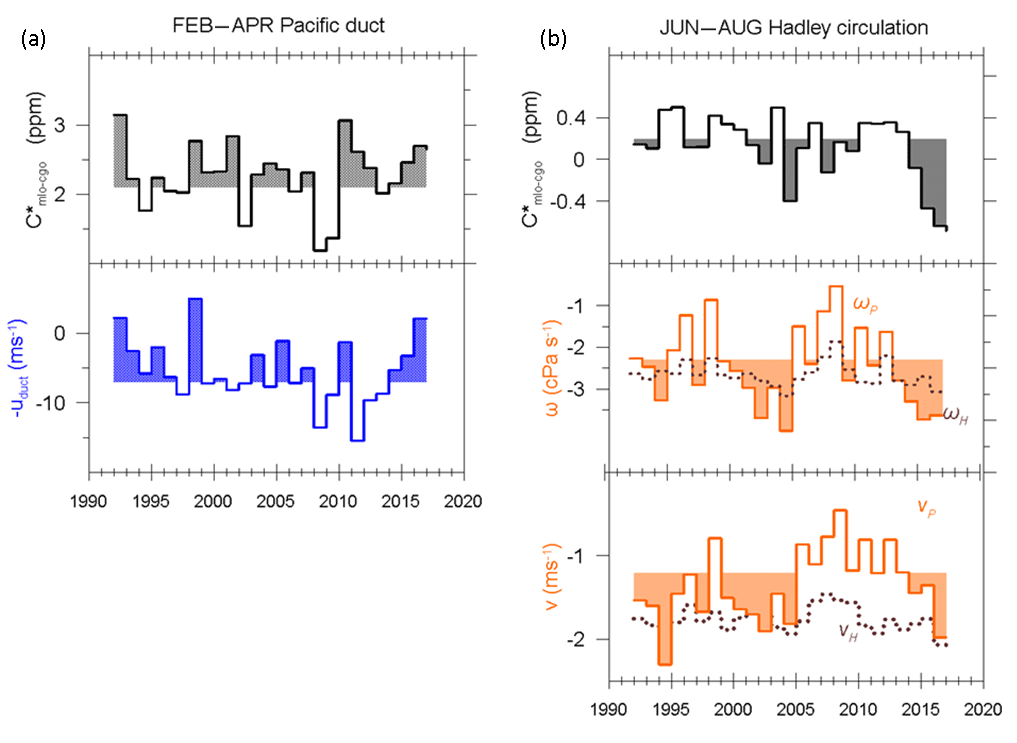
Figure 7(a) and −uduct averaged between February and April for 1992–2016 and (b) , ωP, ωH, vP, and vH averaged between June and August for 1992–2016.
We focus first on the FF-adjusted plots in Fig. 7a and b. The mean and year-to-year variation is very much larger in (a) compared to (b) and is also larger in (a) compared to the annual averaged values in Fig. 2a. The contrasting behaviour between the two periods after 2012 is also more marked.
To emphasize the similarities between and Pacific duct winds, we plot −uduct in Fig. 7a, so that easterlies are shown as positive and the more frequent westerlies as negative; the timings of peaks in both panels then correspond to each other. When winds in the Pacific duct are easterly or near zero, FF-adjusted peak or are above average; this is now more obvious in 2016 compared with the corresponding results for Cmlo−cgo in December–May shown in Fig. 2b and c. In fact the FF-adjusted has very similar behaviour to the detrended Cmlo−cgo, with pattern correlations of anomalies of r=0.931, r=0.954, and r=0.981, for January–December, June–August, and February–April respectively. The similarity can also be seen by comparing the top panel of Fig. 7b with that of Fig. 8. Despite persistent agreement in timing, the magnitude of the Cmlo−cgo response to the uduct anomaly is more variable. This is reflected in the correlation between the detrended Cmlo−cgo anomalies and the detrended uduct anomalies, which is for February–April and for December–May. These results confirm the preferential Pacific duct transfer in late boreal winter and early spring (February–April). They also indicate that although there is an important relationship between Cmlo−cgo and the zonal wind in the Pacific duct, other processes detailed in Sect. 2, such as changes in direct advective transport by the mean winds and emissions, also play roles in year-to-year IH variations. This is also confirmed by a regression analysis of Cmlo−cgo anomalies onto uduct anomalies (not shown), where there is significant scatter about the regression line.
In particular, during 2009–2010 there were a number of complicating factors that most likely contributed to this. The unusually low Cmlo−cgo in 2008 and 2009 coincide with the global financial crisis when global emissions dipped (and recent estimates of emissions by British Petroleum, 2018, suggest an even larger 2008–2009 anomaly than in data used here). Terrestrial net biosphere production south of 30∘ S was also anomalously low in 2009 and anomalously high in 2010 (FF16; Trudinger et al., 2016; though by amounts not sufficient to impact on the Cape Grim baseline CO2 records). The low Cmlo−cgo also align with near-record strong westerlies in the Pacific duct, and associated larger eddy transport, in 2008; both potentially contribute to an increase in the magnitude of the subsequent CO2 step.
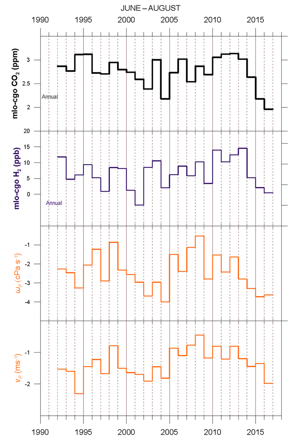
Figure 8Time series of June–August and annual averages of detrended mlo–cgo differences in CO2 and H2 and June–August average dynamical indices ωP and vP.
In Fig. 7b the post-2010 decrease in June–August FF-adjusted is clearly mirrored in the decreasing ω and v indices (indicating strengthened Hadley circulation), particularly in the 120–240∘ E Pacific sector (ωP and vP) compared to the zonal average (ωH and vH). The considerably weaker strength of the Hadley circulation in 2010 compared with 2016 is shown quite distinctly. The correlations between the detrended Cmlo−cgo anomalies and indices of mean transport are shown in Table 2.
Table 2Correlations (r) between the detrended Cmlo−cgo anomalies and indices of mean transport ωH, ωP, vH, and vP, averaged for June–August and June–November 1992–2016.
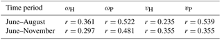
Generally June–August correlations are stronger than the June–November correlations, and correlations over the Pacific sector 120–240∘ E are generally larger than for the zonally averaged quantities. This is clearly the case for ω, while vH is an exception, being larger for the longer time period. The Cmlo−cgo correlations for June–August involving ωP and vP have roughly similar magnitudes to those for February–April, involving uduct, and ωP and vP provide similar predictability of the role of the Hadley circulation in mean IH CO2 transport as uduct does for eddy transport. Interestingly, during 2009–2010 the effects of uduct and ωP and vP reinforce one another to make the step in Cmlo−cgo large, while for 2015–2016 ωP and vP counteract uduct, and the exceptionally strong Hadley circulation becomes the dominant feature in determining the annual Cmlo−cgo (Fig. 1a). These results show that there is an important connection between the Cmlo−cgo and the indices that characterizes the strength of the Hadley circulation and mean transport. Again, as also suggested by regression analysis (not shown), other processes, detailed in Sect. 2 and above, also play important roles.
The somewhat different behaviours of Cmlo−cgo and the dynamical indices, particularly during the El Niños of 2009–2010 and 2015–2016 and of 1997–1998, may partly reflect the diversity of El Niños and whether the heating is focussed in the eastern Pacific or in the central Pacific (Capotondi et al., 2015; L'Heureux et al., 2017 and references therein). The strong 1997–1998 event, like the 1982–1983 event, was a classic eastern Pacific El Niño, with maximum temperature anomalies of nearly +4 ∘C (L'Heureux et al., 2017). The 2009–2010 event, in contrast, was a central Pacific El Niño, with record-breaking warming in the central Pacific (Kim et al., 2011). The 2015–2016 El Niño fell between these two canonical cases, with less warming in the eastern Pacific Ocean than the 1997–1998 event, but similar warming to the 2009–2010 event in the central Pacific (L'Heureux et al., 2017).
The broadly increasing magnitude of the negative ω and v indices since 2012 is associated with both increasing global temperatures, breaking the record in 2016, and the large El Niño of 2015 and 2016. This has resulted in the increasing importance of the mean convective and advective CO2 transport by the Hadley circulation relative to the eddy transport including through the Pacific duct. It will be interesting to see whether this favouring of the mean over the eddy IH CO2 transport will become increasingly important with further global warming and the extent to which it depends on extreme El Niños (Cai et al., 2014; Freitas et al., 2017; Yeh et al., 2018).
The dynamical indices that we have used for this study are based on the NCEP-NCAR reanalysis (NNR) data (Kalnay et al., 1996). There is generally close correspondence between the major global atmospheric circulation data sets that, like the NNR data, use full data assimilation throughout the atmosphere (Frederiksen and Frederiksen, 2007; Frederiksen et al., 2017a; Rikus, 2018). We have confirmed this by recalculating our dynamical indices and main correlations with Cmlo−cgo based on the NASA Modern Era Retrospective-analysis for Research and Applications (MERRA) data (Rienecker et al., 2011). For example, the 1992 to 2016 correlation between MERRA and NNR data for uduct in February–April is r=0.974, for ωP in June–August is r=0.899, and for vP in June–August is r=0.931. The corresponding correlations between detrended anomalies of Cmlo−cgo and the MERRA-based dynamical indices are also very similar. The correlations are with uduct for February–April (compared with for the NNR index), r=0.504 with ωP for June–August (compared with r=0.522 based on NNR), and r=0.538 with vP for June–August (compared with r=0.539 based on NNR).
Next, we consider the eddy and mean IH exchange of other trace gas species and their correlations with CO2 and dynamical indices of transport. We focus on February–April for eddy transport and June–August for mean transport since these periods were the peaks for correlations of CO2 IH difference with eddy and mean transport indices respectively. However, there are differences in the seasonal variability of the interhemispheric gradient in the different trace gas species that are reflected in their transport, and for that reason we also briefly mention the results for other time periods. We begin by further examining Mauna Loa minus Cape Grim (mlo–cgo) differences, between 1992–2016, in the routinely monitored CSIRO species (CSIRO, 2018) CH4, CO, and H2 in addition to CO2 that were briefly considered by Francey and Frederiksen (FF16), as well as N2O (for 1993–2016). Thereafter we discuss mlo–cgo differences in SF6 data sourced from the NOAA Halocarbons and other Atmospheric Trace Species Group (HATS) program from 1998 (NOAA, 2018).
6.1 Pacific westerly duct and eddy IH transport of CSIRO-monitored trace gases
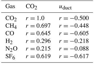
The IH exchange of the trace gas species, CH4, CO, and H2, in addition to CO2, and the role of the Pacific westerly wind duct were also considered in FF16. In particular, the covariance, of the mlo–cgo difference in these routinely monitored CSIRO species with uduct, is shown in Fig. 5 of FF16. We recall that the uduct index is the average zonal wind in the region 5∘ N to 5∘ S, 140 to 170∘ W at 300 hPa. As noted in FF16, the extreme cases of Pacific westerly duct closure in 1997–1998 and 2009–2010 show up in the reduction of seasonal IH exchange for CH4 and CO as well as CO2. The similar behaviour of detrended anomalies of mlo–cgo difference in CH4, CO, and CO2 and their correlations with uduct is shown in Table 3 for February–April. We note the quite high correlations of CH4 and CO with CO2 (r=0.697 and r=0.645 respectively) and the significant anti-correlations of all these three species with , and respectively). In fact, for March–May the correlation between CH4 and CO2 is even larger at r=0.728 (and with uduct it is ), while between CO and CO2 it is r=0.611 (and with uduct it is ). These results are of course consistent with Fig. 5 of FF16 and are further evidence of similarities of IH transient eddy transport of these three gases. Table 3 also shows that the February–April correlation of H2 with CO2 and anti-correlation with uduct have smaller magnitudes (r=0.296 and , respectively). These results for anomalies are probably related to corresponding similarities and differences in the seasonal mean values (not shown) of these gases in February–April, as discussed below.
Table 3Correlations (r) between the detrended mlo–cgo gas anomalies for CO2, CH4, CO, and H2 with CO2 and uduct index of transient transport averaged between February and April for 1992–2016. Also shown are corresponding correlations for N2O and 1993–2016 and for SF6 and 1998–2012.
Anomalies in mlo–cgo differences in CSIRO-monitored N2O are generally poorly correlated with those in CO2 as shown for February–April and June–August in Tables 3 and 4 respectively (the maximum 3-month average correlation is r=0.274 for March–May), and this is mirrored in generally poor correlation with the dynamical indices shown in Tables 3 and 4. This reflects the fact that natural exchanges with equatorial agriculture and oceans are the main sources (Ishijima et al., 2009), and the seasonal range in mlo–cgo difference is only around 0.2 % of the mean N2O level, more than 10 times less than is the case for the other species.
6.2 Hadley circulation and mean IH transport of CSIRO-monitored trace gases
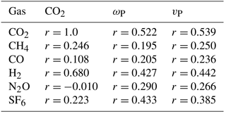
We examine the role of the Hadley circulation in the mean transport of trace gases focusing on the boreal summer period of June–August. Table 4 shows the correlations between the detrended anomalies of mlo–cgo difference in CH4, CO, and H2 with CO2 and with the dynamical indices ωP and vP (Table 1). We note that the largest June–August correlation is between H2 and CO2 (r=0.680) and the correlations between CH4 and CO with CO2 are considerably smaller (r=0.246 and r=0.108, respectively), while for April–June the latter correlations are more comparable at r=0.583 and r=0.496 respectively.
These correlations with CO2 are also reflected in the respective correlations of the other trace gases with ωP and vP. We note from Table 4 that the June–August correlations of H2 with ωP and vP are r=0.427 and r=0.442 respectively, which is slightly less than the corresponding correlations between CO2 and the dynamical indices (r=0.522 and r=0.539, respectively), but considerably larger than for CH4 and CO. For May–July the correlation of H2 with ωP is slightly larger, with r=0.526.
Again, the different behaviour of the trace gas anomalies may be related to their different seasonal mean values; the seasonal mean IH difference for H2 peaks in boreal summer, while for CH4 and CO, it is relatively low with a minimum in August. The distribution and variability of surface exchange is different for each of the trace gases and there is potential for this to interact with the restricted extent and seasonal meandering of the regions of uplift to influence IH exchange of a species. For example, 70 % of the global total CH4 emissions are from mainly equatorial biogenic sources that include wetlands, rice agriculture, livestock, landfills, forests, oceans, and termites (Denman et al., 2007), and CO emissions receive a significant contribution from CH4 oxidation and from tropical biomass burning.
Table 4Correlations (r) between the detrended mlo–cgo gas anomalies for CO2, CH4, CO, and H2 with CO2 and indices of mean transport, ωP, and vP averaged between June–August for 1992–2016. Also shown are corresponding correlations for N2O and 1993–2016 and for SF6 and 1998–2012.
A more detailed examination of the inter-annual variation of the mlo–cgo difference in H2 during boreal summer is presented in Fig. 8. It shows the detrended H2 data in comparison with the corresponding CO2 data and with the ωP and vP indices.
First we note that the detrended CO2 data in the top panel have very similar inter-annual variation to the FF-adjusted in Fig. 7b. We also see that the qualitative behaviour of H2 mirrors many aspects of CO2, as expected from the correlations in Table 4. In particular, the increase in the IH difference of H2 in 2010 is even more pronounced than for CO2. For CO2 and for H2 there is a steady reduction in the IH difference from around 2013, leading to a local minimum in 2016. In both of these respects these gases broadly follow the changes in the Hadley circulation, including the strengthening during 2015–2016. Vertical lines in Fig. 8 indicate other times between 1992 and 2016 when transitions occur in both these trace gases and in the Hadley circulation characterized by ωP and vP.
Surface exchanges of H2 have similarities to those of CO2 in that they occur mostly at mid–northern latitudes and are mainly due to emissions from fossil fuel combustion. However H2 also has mid–northern-latitude photochemical sources peaking in August (Price et al., 2007). These boreal summer sources are almost offset by a combined soil and hydroxyl sink, but the overall interhemispheric partial pressure difference is boosted by a significant reduction in the Southern Hemisphere photochemical source at that time. For both species, the most northern excursions of the intertropical convergence zone that occurs at Pacific latitudes encounter increasing concentrations of both gases.
As noted above, anomalies in mlo–cgo differences in N2O are poorly correlated with those in CO2 and in dynamical indices (Tables 3 and 4). Indeed the 3-month average anti-correlation with uduct that has the largest magnitude is for March–May and the largest correlation with ωP is r=0.359 for April–June and with vP is r=0.350 for May–July.
6.3 Interhemispheric exchange of SF6
In the case of SF6 we have analysed the mlo–cgo difference in available NOAA HATS data from 1998 to 2012 when cgo HATS measurements ceased. Correlations (Tables 3 and 4) of detrended anomalies in IH differences in SF6 with those in CO2 are as follows: the February–April correlation is r=0.619, the March–May correlation is r=0.722, the April–June correlation is r=0.595, the May–July correlation is r=0.303, and the June–August correlation is r=0.223. The corresponding correlations with dynamical indices are as follows: for February–April the correlation with uduct is , the May–July correlations with ωP is r=0.465, the June–August correlation with ωP is r=0.433, the May–July correlation with vP is r=0.517, and the June–August correlation with vP is r=0.385. We note that SF6 has an anti-correlation with uduct for February–April that has a larger magnitude than for CO2 and even CO. Thus, again there is a significant influence of the Pacific westerly duct, in late boreal winter and spring, and of the Hadley circulation, in boreal summer and late spring, as measured by these indices, on the mlo–cgo differences of SF6; these SF6 differences exhibit a similar step change in 2009–2010 as shown for CO2 in Figs. 2 and 7.
The major El Niño of 2015 and 2016 coincided with record global warming, with 2016 having the highest global average surface temperatures and 2015 the third highest (2017 had the second highest). The strength of the Hadley circulation also increased to unprecedented levels during 2015–2016 and had a major impact on the mean interhemispheric (IH) transport of CO2 and on the difference in CO2 concentration between Mauna Loa and Cape Grim (Cmlo−cgo). This study has focussed on the roles of IH transient eddy and mean transport of CO2 on interannual variations in Cmlo−cgo and has established dynamical indices that characterize the broad features of this transfer (Table 1). Interestingly, some of these indices are based on regions that lie close to or overlap the region of the Niño 3.4 sea surface temperature (SST) index (the average SST in the region 5∘ N–5∘ S, 120–170∘ W), where ENSO is strongly coupled to the overlying atmosphere (L'Heureux et al., 2017).
One of these indices, uduct, which is a measure of eddy IH transport of CO2, was introduced in FF16. This index is the 300 hPa Pacific zonal wind averaged between 5∘ N–5∘ S and 140–170∘ W and is strongly correlated with the Southern Oscillation (SOI) index (r∼0.8 in Fig. 4a of FF16). A particular focus of that study was to propose an explanation for the record step in CO2 IH difference between 2009 and 2010 and it was concluded that the closing of the Pacific duct (negative uduct) during the El Niño of 2010 was a significant contributing factor. It was also noted that there were half a dozen other occasions going back to the 1960s when the closing of the Pacific duct was related to an increase in CO2 IH difference (Keeling et al., 2009).
Here, we have extended the analysis of the relationship between uduct and Cmlo−cgo to 2016. We again find that during boreal winter–spring, and particularly during February–April when eddy transport of CO2 from the Northern to Southern Hemisphere is most active, there is an increase in Cmlo−cgo during the El Niño of 2015–2016. However, while the timing of the increases in these years, and for other occasions going back to 1992, agree with the closing of the Pacific duct, the magnitude is more variable, indicating the contribution of other processes discussed in Sect. 2. We have analysed the intermittent nature of the opening and closing of the Pacific westerly duct. In particular, episodes in February 2015 have been related to results from NASA (2016) data in the video “Following Carbon Dioxide through the Atmosphere”. The video provides further evidence of the propagation of Rossby waves through the open Pacific westerly duct and the transfer of CO2 into the Southern Hemisphere. We have also noted that large-scale uplift slightly downstream of Asia occurs when the Pacific duct is open, allowing these substantial emissions to be transported directly, via Rossby wave dispersion, through the duct.
A major focus of this article has also been the role of changes in the mean IH CO2 transport from the Northern to Southern Hemisphere due to variability in the Hadley circulation. We have introduced indices (Table 1) that measure this transfer based on the 300 hPa ω, the vertical velocity in pressure coordinates, between 10 and 15∘ N and 200 hPa v, the meridional wind between 5 and 10∘ N, both zonally averaged (ωH and vH) and with averaging restricted to the Pacific sector 120–240∘ E (ωP and vP). The correlations for June–August between Cmlo−cgo and ωP or vP(r∼0.5) have roughly similar magnitudes to those in February–April involving uduct. The indices ωP and vP provide similar predictability of the role of the Hadley circulation in mean IH CO2 transport as uduct does for eddy transport. We have also found that during 2009–2010, the effects of uduct and ωP and vP reinforce one another to make the step in Cmlo−cgo large. In contrast, for 2015–2016 ωP and vP counteract uduct, and the record Hadley circulation primarily determines the annual Mauna Loa and Cape Grim CO2 difference. The effects of interannual changes in mean and eddy transport on IH gradients in CO2 (and CH4, CO, H2, N2O, and SF6) have been examined for the period 1992 to 2016.
The sign and strength of zonal winds in the Pacific westerly duct (uduct) are related to Rossby wave dispersion and breaking and are correlated with corresponding changes in near-equatorial transient kinetic energy (Fig. 6; Frederiksen and Webster, 1988), resulting in intermittent changes in the mixing of trace gases. This effect may not be adequately represented in the parameterizations (Frederiksen et al., 2017b) used in atmospheric circulation and transport models. Model determinations of short-term variations in the Hadley circulation exchange are also susceptible to uncertainties in representations of the equatorial convective dynamics (Lintner et al., 2004). Over at least 25 years, much of the variability in CO2 between the two surface monitoring sites of Mauna Loa and Cape Grim can be associated with dynamical near-equatorial atmospheric indices of global significance in a changing climate. The changing nature of the seasonal and inter-annual changes in CO2 IH Pacific duct eddy and mean Hadley circulation transfer between 1992 and 2016 provides an interesting case study and potential test of inversion models of atmospheric transport.
We plan to further explore trace gas IH transfer focussing on Southern Hemisphere CO2 stable isotope data in a study that distinguishes between mean IH transfer and eddy transfers of both current season emissions and accumulated Northern Hemisphere fossil fuel emissions.
Meteorological data are available from the NOAA/ESRL website at http://www.esrl.noaa.gov/psd/ (Kalnay et al., 1996) and from the NASA website at https://giovanni.gsfc.nasa.gov/giovanni/ (Rienecker et al., 2011), trace gas data for CSIRO-monitored species CO2, CH4, CO, H2 and N2O are available from the CSIRO website at ftp://gaspublic:gaspublic@pftp.csiro.au/pub/data/gaslab/ (CSIRO, 2018) and the NOAA-monitored SF6 data are available from the NOAA website at ftp://ftp.cmdl.noaa.gov/hats/sf6/flasks/Otto/monthly/ (NOAA, 2018).
The supplement related to this article is available online at: https://doi.org/10.5194/acp-18-14837-2018-supplement.
JSF provided information on atmospheric dynamics and the roles of transport mechanisms, and RJF provided the trace gas information. Both contributed to the writing of the paper.
The authors declare that they have no conflicts of interest.
We thank Nada Derek and Stacey Osbrough for assistance with the graphics and
Paul Steele for providing valuable advice on the manuscript. The sustained
focus and innovation of CSIRO GASLAB personnel, and skilled trace gas sample
collection by personnel at the Bureau of Meteorology Cape Grim Baseline
Atmospheric Program and NOAA's Mauna Loa stations underpin the progress
reported here. The dynamics contributions were prepared using data and
software from the NOAA/ESRL Physical Sciences Division website at
http://www.esrl.noaa.gov/psd/ except, as stated in Sect. 6, where NASA
MERRA data were also used from the website at
https://giovanni.gsfc.nasa.gov/giovanni/ . We acknowledge NASA Goddard
Flight Center and their Production Team for the video “Following Carbon
Dioxide through the Atmosphere” available on the website at
https://svs.gsfc.nasa.gov/12445 (last access:
11 October 2018).
Edited by: Martin Heimann
Reviewed by: Prabir K. Patra,
Abhishek Chatterjee,
and one anonymous referee
Andres, R. J., Boden, T. A., and Higdon D.: A new evaluation of the uncertainty associated with CDIAC estimates of fossil fuel carbon dioxide emission, Tellus B, 66, 23616, https://doi.org/10.3402/tellusb.v66.23616, 2014.
Bowman, K. P. and Cohen, P. J.: Interhemispheric exchange by seasonal modulation of the Hadley circulation, J. Atmos. Sci., 54, 2045–2059, 1997.
British Petroleum: CO2 emissions, available at: https://www.bp.com/en/global/corporate/energy-economics/statistical-review-of-world-energy/co2-emissions.html (last access: 30 March 2018), 2018.
Cai, W., Borlace, S., Lengaigne, M., van Rensch, P., Collins, M., Vecchi, G., Timmermann, A., Santoso, A., McPhaden, M. J., Wu, L., England, M. H., Wang, G., Guilyardi, E., and Jin, F. F.: Increasing frequency of extreme El Niño events due to greenhouse warming, Nat. Clim. Change, 4, 111–116, https://doi.org/10.1038/nclimate2100, 2014.
Capotondi, A., Wittenberg, T., Newman, M., Lorenzo, E. D., Yu, J. Y., Braconnot, P., Cole, J., Dewitte, B., Giese, B., Guilyardi, E., Jin, F. F., Karnauskas, K., Kirtman, B., Lee, T., Schneider, N., Xue, Y., and Yeh, S. W.: Understanding ENSO diversity, B. Am. Meteorol. Soc., 96, 921–938, https://doi.org/10.1175/BAMS-D-13-00117.1, 2015.
Chatterjee, A., Gierach, M. M., Sutton, A. J., Feely, R. A., Crisp, D., Eldering, A., Gunson, M. R., O'Dell, C. W., Stephens, B. B., and Schimel, D. S.: Influence of El Niño on atmospheric CO2 over the tropical Pacific Ocean: Findings from NASA's OCO-2 mission, Science, 358, eaam5776, https://doi.org/10.1126/science.aam5776, 2017.
CSIRO: CSIRO Oceans and Atmosphere GASLAB data October 2018, Commonwealth Scientific and Industrial Research Organisation, available at: ftp://gaspublic:gaspublic@pftp.csiro.au/pub/data/gaslab/ (last access: 10 October 2018), 2018.
Denman, K. L., Brasseur, G., Chidthaisong, A., Ciais, P., Cox, P. M., Dickinson, R. E., Hauglustaine, D., Heinze, C., Holland, E., Jacob, D., Lohmann, U., Ramachandran, S., da Silva Dias, P. L., Wofsy, S. C., and Zhang, X.: Couplings Between Changes in the Climate System and Biogeochemistry, in: Climate Change 2007: The Physical Science Basis. Contribution of Working Group I to the Fourth Assessment Report of the Intergovernmental Panel on Climate Change, edited by: Solomon, S., Qin, D., Manning, M., Chen, Z., Marquis, M., Averyt, K. B., Tignor, M., and Miller, H. L., Cambridge University Press, Cambridge, United Kingdom and New York, NY, USA, 2007.
Francey, R. J. and Frederiksen, J. S.: Interactive comment on “The 2009–2010 step in atmospheric CO2 inter-hemispheric difference” by R. J. Francey and J. S. Frederiksen, available at: https://www.biogeosciences-discuss.net/12/C7771/2015/bgd-12-C7771-2015-supplement.pdf, Biogeosciences Discuss., 12, C7771–C7771, 18 November 2015.
Francey, R. J. and Frederiksen, J. S.: The 2009–2010 step in atmospheric CO2 interhemispheric difference, Biogeosciences, 13, 873–885, https://doi.org/10.5194/bg-13-873-2016, 2016.
Frederiksen, J. S. and Frederiksen, C. S.: Interdecadal changes in Southern Hemisphere winter storm track modes, Tellus A, 59, 599–617, 2007.
Frederiksen, J. S. and Webster, P. J.: Alternative theories of atmospheric teleconnections and low-frequency fluctuations, Rev. Geophys., 26, 459–494, 1988.
Frederiksen, C. S., Frederiksen, J. S., Sisson, J. M., and Osbrough, S. L.: Trends and projections of Southern Hemisphere baroclinicity: The role of external forcing and impact on Australian rainfall, Clim. Dynam., 48, 3261–3282, https://doi.org/10.1007/s00382-016-3263-8, 2017a.
Frederiksen, J. S., Kitsios, V., O'Kane, T. J., and Zidikheri, M. J.: Stochastic subgrid modelling for geophysical and three-dimensional turbulence, in: Nonlinear and Stochastic Climate Dynamics, Chapter 9, 241–275, edited by: Franzke, C. J. E. and O'Kane, T. J., Cambridge University Press, 2017b.
Freitas, A. C. V., Frederiksen, J. S., O'Kane, T. J., and Ambrizzi, T.: Simulated austral winter response of the Hadley circulation and stationary Rossby wave propagation to a warming climate, Clim. Dynam., 49, 521–545, https://doi.org/10.1007/s00382-016-3356-4, 2017.
Ishijima, K., Nakazawa, T., and Aoki, S.: Variations of atmospheric nitrous oxide concentration in the northern and western Pacific, Tellus B, 61, 408–415, https://doi.org/10.1111/j.1600-0889.2008.00406.x, 2009.
Kalnay, E., Kanamitsu, M., Kistler, R., Collins, W., Deaven, D., Gandin, L., Iredell, M., Saha, S., White, G., Woollen, J., Zhu, Y., Leetmaa, A., Reynolds, R., Chelliah, M., Ebisuzaki, W., Higgins, W., Janowiak, J., Mo, K. C., Ropelewski, C., Wang, J., Jenne, R., and Joseph, D.: The NCEP/NCAR Reanalysis 40-year Project, B. Am. Meteorol. Soc., 77, 437–471, 1996 (data available at: http://www.esrl.noaa.gov/psd/, last access: 11 October 2018).
Keeling, R. F., Piper, S. C., Bollenbacher, A. F., and Walker, J. S.: Atmospheric CO2 records from sites in the SIO air sampling network, In Trends: A Compendium of Data on Global Change, Carbon Dioxide Information Analysis Center, Oak Ridge National Laboratory, US Department of Energy, Oak Ridge, Tenn., USA, 2009.
Keenan, T. F., Prentice, I. C., Canadell, J. G., Williams, C. A., Wang, H., Raupach, M., and Collatz, G. J.: Recent pause in the growth rate of atmospheric CO2 due to enhanced terrestrial carbon uptake, Nat. Commun., 7, 13428, https://doi.org/10.1038/ncomms13428, 2016.
Kim, W. M., Yeh, S. W., Kim, J. H., Kug, J. S., and Kwon, M. H.: The unique 2009–2010 El Niño event: A fast phase transition of warm pool El Niño to La Niña, Geophys. Res. Lett., 38, L15809, https://doi.org/10.1029/2011GL048521, 2011.
Krol, M., de Bruine, M., Killaars, L., Ouwersloot, H., Pozzer, A., Yin, Y., Chevallier, F., Bousquet, P., Patra, P., Belikov, D., Maksyutov, S., Dhomse, S., Feng, W., and Chipperfield, M. P.: Age of air as a diagnostic for transport timescales in global models, Geosci. Model Dev., 11, 3109–3130, https://doi.org/10.5194/gmd-11-3109-2018, 2018.
Le Quéré, C., Andrew, R. M., Friedlingstein, P., Sitch, S., Pongratz, J., Manning, A. C., Korsbakken, J. I., Peters, G. P., Canadell, J. G., Jackson, R. B., Boden, T. A., Tans, P. P., Andrews, O. D., Arora, V. K., Bakker, D. C. E., Barbero, L., Becker, M., Betts, R. A., Bopp, L., Chevallier, F., Chini, L. P., Ciais, P., Cosca, C. E., Cross, J., Currie, K., Gasser, T., Harris, I., Hauck, J., Haverd, V., Houghton, R. A., Hunt, C. W., Hurtt, G., Ilyina, T., Jain, A. K., Kato, E., Kautz, M., Keeling, R. F., Klein Goldewijk, K., Körtzinger, A., Landschützer, P., Lefèvre, N., Lenton, A., Lienert, S., Lima, I., Lombardozzi, D., Metzl, N., Millero, F., Monteiro, P. M. S., Munro, D. R., Nabel, J. E. M. S., Nakaoka, S.-I., Nojiri, Y., Padin, X. A., Peregon, A., Pfeil, B., Pierrot, D., Poulter, B., Rehder, G., Reimer, J., Rödenbeck, C., Schwinger, J., Séférian, R., Skjelvan, I., Stocker, B. D., Tian, H., Tilbrook, B., Tubiello, F. N., van der Laan-Luijkx, I. T., van der Werf, G. R., van Heuven, S., Viovy, N., Vuichard, N., Walker, A. P., Watson, A. J., Wiltshire, A. J., Zaehle, S., and Zhu, D.: Global Carbon Budget 2017, Earth Syst. Sci. Data, 10, 405–448, https://doi.org/10.5194/essd-10-405-2018, 2018.
L'Heureux, M. L., Takahashi, K., Watkins, A. B., Barnston, A. G., Becker, E. J., Liberto, T. E., Gamble, F., Gottschalck, J., Halpert, M. S., Huang, B., Mosquera-Vásquez, K., and Wittenberg, A. T.: Observing and predicting the 2015/16 El Niño, B. Am. Meteorol. Soc., 98, 1363–1382, https://doi.org/10.1175/BAMS-D-16-0009.1, 2017.
Lintner, B. R., Gilliand, A. B., and Fung, I. Y.: Mechanisms of convection-induced modulation of passive tracer interhemispheric transport annual variability, J. Geophys. Res., 109, D13102, https://doi.org/10.1029/2003JD004306, 2004.
Miyazaki, K., Patra, P. K., Takigawa, M., Iwasaki, T. and Nakazawa T.: Global-scale transport of carbon dioxide in the troposphere, J. Geophys. Res., 113, D15301, https://doi.org/10.1029/2007JD009557, 2008.
NASA: Following carbon dioxide through the atmosphere, available at: https://svs.gsfc.nasa.gov/12445 (last access: 10 October 2018), 2016.
NOAA: Combined Sulfur hexaflouride data from the NOAA/ESRL Global Monitoring Division, National Oceanic and Atmospheric Administration, available at: ftp://ftp.cmdl.noaa.gov/hats/sf6/flasks/Otto/monthly/, last access: 10 October 2018.
Ortega, S., Webster, P. J., Toma, V., and Chang, H. R.: The effect of potential vorticity fluxes on the circulation of the tropical upper troposphere, Q. J. Roy. Meteor. Soc., 144, 848–860, https://doi.org/10.1002/qj.3261, 2018.
Pandey, S., Houweling, S., Krol, M., Aben, I., Monteil, G., Nechita-Banda, N., Dlugokencky, E. J., Detmers, R., Hasekamp, O., Xu, X., Riley, W. J., Poulter, B., Zhang, Z., McDonald, K. C., James W. C. White, J. W. C., Philippe Bousquet, P., and Röckmann, T.: Enhanced methane emissions from tropical wetlands during the 2011 La Niña, Nature Scientific Reports, 7, 45759, https://doi.org/10.1038/srep45759, 2017.
Poulter, B., Frank, D., Ciais, P., Myneni, R. B., Andela, N., Bi, J., Broquet, G., Canadell, J. G., Chevallier, F., Liu, Y. Y., Running, S. W., Sitch, S., and van der Werf, G. R.: Contribution of semi-arid ecosystems to inter-annual variability of the global carbon cycle, Nature, 509, 600–603, 2014.
Price, H., Jaeglé, L., Rice, A., Quay, P., Novelli, P. C., and Gammon, R.: Global budget of molecular hydrogen and its deuterium content: Constraints from ground station, cruise, and aircraft observations, J. Geophys. Res., 112, D22108, https://doi.org/10.1029/2006JD008152, 2007.
Rienecker, M. M., Suarez, M. J., Gelaro, R., Todling, R., Bacmeister, J., Liu, E., Bosilovich, M. G., Schubert, S. D., Takacs, L., Kim, G. K., Bloom, S., Chen, J., Collins, D., Conaty, A., Da Silva, A., Gu, W., Joiner, J., Koster, R. D., Lucchesi, R., Molod, A., Owens, T., Pawson, S., Pegion, P., Redder, C. R., Reichle, R., Robertson, F. R., Ruddick, A. G., Sienkiewicz, M., and Woollen, J.: MERRA: NASA's modern-era retrospective analysis for research and applications, J. Climate, 24, 3624–3648, https://doi.org/10.1175/JCLI-D-11-00015.1, 2011 (data available at: https://giovanni.gsfc.nasa.gov/giovanni/, last access: 3 June 2018).
Rikus, L.: A simple climatology of westerly jet streams in global reanalysis datasets part 1: mid-latitude upper tropospheric jets, Clim. Dynam., 50, 2285–2310, https://doi.org/10.1007/s00382-015-2560-y, 2018.
Stan, C., Straus, D. M., Frederiksen, J. S., Lin, H., Maloney, E. D., and Schumacher, C.: Review of tropical-extratropical teleconnections on intraseasonal time scales, Rev. Geophys., 55, 902–937, https://doi.org/10.1002/2016RG000538, 2017.
Thoning, K. W., Tans, P. P., and Komhyr, W. D.: Atmospheric carbon dioxide at Mauna Loa Observatory, 2. Analysis of the NOAA/GMCC data, 1974–1985, J. Geophys. Res., 94, 8549–8565, 1989.
Trudinger, C. M., Haverd, V., Briggs, P. R., and Canadell, J. G.: Interannual variability in Australia's terrestrial carbon cycle constrained by multiple observation types, Biogeosciences, 13, 6363–6383, https://doi.org/10.5194/bg-13-6363-2016, 2016.
Webster, P. J. and Holton, J. R.: Cross-equatorial response to mid-latitude forcing in a zonally varying basic state, J. Atmos. Sci., 39, 722–733, 1982.
Yeh, S. W., Cai, W., Min, S. K., McPhaden, M. J., Dommenget, D., Dewitte, B., Collins, M., Ashok, K., An, S. I., Yim, B. Y., and Kug, J. S.: ENSO atmospheric teleconnections and their response to greenhouse gas forcing, Rev. Geophys., 185–206, https://doi.org/10.1002/2017RG000568, 2018.
Yue, C., Ciais, P., Bastos, A., Chevallier, F., Yin, Y., Rödenbeck, C., and Park, T.: Vegetation greenness and land carbon-flux anomalies associated with climate variations: a focus on the year 2015, Atmos. Chem. Phys., 17, 13903–13919, https://doi.org/10.5194/acp-17-13903-2017, 2017.
- Abstract
- Introduction
- Changes in CO2 interhemispheric difference
- The role of the Pacific westerly duct in IH CO2 eddy transport
- The role of the Hadley circulation in mean IH CO2 transport
- Quantifying the Cmlo−gco relationships with eddy and mean transport indices
- Interhemispheric exchange of other trace gases
- Conclusions
- Data availability
- Author contributions
- Competing interests
- Acknowledgements
- References
- Supplement