Impact of physical parameterizations and initial conditions on simulated atmospheric transport and CO<sub>2</sub> mole fractions in the US Midwest

Díaz-Isaac, Liza I.; Lauvaux, Thomas; Davis, Kenneth J.

doi:https://doi.org/10.5194/acp-18-14813-2018

Articles | Volume 18, issue 20

https://doi.org/10.5194/acp-18-14813-2018

Articles | Volume 18, issue 20

Research article

16 Oct 2018

Research article |

| 16 Oct 2018

Impact of physical parameterizations and initial conditions on simulated atmospheric transport and CO₂ mole fractions in the US Midwest

Liza I. Díaz-Isaac, Thomas Lauvaux, and Kenneth J. Davis

Abstract

Atmospheric transport model errors are one of the main contributors to the uncertainty affecting CO₂ inverse flux estimates. In this study, we determine the leading causes of transport errors over the US upper Midwest with a large set of simulations generated with the Weather Research and Forecasting (WRF) mesoscale model. The various WRF simulations are performed using different meteorological driver datasets and physical parameterizations including planetary boundary layer (PBL) schemes, land surface models (LSMs), cumulus parameterizations and microphysics parameterizations. All the different model configurations were coupled to CO₂ fluxes and lateral boundary conditions from the CarbonTracker inversion system to simulate atmospheric CO₂ mole fractions. PBL height, wind speed, wind direction, and atmospheric CO₂ mole fractions are compared to observations during a month in the summer of 2008, and statistical analyses were performed to evaluate the impact of both physics parameterizations and meteorological datasets on these variables. All of the physical parameterizations and the meteorological initial and boundary conditions contribute 3 to 4 ppm to the model-to-model variability in daytime PBL CO₂ except for the microphysics parameterization which has a smaller contribution. PBL height varies across ensemble members by 300 to 400 m, and this variability is controlled by the same physics parameterizations. Daily PBL CO₂ mole fraction errors are correlated with errors in the PBL height. We show that specific model configurations systematically overestimate or underestimate the PBL height averaged across the region with biases closely correlated with the choice of LSM, PBL scheme, and cumulus parameterization (CP). Domain average PBL wind speed is overestimated in nearly every model configuration. Both planetary boundary layer height (PBLH) and PBL wind speed biases show coherent spatial variations across the Midwest, with PBLH overestimated averaged across configurations by 300–400 m in the west, and PBL winds overestimated by about 1 m s⁻¹ on average in the east. We find model configurations with lower biases averaged across the domain, but no single configuration is optimal across the entire region and for all meteorological variables. We conclude that model ensembles that include multiple physics parameterizations and meteorological initial conditions are likely to be necessary to encompass the atmospheric conditions most important to the transport of CO₂ in the PBL, but that construction of such an ensemble will be challenging due to ensemble biases that vary across the region.

Download & links

Article (PDF, 4437 KB)

How to cite

How to cite.

Dates

Received: 01 Feb 2018 – Discussion started: 16 Mar 2018 – Revised: 27 Jul 2018 – Accepted: 13 Sep 2018 – Published: 16 Oct 2018

1 Introduction

The increase in atmospheric carbon dioxide (CO₂) mole fraction is a primary factor that is changing the radiation budget and causing significant changes in the Earth's climate (IPCC, 2013). Atmospheric mole fractions have increased primarily due to fossil fuel combustion and land use change. Not all CO₂ emitted remains in the atmosphere because the terrestrial biosphere absorbs about 30 % of the emissions (Le Queré et al., 2015). Terrestrial ecosystems in the temperate northern latitudes are identified as a substantial sink (Tans et al., 1990; Ciais et al., 1995; Gurney et al., 2002; Sarmiento et al., 2010; Pan et al., 2011; Le Queré et al., 2015). However, the specific magnitudes and distributions of terrestrial sources and sinks are still uncertain. Accurate and precise quantification of these fluxes is an important step towards a successful prediction of future atmospheric CO₂ and climate change mitigation.

One method used to estimate the terrestrial fluxes is the “top-down” or atmospheric inverse method. Atmospheric inversions use simulations of atmospheric CO₂ to estimate carbon fluxes (i.e., prior fluxes) by adjusting these fluxes so that simulated CO₂ is optimally consistent with observed CO₂ mole fractions (e.g., Enting, 1993; Bousquet et al., 2000; Chevallier et al., 2010). Uncertainties in the inverse method can be caused by sparse atmospheric data (Gurney et al., 2002), uncertain prior flux estimates (Huntzinger et al., 2012), limited spatial resolution in biospheric and atmospheric models, and transport model errors (Stephen et al., 2007; Gerbig et al., 2008; Pickett-Heaps et al., 2011; Díaz Isaac et al., 2014). Despite progress in top-down methodologies, these sources of uncertainty have hindered the accuracy and precision of inverse estimates of sources and sinks from terrestrial ecosystems at continental scales (Le Quéré et al., 2015).

Current atmospheric inversion systems are limited to the optimization of surface fluxes. However, the model–data mismatches used to optimize the fluxes contain the contributions of both flux and transport errors. Therefore, the atmospheric inversions may attribute atmospheric CO₂ model–data mismatches to surface fluxes. In a Bayesian framework, the atmospheric inversion assumes (1) atmospheric transport model errors are unbiased and (2) the random errors are known. Incorrectly prescribed errors (i.e., random and systematic) will be propagated into the state space by the optimization process, generating biased inverse (i.e., posterior) fluxes (Tarantola, 2005). The atmospheric inverse system will be reliable only if both the atmospheric transport random errors are quantified rigorously and the transport model is unbiased.

To date, relatively few studies have focused on atmospheric transport errors. The Atmospheric Tracer Transport Model Intercomparison Project (TransCom) has been dedicated to quantifying atmospheric transport errors and their impact on CO₂ fluxes through model intercomparisons (Gurney et al., 2002; Baker et al., 2006; Stephen et al., 2007; Patra et al., 2008; Peylin et al., 2013). As intercomparison exercises, TransCom studies were not always limited to varying atmospheric transport but at times also varied the number of observations, the inverse methodologies, and the prior fluxes that were used. Some of these studies have concluded that only an atmospheric transport model capable of representing synoptic and mesoscale atmospheric dynamics will be able to extract high-resolution information from atmospheric observations (Law et al., 2008; Patra et al., 2008). Following these recommendations, the spatial resolution of transport models used to simulate atmospheric CO₂ mole fractions has increased to capture local-scale variability in continental observations (e.g., Ahmadov et al., 2009). Díaz Isaac et al. (2014) showed significant differences in the atmospheric CO₂ model–data mismatches when comparing a lower-resolution global transport model to a high-resolution regional transport model, but using identical surface fluxes, suggesting that changes in the transport model resolution could lead to large differences in inverse surface flux estimates.

A critical problem in atmospheric transport resides in the representation of vertical mixing, which significantly impacts the interpretation of near-surface CO₂ mole fractions and the resulting inverse CO₂ flux estimates (Denning et al., 1995; Stephens et al., 2007). As a result, several studies have been dedicated to the evaluation of mixed layer (ML) depth (Yi et al., 2004; Gerbig et al., 2008; Kretschmer et al., 2012). An overestimation of the ML depth by an atmospheric model, for example, will cause an overestimation of the CO₂ surface flux magnitude. The misrepresentation of vertical mixing by TransCom's atmospheric models shown by Stephens et al. (2007) led Gerbig et al. (2008) to evaluate uncertainty in ML depth using a regional model and find random errors on the order of several ppm in ML CO₂ mole fractions in summertime over western Europe. Sarrat et al. (2007) used an intercomparison of five mesoscale models and identified discrepancies in the ML depth that were potentially impacting the atmospheric CO₂ mole fractions. These studies have attributed the differences between simulated and observed mixed ML height to flaws in planetary boundary layer (PBL) schemes and land surface models (LSMs). The accurate representation of the ML depth, however, is a necessary but most likely insufficient step for accurate and precise simulation of CO₂ mole fractions in the lower troposphere. Mixing between the ML and the rest of the atmosphere is also an important factor in the relationship between surface fluxes of CO₂ and ML CO₂ mole fractions. It is likely that parameterizations other than the PBL and LSM will influence ML CO₂ mole fractions.

Intercomparison of physical parameterization schemes using the Weather Research and Forecasting (WRF; Skamarock et al., 2008) mesoscale model has been explored to understand the impact of physics parameterizations on the CO₂ mole fractions (Kretschmer et al., 2012; Yver et al., 2013; Lauvaux and Davis, 2014; Feng et al., 2016). These studies have found that parameterization choices can result in systematic errors of several ppm in atmospheric PBL CO₂ that can lead to biased surface flux estimates. These studies performed pseudo-data experiments or used a small number of observations, and focused mostly on the impact of different PBL physics schemes. There is agreement among the studies that misrepresentation of vertical mixing causes biases in ML CO₂ mole fractions, and that these biases directly affect inverse flux estimates. Vertical mixing, however, is not solely affected by the PBL parameterization. Therefore, investigations of vertical mixing of CO₂ remain incomplete. Additional parameterizations that impact the transport of air masses both horizontally and vertically should be evaluated.

In this work, we study uncertainty in an atmospheric transport model using a multi-physics approach not limited to the evaluation of the PBL schemes and LSMs. This evaluation will include different LSMs, cumulus parameterizations (CPs), microphysics parameterizations (MP), and initial and boundary conditions used by the WRF model. We will evaluate model performance using observations of atmospheric transport variables, PBL depth, wind speed, and wind direction, expected to be most important to ML CO₂ mole fractions. We aim to quantify the uncertainty of the atmospheric transport model and propagate these errors into the CO₂ mole fractions. We will focus on the following questions. How do different physical parameterization schemes affect ML CO₂ mole fractions? Are some physics parameterizations more effective/accurate than others at simulating atmospheric conditions important to interpreting CO₂ mole fraction observations in the PBL? What are the nature and magnitude of random and systematic errors in the WRF model, and how does this depend on model configuration? We will address these questions by exploring atmospheric transport model performance over a large, densely instrumented region, the US Midwest, site of the Mid-Continent Intensive (MCI) study (Ogle et al., 2006). Evaluating the atmospheric transport during summer, the most biologically active time of the year, is a first step toward a more rigorous and complete atmospheric inversion that quantifies random transport errors more accurately and minimizes transport biases. This work will expand our ability to assess, understand, and reduce transport errors in future atmospheric inversions.

2 Methods

2.1 Region

The region selected for our study is the Midwest region of the United States (Fig. 1). The US Midwest was chosen because the first multiyear (2007–2009) campaign with a high-density CO₂ measurement network was deployed in this region (Ogle et al., 2006; Miles et al., 2012). This field campaign, part of the North American Carbon Program (NACP), was called the MCI and encompassed the agricultural belt in the north-central US. The MCI campaign is unique for its density of well-calibrated (Richardson et al., 2012) atmospheric CO₂ mole fraction measurements intended to constrain the region's carbon budget. We describe the operational rawinsonde and greenhouse gas (GHG) tower networks over the region in Sect. 2.7. These networks provided significant observational constraint on both transport and GHG mole fractions, which allow us to evaluate and quantify the atmospheric transport errors in this study.

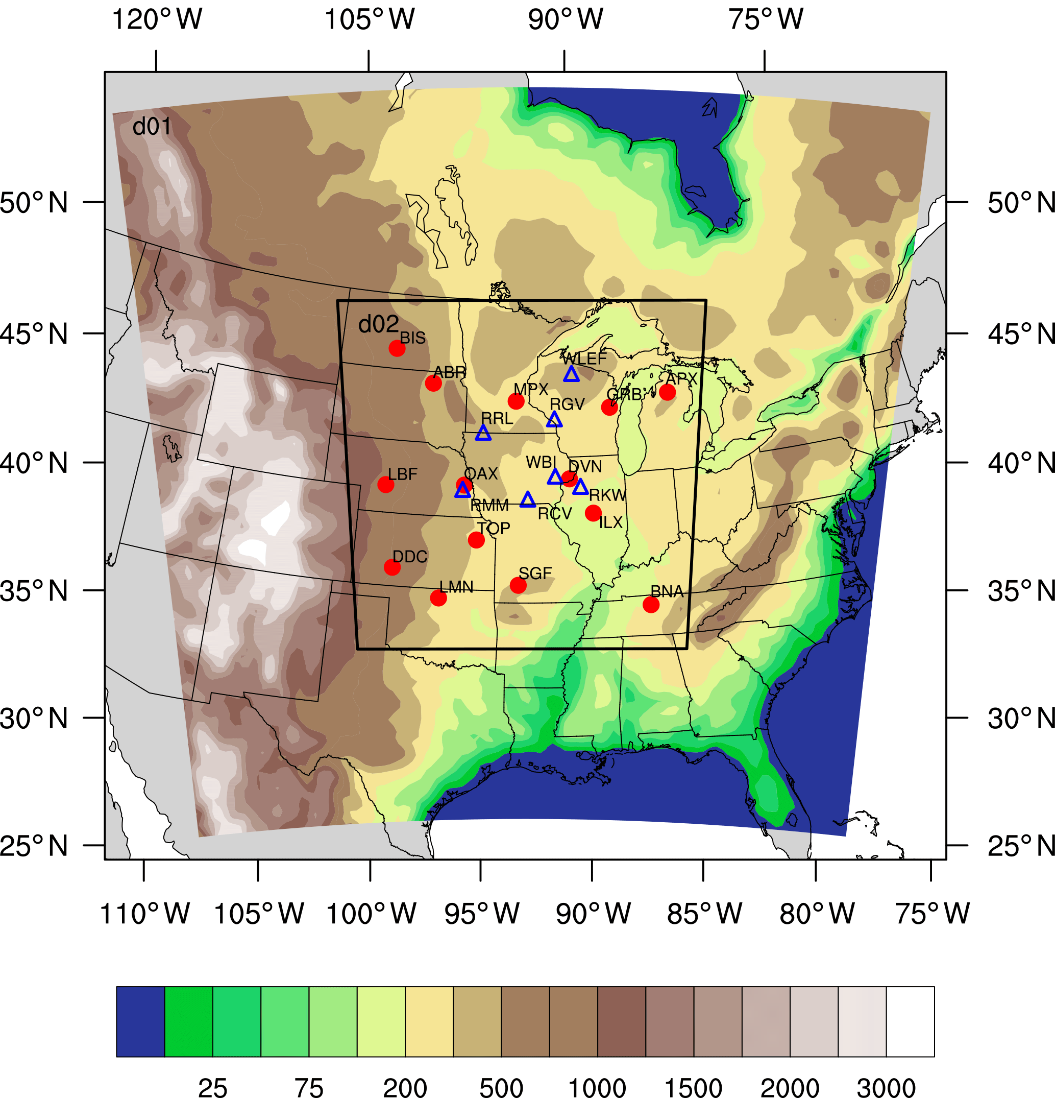
https://www.atmos-chem-phys.net/18/14813/2018/acp-18-14813-2018-f01

Figure 1Geographical domain used by the WRF-ChemCO₂ physics ensemble. The parent domain (d01) is resolved at 30 km in the horizontal; the inner domain (d02) is at 10 km. The color shading represents modeled terrain height in meters above sea level. The inner domain covers the study region and includes the rawinsonde sites (red circles) and the CO₂ tower locations (blue triangles).

Download

2.2 Atmospheric model setup

The atmospheric transport model used in this study to generate our 45-member physics ensemble is the WRF model version 3.5.1 (Skamarock et al., 2008) and a modified chemistry module for CO₂ (called WRF-ChemCO₂; Lauvaux et al., 2012). The atmospheric column in each simulation is described with 59 vertical levels, with 40 of them within the first 4 km of the atmosphere. Two nested domains were used. The coarse domain (d01) uses a horizontal grid spacing of 30 km and the nested or inner domain (d02) uses 10 km grid spacing (Fig. 1). Because of limited computational time and the resolution of the CO₂ surface fluxes described on Sect. 2.6, we decided to keep our highest resolution of the model up to 10 km. The coarse domain covers most of the United States and parts of Canada, and the nested domain is centered over Iowa and covers the Midwest region of United States. The nesting method employed is the “one-way” nesting in which the outer domain constrains the inner domain through nudging of the boundary conditions that drive the meteorology once the outer domain simulation has finished (Soriano et al., 2002). No feedback from the inner domain to the coarse domain was allowed. For our sensitivity study, only the inner domain (d02) has been analyzed as it covers the area of interest.

2.3 Ensemble configuration

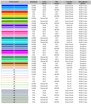
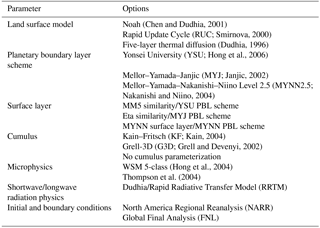
Similar to any domain-limited atmospheric model, transport errors arise from initial and boundary conditions and the different physics parameterizations. Therefore, we have built an ensemble of 45 members using different physical parameterization schemes and large-scale initial and boundary conditions from reanalysis products (see Table 1). WRF offers multiple options for the LSM, PBL, cumulus, and microphysics schemes. The members in our multi-physics ensemble all use the same radiation schemes (both longwave and shortwave) but the land surface, surface layer, boundary layer, cumulus, and microphysics schemes are varied for both the inner and the outer domain. In addition, we have initialized the meteorological boundary and initial conditions with different datasets. Table 2 shows the different options used in this study.

Table 1Different model configurations used in this study.

Download Print Version

2.4 Physics parameterization schemes

2.4.1 Land surface models (LSMs)

The land surface models (LSMs), which ingest land surface properties, soil, and surface conditions from driver data, simulate the conditions at the land surface, including surface energy fluxes. The partitioning of these fluxes affects the structure and depth of the PBL through the turbulence parameterization, hence modifying the near-surface in situ CO₂ mole fractions. To evaluate the sensitivity of modeled mole fractions to the surface conditions, three LSM schemes are chosen for this study: the five-layer soil thermal diffusion model (Dudhia, 1996), the Noah land surface model (Chen and Dudhia, 2001), and the Rapid Update Cycle (RUC) (Smirnova et al., 2000). These LSMs differ in several aspects, from the description of soil properties to the physical processes driving the land–surface interactions. The thermal diffusion model uses a simple thermal diffusion equation to transfer thermal energy from the ground to the atmosphere, describing the belowground profile with five soil layers (Dudhia, 1996). This LSM also includes snow-covered land and constant soil moisture values for a given land use type and season. The Noah LSM scheme uses time-dependent soil temperature and moisture for four soil layers, canopy conductance and moisture, and snow cover prediction (Chen and Dudhia, 2001). The RUC LSM scheme includes six soil layers and includes the effects of vegetation, canopy water, and snow (Smirnova, 2000). This scheme also includes parameterizations for snow and frozen soil (Smirnova, 2000).

Table 2WRF physical parameterizations included in the sensitivity analysis.

Download Print Version | Download XLSX

2.4.2 Planetary boundary layer (PBL) schemes

The planetary boundary layer (PBL) is directly influenced by frictional drag, sensible heat flux, and evapotranspiration, all of which are responsible for generating turbulent eddies. The PBL schemes parameterize turbulent vertical fluxes of heat, momentum, and moisture within the PBL and throughout the atmosphere. The three PBL schemes used in this study are the Yonsei University (YSU) (Hong et al., 2006) PBL scheme, the Mellor–Yamada–Janjic (MYJ) (Janjic, 2002) PBL scheme, and the Mellor–Yamada–Nakanishi–Niino (MYNN) PBL scheme (Nakanishi and Niino, 2004). These three PBL schemes differ in the treatment of turbulent diffusion. The YSU scheme is a first-order scheme that includes non-local eddy diffusivity coefficients to compute turbulent fluxes. The YSU scheme explicitly calculates entrainment at the top of the PBL as a function of the surface buoyancy flux. The MYJ and MYNN 2.5 PBL schemes are local closure schemes that include a prognostic equation for turbulent kinetic energy (TKE) and a level 2.5 turbulence closure approximation to determine eddy transfer coefficients. The MYJ scheme implicitly calculates the entrainment layer while the MYNN uses a more explicit representation of entrainment at the top of the PBL (Román-Cascón et al., 2012). The MYNN 2.5 is a variation of the MYJ PBL scheme that includes a non-local component of the turbulent mixing that reduces potential cold biases and increases PBL depths. The MYJ PBL scheme used in this study has been slightly modified to allow for very low turbulence regimes (e.g., nocturnal stable conditions) with a decreased minimum value for TKE.

2.4.3 Cumulus parameterizations

The cumulus parameterization (CP) schemes are used with the aim of representing the vertical fluxes due to unresolved updraft and downdrafts and compensating motion outside the clouds. In this study, we use two different cumulus parameterization schemes, Kain–Fritsch (KF) (Kain, 2004) and Grell-3D (G3D) (Grell and Devenyi, 2002). The KF scheme is a deep and shallow convection subgrid scheme, which uses a simple cloud model that simulates moist updrafts and downdrafts along with detrainment and entrainment effects. The G3D cumulus scheme is based on the Grell (1993) scheme, and G3D is a scheme for higher-resolution domains allowing for subsidence and neighboring columns. The G3D uses a large ensemble of closure assumptions and parameters that are used in numerical models and implements statistical techniques to determine the optimal value for feedback to the entire model (Pei et al., 2014). The cumulus parameterization is theoretically only valid for coarse grid resolutions (e.g., greater than 10 km) and should not be used when the model has a higher resolution (e.g., less than 5 km) and will resolve cumulus convection (Skamarock et al., 2008). Therefore, we are in a “grey zone” (5–10 km), where it is unclear if cumulus parameterization should be used or not. For that reason, we also ran simulations that do not use a cumulus parameterization scheme in the nested domain.

2.4.4 Microphysics parameterizations

Microphysics parameterizations (MPs) describe cloud and precipitation processes. In this study, we use two MP schemes: the WRF single-moment 5-class (WSM5) scheme (Hong et al., 2004) and the Thompson scheme (Thompson et al., 2004). The WSM5 scheme is a single-moment parameterization that includes five species: water vapor, cloud water, cloud ice, rain, and snow, which are all treated independently. The Thompson scheme is a double-moment scheme, which predicts the mole fraction of five hydrometeors species, the number concentration of ice phase hydrometeors, and rain.

2.5 Meteorological initial and boundary conditions

Two meteorological datasets provide the initial and lateral boundary conditions for our regional model. For initialization, WRF interpolates the coarse-resolution analysis products onto the model grid and calculates the values of the parent domain lateral boundaries. The inner grid uses the boundary conditions of the parent domain. In this study, we compare two different meteorological datasets: the North America Regional Reanalysis (NARR) (Mesinger et al., 2006) and the Final Operational Global Analysis (FNL). The NARR dataset was developed at the Environmental Modeling Center (EMS) of the National Centers for Environmental Prediction (NCEP). NARR uses a high-resolution NCEP Eta model with a horizontal grid spacing of 32 km and includes 45 vertical levels. NARR provides both initial and boundary conditions at 3-hourly intervals. The NCEP FNL analysis data have a horizontal grid spacing of $1^{\circ} \times 1^{\circ}$ and are prepared operationally every 6 h. The FNL is prepared with the same model that NCEP uses in the Global Forecast System (GFS). The initial conditions in the WRF simulations are reset every 5 days to avoid the growth of model errors in the absence of data assimilation. The WRF model spin-up takes about 18 h, so we use model results after 18 h of the first day of each 5-day simulation segment. We compared model–model differences over the 5 days and found no significant trend over the 5-day periods once removing the first 18 h of spin-up.

2.6 CO₂ surface fluxes

For this study, we used the summer 2008 posterior surface fluxes from the data assimilation system CarbonTracker¹ version CT2009 (Peters et al., 2007; with updates documented at https://www.esrl.noaa.gov/gmd/ccgg/carbontracker/, last access: 17 January 2018). This system produces CO₂ flux estimates by integrating daily daytime averaged CO₂ mole fractions from continuous hourly observations and then minimizing the differences between the observed and modeled atmospheric CO₂ mole fractions. The Transport Model 5 (TM5) offline atmospheric tracer transport model (Krol et al., 2005), driven by the European Centre for Medium-Range Weather Forecasts (ECMWF) operational forecast model, propagates the surface fluxes to generate 3-D mole fractions of CO₂ across the globe.

The CO₂ surface fluxes are represented by different subcomponents, which include fossil fuel emissions, biomass burning, terrestrial biosphere exchange, and ocean–atmosphere exchanges. The annual fossil fuel emissions used in CT2009 are from the Carbon Dioxide Information and Analysis Center (CDIAC) (Boden et al., 2009). These fossil fuel fluxes are mapped onto a $1^{\circ} \times 1^{\circ}$ grid and are then distributed into country totals according to the spatial patterns from the EDGAR-4 inventories (Olivier et al., 2001). Biomass burning is based on the Global Fire Emission Database version 2 (GFEDv2). The dataset consists of $1^{\circ} \times 1^{\circ}$ gridded monthly burned areas, fuel loads, combustion completeness, and fire emissions. Prior terrestrial biosphere flux estimates come from the Carnegie–Ames–Stanford approach (CASA) global biogeochemical model (van der Werf et al., 2006; Giglio et al., 2006) with 3 h variability imposed by temperature and incoming radiation (Olsen and Randerson, 2004). The CASA biosphere model produces net primary production (NPP) and heterotrophic respiration fluxes with a monthly time resolution at $0.5^{\circ} \times 0.5^{\circ}$ spatial resolution. The long-term ocean fluxes and uncertainties are derived from inversions reported in Jacobson et al. (2007). Ocean inverse flux estimates are composed of preindustrial (natural), anthropogenic flux inversions, and an additional level of biogeochemical interpretations (Gloor et al., 2003; Gruber et al., 1996). Similar to most CO₂ inverse systems, the fossil fuel and fire emissions are specified (i.e., remain constant) and only the oceanic and terrestrial biosphere fluxes are optimized.

2.7 Dataset

Our interest is to explore and quantify atmospheric transport errors over the US Midwest using observations that we have over this region. Therefore, we will evaluate the errors over the inner domain (d02) of our models. Figure 1 shows the location of all the stations that provide atmospheric CO₂ mole fractions and the meteorological observation sites that will be used. Meteorological data were obtained from the University of Wyoming's online data archive (http://weather.uwyo.edu/upperair/sounding.html, last access: 20 July 2018) for the 14 rawinsonde stations shown in Fig. 1. In situ atmospheric CO₂ mole fraction data are provided by gas analyzers operating continuously on seven communication towers (Fig. 1) (Miles et al., 2012). Five of these towers were part of an experimental network, deployed from 2007 to 2009 (Richardson et al., 2012; Miles et al., 2012, 2013; https://doi.org/10.3334/ORNLDAAC/1202). The other two towers (Park Falls – WLEF and West Branch – WBI) are part of the Earth System Research Laboratory/Global Monitoring Division (ESRL/GMD) tall tower network (Andrews et al., 2014; https://www.esrl.noaa.gov/gmd/ccgg/insitu/, last access: 20 July 2018). Each of these towers sampled air at multiple heights, ranging from 11 to 396 m above ground level (a.g.l.).

2.8 Data selection

Most atmospheric inversions that use continental PBL observations only use daytime CO₂ mole fractions from continuous observations (Law et al., 2003), with the exception of mountain sites whose nighttime data are thought to sample free tropospheric conditions (Brooks et al., 2012). Only daytime measurements are assimilated due to the difficulty in simulating strong vertical gradients in the nocturnal boundary layer. Vertical gradients are minimized during daytime under well-mixed boundary layer conditions (Bakwin et al., 1998). Therefore, both models and observations will be evaluated during daytime.

We analyzed CO₂ mole fractions collected from sampling levels at or above 100 m a.g.l., which is the highest observation level available across the entire MCI network (Miles et al., 2012). This ensures that the observed mole fractions reflect the influence of regional CO₂ fluxes and are minimally influenced by near-surface gradients of CO₂ in the atmospheric surface layer (ASL) due to local CO₂ fluxes (Wang et al., 2007). Both observed and simulated CO₂ mole fractions are averaged from 18:00 to 22:00 UTC (12:00–16:00 LST), the daytime period when the boundary layer should be convective and the CO₂ profile well mixed (e.g., Davis et al., 2003; Stull, 1988). This averaged mole fraction will be referred to hereafter as the daily daytime average (DDA).

In this study, we will also evaluate the PBL wind speed (hereafter wind speed), PBL wind direction (hereafter wind direction), and PBL height (PBLH) from the different rawinsonde stations. Similar to the CO₂ mole fractions, we want our meteorological observations to be within the well-mixed layer. Therefore, we use the wind speed and wind direction observed approximately 300 m a.g.l. CO₂ mole fraction observations were sampled at about 100 m; however, the availability of meteorological observations at this height is too low to collect a sufficient amount of data for our statistical evaluation. The observed PBLH was estimated using the virtual potential temperature gradient with a threshold of 0.2 K m⁻¹. We want our simulated meteorological variables to be close to the observational level; therefore, we use wind speed and wind direction from level 11 (∼350 m) of the model. The WRF model provides an estimate of the PBLH, but the methodology used to diagnose these values varied with the PBL scheme used in the simulation. To remain consistent, we decided to calculate the PBLH in WRF with the same potential temperature gradient method that is used for the rawinsonde data. Rawinsonde stations across this region collect data at 12:00 and 00:00 UTC, but our model–data evaluation will be done for daytime conditions only. Therefore, both the modeled results and data will be evaluated in the late afternoon (i.e., 00:00 UTC) corresponding to well-mixed conditions.

2.9 Evaluation methodology or analyses of the models

Comparisons to measurements of wind speed, wind direction, PBLH, and DDA CO₂ mole fractions are used to inform the performance of each model configuration. Modeled data are extracted from the simulations using the nearest grid points to the locations of our observations. Each model configuration is evaluated from 18 June to 21 July 2008 for the meteorological variables and from 26 June to 22 July 2008 for the CO₂ mole fractions. Summer in the US Midwest corresponds to the peak of the growing season for both crops and most non-agricultural ecosystems (except grasslands). We focus here on the growing season because the large biogenic fluxes make this period the most important time of year for understanding the relationship between fluxes and CO₂ mole fractions. We first explore meteorological variables, and the sensitivity of CO₂ to atmospheric transport but without comparison to observations, to avoid confounding the impact of transport with errors from CO₂ surface fluxes and CT2009 global CO₂ mole fractions. Finally, we compare CO₂ observations with the knowledge that the results include both transport and CO₂ flux errors.

2.9.1 Analyses of physics parameterization and reanalyses impact

The daily mean of root mean square difference (RMSD) among ensemble members is used to isolate the atmospheric transport variability and evaluate the impact of the physics parameterizations on both CO₂ mole fractions and PBL dynamics. The RMSD does not consider the observations as we take the square root of the average difference between model configuration and the ensemble mean:

\begin{matrix} (1) & \overline{RMSD} = \sum_{i = 1}^{N} \frac{\sqrt{\frac{1}{n} \sum_{j = 1}^{n} {(p_{j i} - μ_{i})}^{2}}}{N}, \end{matrix}

where p_ji is the predicted variable for ensemble member j and day i, μ_i is the mean of the ensemble for day i, N is the total number of days, and n is the number of members. The RMSD was estimated for the different physics parameterization used (i.e., LSM, PBL schemes, CP, MP) and reanalysis. A different set of ensembles were created for each of the physics parameterization, where the model configuration remained identical except for the tested physics parameterization, and the different set of members was used to compute the ensemble mean. The RMSD of the simulated CO₂ mole fractions was used to explore if other physics parameterizations have a significant impact on CO₂ mole fractions compared to the PBL parameterizations. To explore which parameterizations impact the PBL dynamics, we applied the RMSD to the three selected meteorological variables (i.e., PBLH, wind speed, and wind direction), assuming these variables contribute the most to the representations of the CO₂ mole fraction distributions in the PBL. The RMSDs for the meteorological variables were then averaged across all of the rawinsonde sites. The RMSD of the CO₂ mole fractions was estimated using the simulated CO₂ mole fraction at each communication tower and then averaged across the tower sites to match the model–data residual.

2.9.2 Analyses of model–data residuals

A series of statistical analyses are used to assess the performance of the different model configurations for the three meteorological variables' wind speed, wind direction, and PBLH. The different metrics used include the root mean square error (RMSE) and mean bias errors (MBE):

\begin{array}{l} (2) & RMSE = \sqrt{\frac{1}{N} \sum_{i = 1}^{N} {(p_{i} - o_{i})}^{2}}, \\ (3) & MBE = \frac{1}{N} \sum_{i = 1}^{N} (p_{i} - o_{i}), \end{array}

where o_i is the observed variable for day i, p_i is the predicted variable for day i, and N is the total number of days. The RMSE represents the magnitude of the model error without regard to the long-term mean (Wilks, 2011). The MBE describes the model–observations difference averaged errors over the entire period (Wilks, 2011), and identifies model bias. These two metrics are critical to inverse flux estimates as biases can arise from day-to-day (which we will refer as random) or longer-term (systematic) errors in the transport model. We acknowledge that the propagation of meteorological errors to mole fractions, and mole fraction errors to surface fluxes, is complex, but these metrics provide valuable insight into model performance. Each of these statistics (i.e., RMSE and MBE) was estimated for each model and each rawinsonde site using the late afternoon (00:00 UTC) soundings.

Finally, we compare modeled and simulated PBL CO₂. We use our different model configurations, which all share the exact same surface fluxes and identical boundary conditions to explore the impact of the transport errors on CO₂ mole fractions. We present the impact of model configurations on the DDA CO₂ mole fraction model–data mismatches (or residuals) with Taylor diagrams and correlation between model–data residuals in meteorological variables and DDA CO₂ mole fractions. The Taylor diagram relies on three nondimensional statistics: the variance ratio (model variance normalized by the observed variance), the correlation coefficient, and the normalized centered root mean square (CRMS) difference (Taylor, 2001). The variance ratio or normalized standard deviation (NSD) indicates the difference in amplitude between the model and the observation. If this ratio is less than 1.0, then the model tends to underestimate the amplitude compared to the observation. The correlation coefficient measures the similarity in the temporal variations between the model and the observation, regardless of the amplitude. This correlation coefficient has a range of $- 1.0 \leq R \leq 1.0$ and is insensitive to systematic errors. As R approaches 1.0, the model approaches agreement with the observation. The CRMS is normalized by the observed standard deviation and quantifies the ratio of the amplitude of the variations between the model and the observation. The CRMS is also insensitive to systematic errors. Temporal correlations between the modeled–observed residual in meteorological variables and CO₂ mole fractions are used to determine the impact that meteorological errors have on the PBL CO₂ mole fractions. This model–data correlation will be done between each CO₂ observing site and rawinsonde site; therefore, we will be able to observe if any correlation is dependent on the distance between sites. The model–data residual includes both flux and transport errors; therefore, these errors will not show the accuracy of the transport model. Nevertheless, each simulation uses the same CO₂ flux and boundary conditions that allow us to use the model–data residuals as an indicator of the differences between model configurations.

3 Results

3.1 Impact of physics parameterizations on atmospheric CO₂ mole fractions

The daily mean of RMSD of the simulated CO₂ mole fraction was used to explore the sensitivity of CO₂ mole fractions to model physics parameterization and meteorological reanalysis. The RMSD was computed for different parameterizations schemes (i.e., LSM, PBL, CP, and MP) and for two reanalysis products (i.e., NARR and FNL). For each group of parameterizations, the model configuration remained identical except for the tested parameterization scheme. For example, to evaluate the impact of LSM schemes on CO₂ mole fractions, three LSM schemes were used while preserving the exact same physical schemes for the PBL, CP, MP, and the reanalysis data. Figure 2 shows the results of these experiments. CO₂ mole fraction RMSD is greatest for the LSM, followed by the PBL scheme and CP. The microphysics parameterization has the least impact on CO₂ mole fractions. Only two microphysics parameterizations are tested in this ensemble but additional tests using only two options for all the different physic parameterizations produced similar results.

We also explore how much the variability in PBL winds and depth is influenced by physics parameterizations. Figure 3 shows the RMSD of PBL wind speed and direction, and PBLH over the entire simulation period. The results for all three meteorological variables are similar to those for CO₂ mole fractions. Reanalysis has a greater impact on wind speed (Fig. 3b) and wind direction (Fig. 3c) than it does on PBLH (Fig. 3a). It is worth noting that the PBLH RMSD (Fig. 3a) shows the same RMSD ranking (i.e., relative importance of the physics) as for CO₂ mole fraction RMSD (Fig. 2).

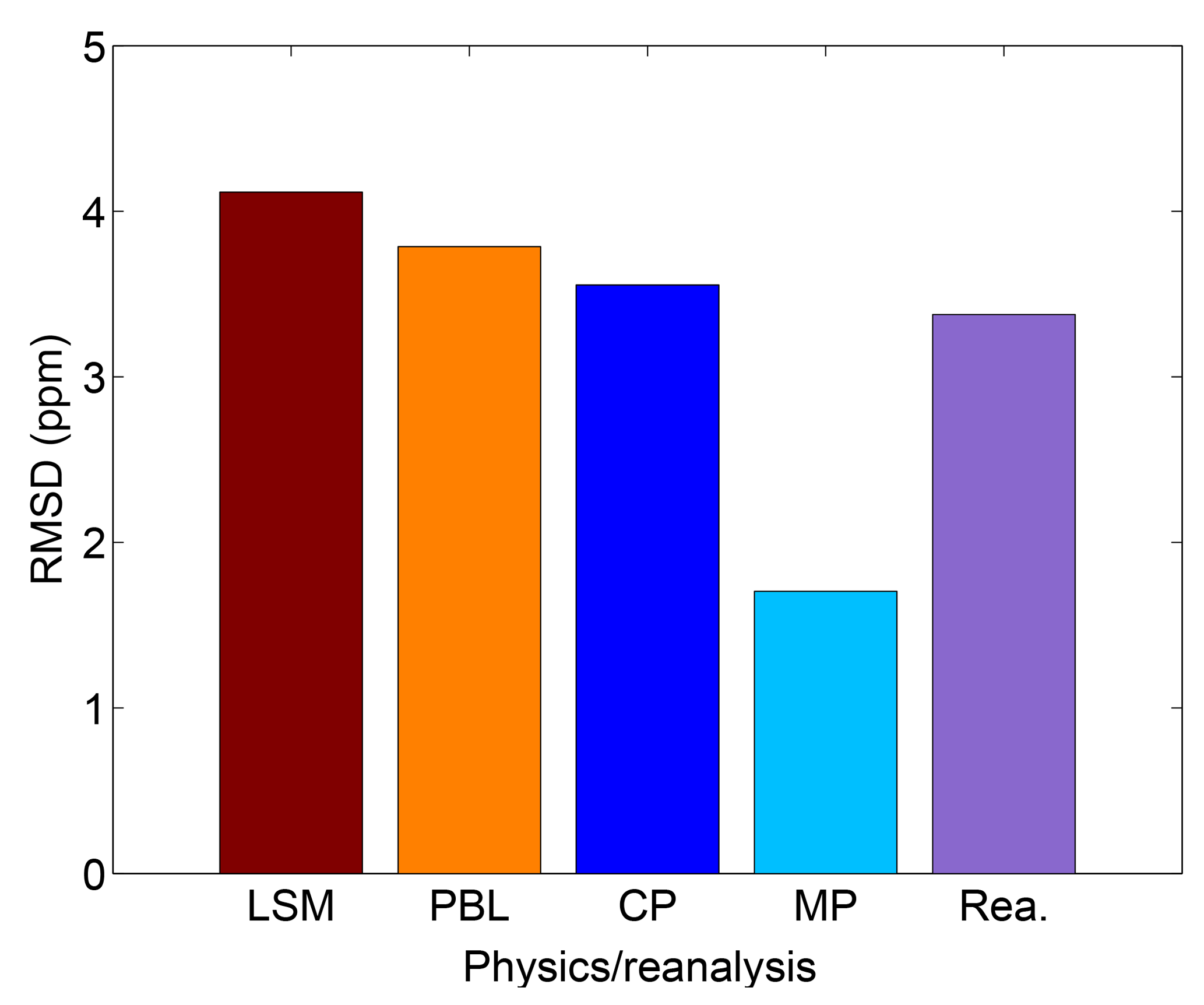
https://www.atmos-chem-phys.net/18/14813/2018/acp-18-14813-2018-f02

Figure 2Sensitivity of CO₂ mole fractions as a function of model physics parameterizations, i.e., land surface model (LSM), planetary boundary layer scheme (PBL), cumulus parameterization (CP), microphysics parameterization (MP) and reanalyses. The root mean square difference (RMSD) of the CO₂ mole fractions simulated at each site and for each model ensemble member was computed by varying only the type of physics parameterization noted and keeping all other model elements constant. RMSD was averaged across sites and across model ensembles.

Download

Based on the evaluation of the CO₂ mole fraction, wind speed, wind direction, and PBLH RMSD, the LSM has the greatest impact on PBL CO₂ transport, followed closely by the PBL scheme, CP, and reanalysis. All the parameterization schemes, including the reanalysis data source, have a significant impact on each of these variables. The RMSDs were significant values compared to typical spatial and temporal differences (for PBL CO₂; see Miles et al., 2012) and for mean PBL properties (PBLH, winds), confirming the importance of model parameterization for these variables.

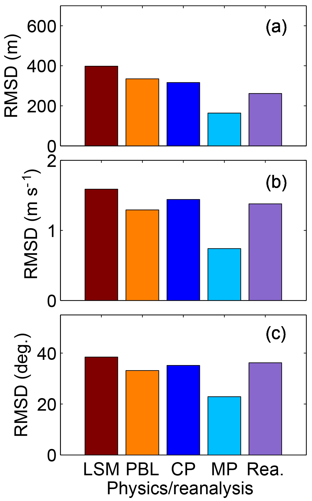
https://www.atmos-chem-phys.net/18/14813/2018/acp-18-14813-2018-f03

Figure 3Root mean square difference (RMSD) of the PBLH (a), wind speed (b), and wind direction (c) for the different physics parameterizations, i.e., land surface model (LSM), planetary boundary layer scheme (PBL), cumulus parameterization (CP), microphysics parameterization (MP) and reanalyses. The RMSDs were computed in the same way for these variables as for PBL CO₂ in Fig. 2.

Download

3.2 Meteorological day-to-day variability

Figure 4 shows a time series of the 00:00 UTC observed and simulated wind speed (Fig. 4a), wind direction (Fig. 4b), and PBLH (Fig. 4c) from 18 June to 21 July 2008 at the Chanhassen, Minnesota (MPX), rawinsonde site. Across the study region, we found maximum monthly average model–data differences across sites and configurations of 9 m s⁻¹ for wind speed, 153^∘ in wind direction, and 2000 m for PBLH. These values confirm the large spread among model results and sites over the simulation time period. Other sites have similar characteristics to Fig. 4. The ensemble shows less variability (i.e., relative spread of the ensemble compared to the observed variability) for the wind speed and wind direction compared to the PBLH. The time series at each rawinsonde site shows that for certain days, all ensemble are biased (i.e., all the members either overestimate or underestimate) as compared to observed wind speed and wind direction (e.g., DOYs 181 and 201, respectively). The time series of the PBLH, however, shows that simulated PBLH can vary significantly across the different physics configurations and that the ensemble encompasses the observed PBLH over the time period.

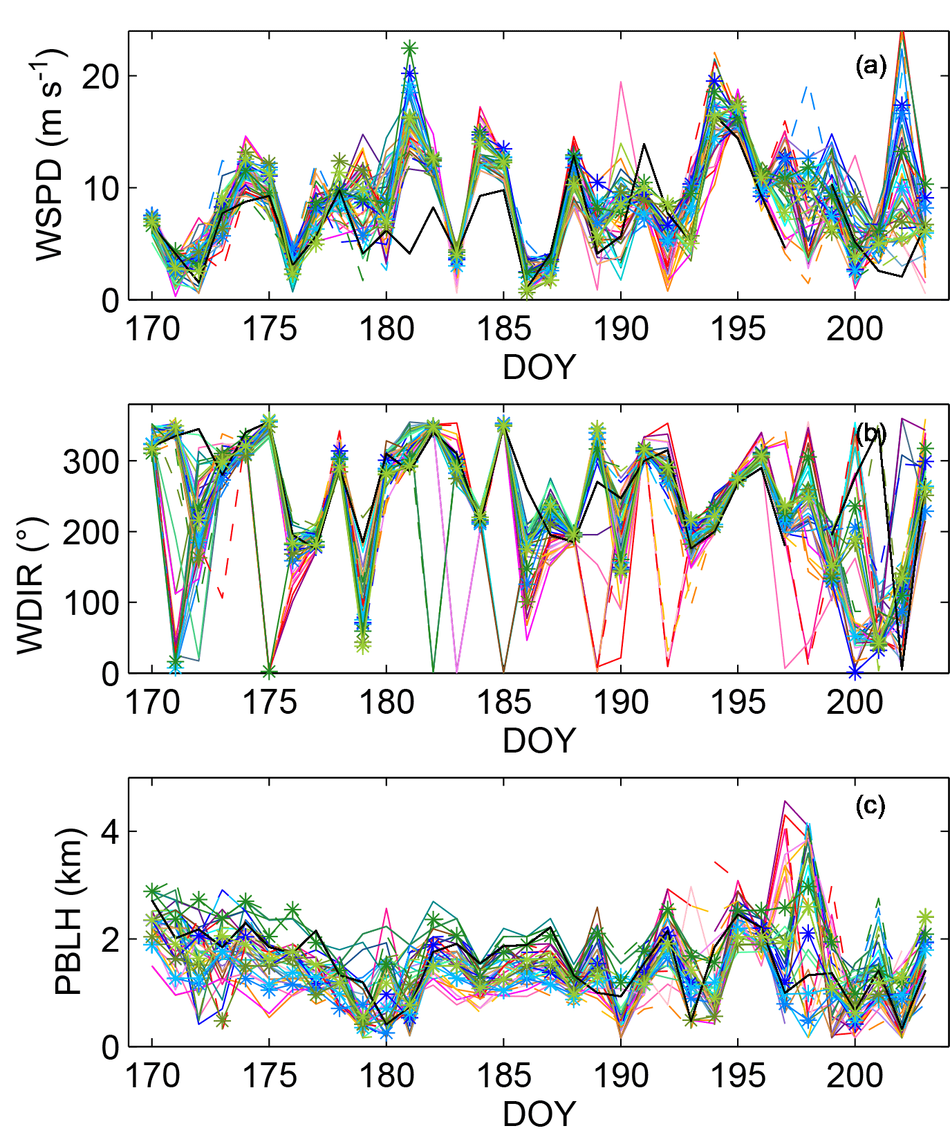
https://www.atmos-chem-phys.net/18/14813/2018/acp-18-14813-2018-f04

Figure 4Observed (black line) and simulated (colored lines; see Table 1) PBL (300 m a.g.l.) wind speed (a), wind direction (b), and PBLH (c) at 00:00 UTC from day of the year (DOY) 169 to 203 of 2008 at the Chanhassen, Minnesota (MPX), rawinsonde site.

Download

3.3 Characterization of transport errors

3.3.1 Root mean square error (RMSE)

Figure 5 shows the regionally and monthly averaged RMSE of wind speed (Fig. 5a), wind direction (Fig. 5b), and PBLH (Fig. 5c) for the different model configurations. For both wind speed and wind direction, we found small to no differences in the regional RMSE as a function of model configuration. Although the regional RMSEs for both wind speed and wind direction are fairly constant, the two variables have the same two model configurations with the highest RMSE. These two configurations share the same LSM scheme (RUC) and the same PBL scheme (MYJ) (models 14 and 23; see Fig. 5a, b and Table 1). Differences among configurations are larger in the regional RMSE of the PBLH (Fig. 5c), with configuration RMSEs ranging from 680 to 1149 m. The model configurations that show the highest PBLH RMSEs include the same LSM (RUC) and PBL parameterization scheme (YSU) (models 4, 13, 22, and 34; see Fig. 5c and Table 1). Although the configurations that show the highest RMSEs are not always the same across the different variables, these configurations share the same LSM (RUC). The two model configurations that showed the lowest RMSE for both wind speed and wind direction both used MYNN 2.5 as their PBL parameterization. Many configurations show low RMSE for the PBLH and all the configurations with low RMSE use either the MYJ scheme or the MYNN 2.5 scheme. However, no single configuration performs best at the regional scale for all of the meteorological variables.

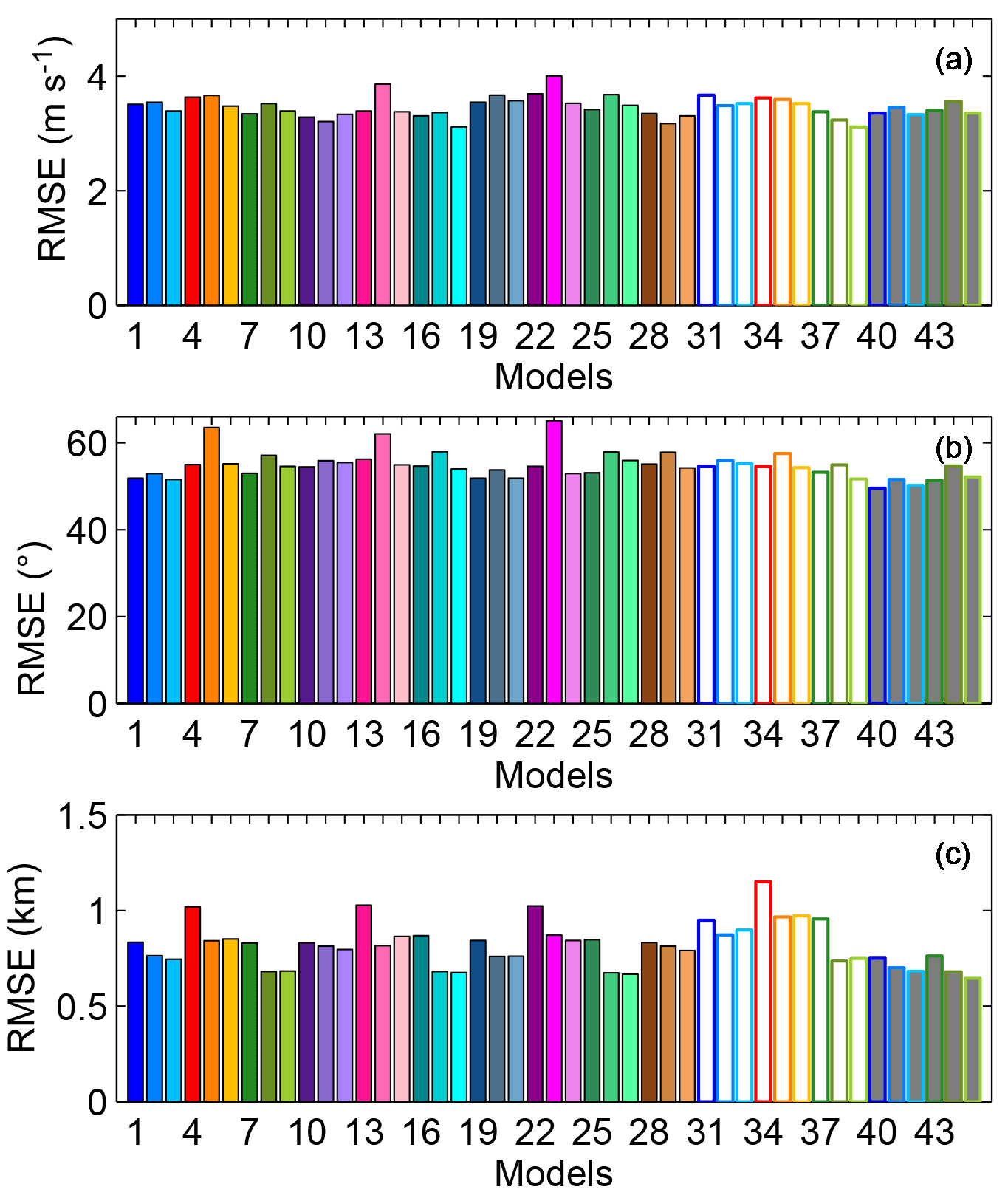
https://www.atmos-chem-phys.net/18/14813/2018/acp-18-14813-2018-f05

Figure 5Regional averages of the monthly average of wind speed (a), wind direction (b), and PBLH (c) RMSE for the different models (see Table 1 for model configurations).

Download

https://www.atmos-chem-phys.net/18/14813/2018/acp-18-14813-2018-f06

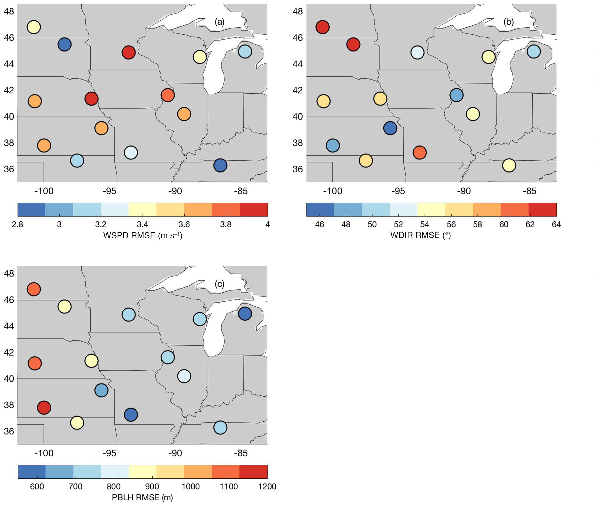
Figure 6Ensemble mean of monthly averaged RMSE of wind speed (a), wind direction (b), and PBLH (c).

Download

We computed the ensemble mean of the monthly averaged RMSE at each of the rawinsonde sites for wind speed (Fig. 6a), wind direction (Fig. 6b), and PBLH (Fig. 6c). We did not find any regional patterns in wind speed (Fig. 6a) and wind direction (Fig. 6b). However, PBLH shows that the highest RMSEs are located in the west of the domain, with an RMSE 400 m or higher than the sites in the east.

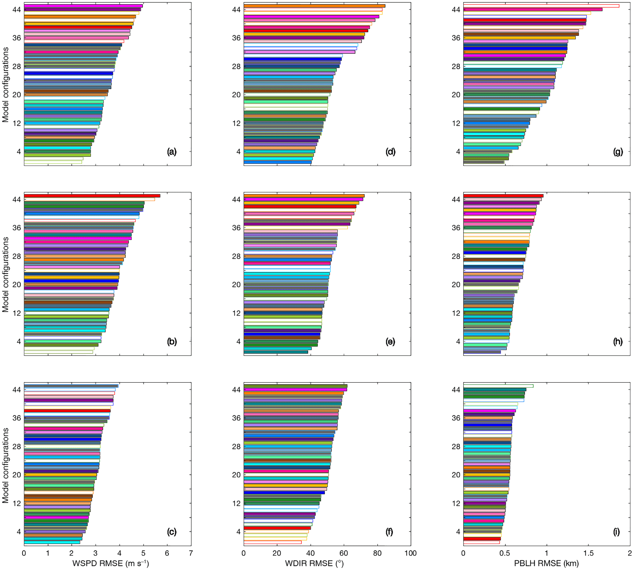
https://www.atmos-chem-phys.net/18/14813/2018/acp-18-14813-2018-f07

Figure 7Monthly average wind speed (a–c), wind direction (d–f), and PBLH (g–i) RMSE for rawinsonde sites North Platte Regional Airport, Nebraska (LBF) (first row), MPX (second row), and Gaylord, Michigan (APX) (third row). Models are sorted from the smallest to the highest RMSE. Model configurations are ordered by RMSE and identified by color (see Table 1).

Download

Figure 7 shows the monthly average RMSE of wind speed (Fig. 7a–c), wind direction (Fig. 7d–f), and PBLH (Fig. 7g–i) for each model configuration at specific rawinsonde sites. We computed the RMSE for all the different sites (not shown), and we found the highest RMSE in the model configurations that included RUC and thermal diffusion as the LSM and at some sites when these LSMs were combined with YSU as a PBL scheme. Although the RMSE was computed at each of the rawinsonde sites, we show only three sites located in three different regions of the domain: North Platte Regional Airport, Nebraska (LBF), in the west (Fig. 7a, d, g), MPX, which is close to the center of the domain (Fig. 7b, e, h), and Gaylord, Michigan (APX) (third row), in the eastern part of the domain (Fig. 7c, f, i). Similar to the regional RMSE (Fig. 5), both LBF and MPX show that the LSM RUC leads to the highest RMSE for the three meteorological variables. However, this pattern is not found at APX, where other configurations show the highest RMSE for wind speed, wind direction, and PBL height. Across simulations and meteorological variables, RMSEs vary, but no configuration shows a lower value across all sites.

3.3.2 Mean bias error (MBE)

The average over- or underestimation of the model configurations is assessed by computing the regional monthly average MBE for wind speed (Fig. 8a), wind direction (Fig. 8b), and PBLH (Fig. 8c). In this study, a positive MBE means the model configuration is systematically higher than the observation. We found remarkable variations in the regional MBE both as a functions of different model configurations and across the meteorological variables. The regionally averaged PBL wind speed bias for any single ensemble member ranges from −0.2 to 1.2 m s⁻¹, relative to the mean regional midday wind speed of 6.2 m s⁻¹, showing that the bias of any single ensemble member ranges from less than 5 % to nearly 20 % of the regional mean PBL wind speed (Fig. 8a). All configurations that use YSU (e.g., models 1, 4, 7, 10; see Fig. 8a and Table 1) have greater regional wind speed biases than the rest of the PBL schemes. The regional MBE for wind direction varies according to model configuration. Models using YSU as PBL schemes tend to show a systematic positive bias in the wind direction (e.g., models 1, 4, 7, 10; see Fig. 8b and Table 1), whereas models that use MYJ as PBL scheme show a negative bias (e.g., models 2, 5, 8, and 11; Fig. 8b and Table 1). Similar to the wind direction, the regional PBLH bias is correlated with model configuration. Any model configuration that uses YSU shows a positive bias, larger than the rest of the PBL schemes (e.g., models 1, 4, 7, 11; see Fig. 8c and Table 1). The model configurations that do not include cumulus parameterizations (white filled bars; Fig. 8c) also show positive biases, with one exception, regardless of the choice of LSM or PBL scheme used. The wind speed analysis shows that the two model configurations with the smallest regional MBE (±0.1 m s⁻¹) share the same LSM (thermal diffusion) and PBL (MYNN 2.5) parameterization. For wind direction, two of the three model configurations with the lowest MBE (±0.1^∘) use the same LSM (Noah) and PBL (YSU) parameterizations. All 15 model configurations with the lowest MBE for PBLH (±100 m or less) share the same PBL parameterizations (MYJ and MYNN 2.5). Although the configurations that provide the lowest regional MBE are not the same across all variables, we found that the lowest biases for the three variables were produced by model 18 (see Table 1). This model configuration is driven by the NARR reanalysis product and used thermal diffusion as the LSM, MYNN as the PBL scheme, Grell-3D as the CP, and WSM 5-class as the MP.

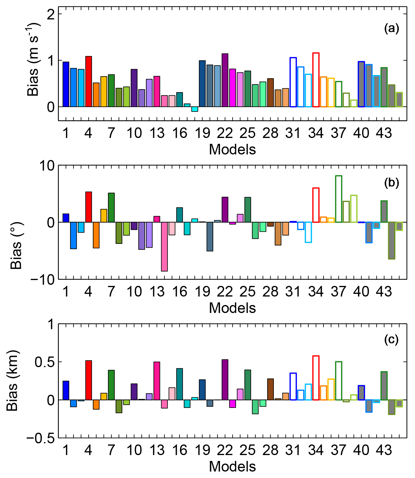
https://www.atmos-chem-phys.net/18/14813/2018/acp-18-14813-2018-f08

Figure 8Regional average of the monthly average of PBL wind speed (a), PBL wind direction (b), and PBLH (c) bias for the different model configurations (identified by number and color; see Table 1).

Download

https://www.atmos-chem-phys.net/18/14813/2018/acp-18-14813-2018-f09

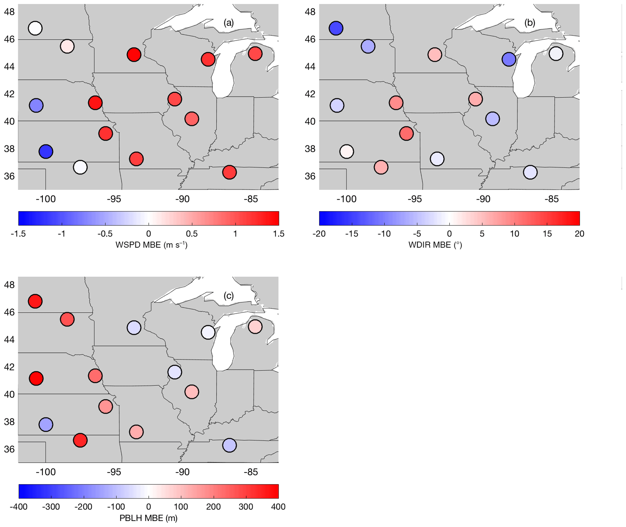
Figure 9Ensemble mean of the mean bias error (MBE) for PBL wind speed (a), PBL wind direction (b), and PBLH (c).

Download

The spatial structures of the MBE over a month are evaluated by estimating the ensemble mean of the MBE at each rawinsonde site (Fig. 9). The ensemble mean of the MBE reveals a spatial pattern in the wind speed (Fig. 9a) and PBLH (Fig. 9c). The map of wind speed MBE (Fig. 9a) shows that the ensemble is positively biased in the eastern region of the domain. However, sites in the western region of the domain show that the ensemble average has either negative or near-zero wind speed MBEs. The PBLH MBE map (Fig. 9c) also shows a clear spatial pattern, with the highest values, nearly all positive, at sites located in the western part of the domain, whereas the sites in the eastern part of our domain show a smaller MBE and no distinct regional sign. PBL wind direction does not show any spatial pattern in the ensemble mean of the MBE (Fig. 9b). We found that our ensemble of simulations can produce an MBE range from rawinsonde site to rawinsonde site of ±1.5 m s⁻¹ in wind speed, ±20^∘ for wind direction, and ±400 m for PBLH.

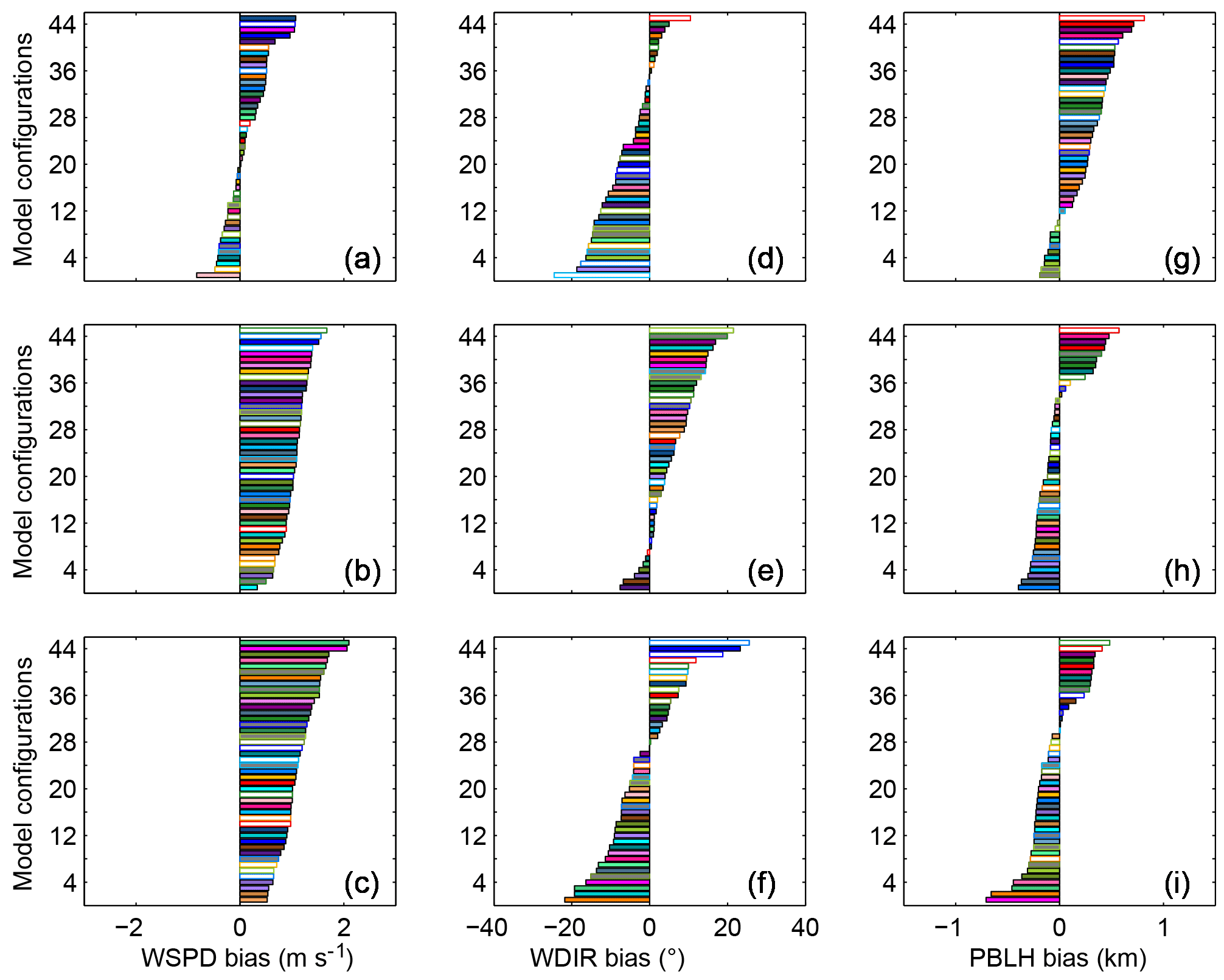
https://www.atmos-chem-phys.net/18/14813/2018/acp-18-14813-2018-f10

Figure 10Monthly average wind speed (a–c), wind direction (d–f), and PBLH (g–i) MBE for rawinsonde sites Aberdeen, South Dakota (ABR) (first row), Davenport, Iowa (DVN) (second row), and Nashville Airport, Tennessee (BNA) (third row). Models are sorted from negative to positive bias. Model configurations are ordered by MBE and identified by color (see Table 1).

Download

The MBE analysis was performed for all the sites (not shown); for this statistic, we found that all the model configurations show a positive wind speed MBE (overestimation) for the majority of the rawinsonde sites, whereas wind direction and PBLH show both positive and negative (underestimation) MBEs across the different configurations at the different rawinsonde sites. Some of the positive and negative biases are associated with specific LSMs and PBL schemes. Figure 10 shows the MBEs of three sites that are representative of regional patterns. The three sites shown are located in three different regions of the domain: Aberdeen, South Dakota (ABR), in the west (Fig. 10a, d, g), Davenport, Iowa (DVN), which is close to the center of the domain (Fig. 10b, e, h), and Nashville Airport, Tennessee (BNA), in the eastern part of the domain (Fig. 10c, f, i). Most of the model configurations show positive wind speed MBE (overestimation) for the majority of the rawinsonde sites (e.g., Fig. 10b–c); however, one site shows both positive and negative MBEs for the different model configurations (e.g., Fig. 10a). Overall, we found that 10 out of the 14 rawinsonde sites show all the model configurations with a positive wind speed bias; these sites were located in the eastern and center areas of the domain. However, the MBEs for wind direction (e.g., Fig. 10d–f) and PBLH (e.g., Fig. 10g–i) are highly variable across the rawinsonde sites. At the majority of the sites, the simulations had both positive and negative biases. Although wind speed and wind direction do not show any of the simulations with a systematic behavior across the sites, PBLH MBE showed some simulations with systematic bias across the different sites. The highest positive biases were found in configurations that use RUC as the LSM and YSU as the PBL scheme in the western region of the domain (e.g., Fig. 10g, red bars). This is unlike the eastern region of the domain, where the highest biases were dominated by configurations that use thermal diffusion as the LSM and YSU as the PBL scheme (e.g., Fig. 10i, white bar with green border). These results indicate that wind speed MBEs are strongly impacted by other components of the model (e.g., reanalysis dataset) or that the WRF transport model carries a systematic bias that will show up regardless of the configuration used. However, PBLH bias is highly controlled by two components of the model, the LSM and the PBL parameterization scheme. Overall, the spatial patterns show that no configurations can avoid spatial biases across the region.

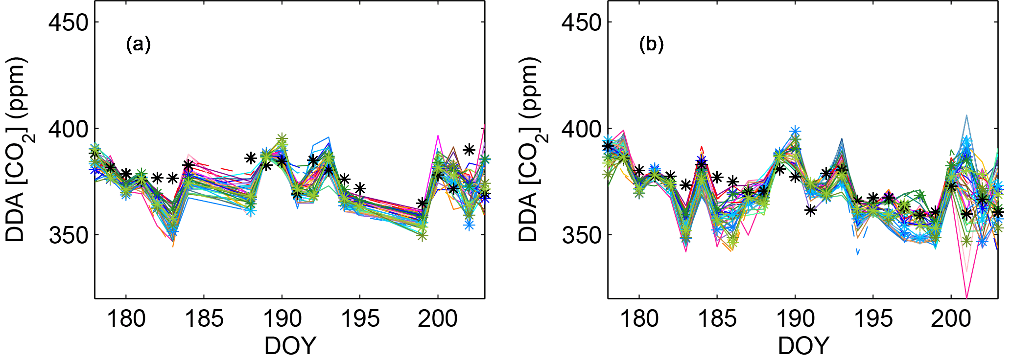
https://www.atmos-chem-phys.net/18/14813/2018/acp-18-14813-2018-f11

Figure 11Observed (black stars) and simulated (colored lines) DDA CO₂ mole fraction (ppm) at Centerville (RCV) (a) and WBI (b).

Download

3.4 Sensitivity of CO₂ mole fractions to model configuration

Figure 11 shows simulated and observed atmospheric DDA CO₂ mole fraction for Centerville (Fig. 11a) and Kewanee (Fig. 11b) from 26 June to 21 July 2008. For this period, both sites show large residuals that are not encompassed by the ensemble spread (RMSD) for several periods (e.g., DOYs 182–183 at Centerville or DOYs 185–186 at WBI). This result suggests that transport model errors from our ensemble only represent a fraction of the total uncertainty in our modeling system. In this study, we use CarbonTracker fluxes which is a global inversion system and does not aim to represent regional fluxes. Therefore, additional errors can be due to incorrect CO₂ surface fluxes and boundary conditions.

Over the region, most of the sites show that the ensemble generally underestimates the atmospheric CO₂ mole. We note here that this ensemble has not been calibrated; therefore, the ensemble spread is unlikely to serve as quantification of WRF transport errors or total error in simulated PBL CO₂, but this sensitivity test could have resulted in an ensemble spread that is much larger than the model–data differences. Our results suggest that the spread of this physics ensemble underestimates total model–data error in PBL CO₂.

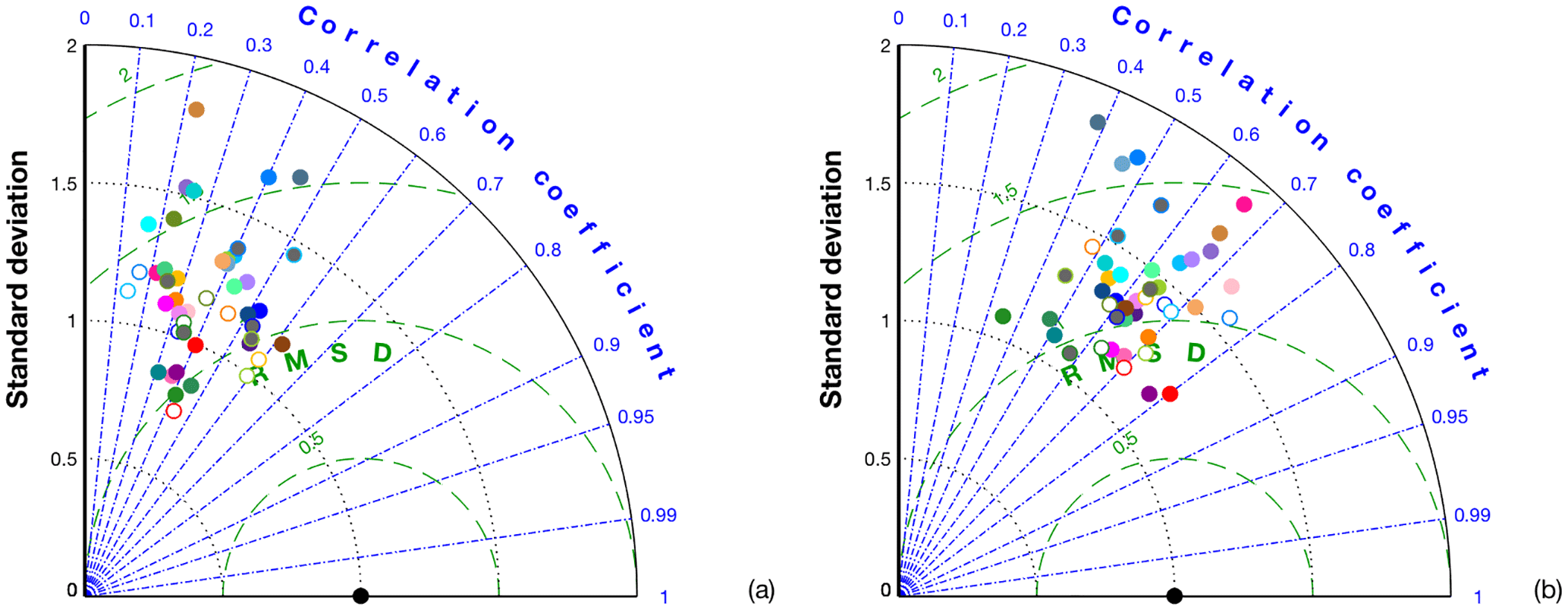
https://www.atmos-chem-phys.net/18/14813/2018/acp-18-14813-2018-f12

Figure 12Taylor diagram comparing observations versus simulations at (a) Mead (RMM) and (b) West Branch (WBI), using DDA CO₂ mole fractions from 100 m a.g.l. Black dots at (1, 1) represent the observations.

Download

To evaluate the performance of the different models over the month, we computed the correlation coefficient, the NSD and the CRMS difference (Taylor, 2001) for each of the in situ sites. These results are presented as Taylor diagrams (Fig. 12) using the DDA observed and simulated CO₂ mole fractions. Nearly all ensemble members overestimate the temporal variability at in PBL CO₂ (e.g., Fig. 12a) and at some sites all members overestimate the temporal variability (e.g., Fig. 12b). The correlation between simulated and observed CO₂ mole fractions can vary from 0.8 to 0.1, indicating a wide range of model performance at site level. Interestingly, some of the models that show a high correlation between the modeled and observed DDA CO₂ mole fractions are the model configurations with the highest PBLH bias (see Fig. 8c, models 4 and 22).

The correlation between meteorological and CO₂ mole fraction model–data differences is evaluated using the MBE for each model at the different rawinsonde and CO₂ tower sites. These correlations (Fig. 13) reveal that, to first order, errors in simulated PBLH govern model–data differences in PBL CO₂ mole fraction. Both wind speed (Fig. 13a) and wind direction (Fig. 13b) show low correlations, whereas PBLH (Fig. 13c) shows consistently positive correlation with the CO₂ mole fraction errors across all sites. We did not find any relationship between error correlation and distance (see Fig. A1 in Appendix). These results suggest that the bias errors in the in situ CO₂ mole fractions are directly related to the MBE in PBLH. The sign of the correlation (overpredicted PBLH correlated with overpredicted PBL CO₂) is expected given net uptake of CO₂ by the regional biosphere.

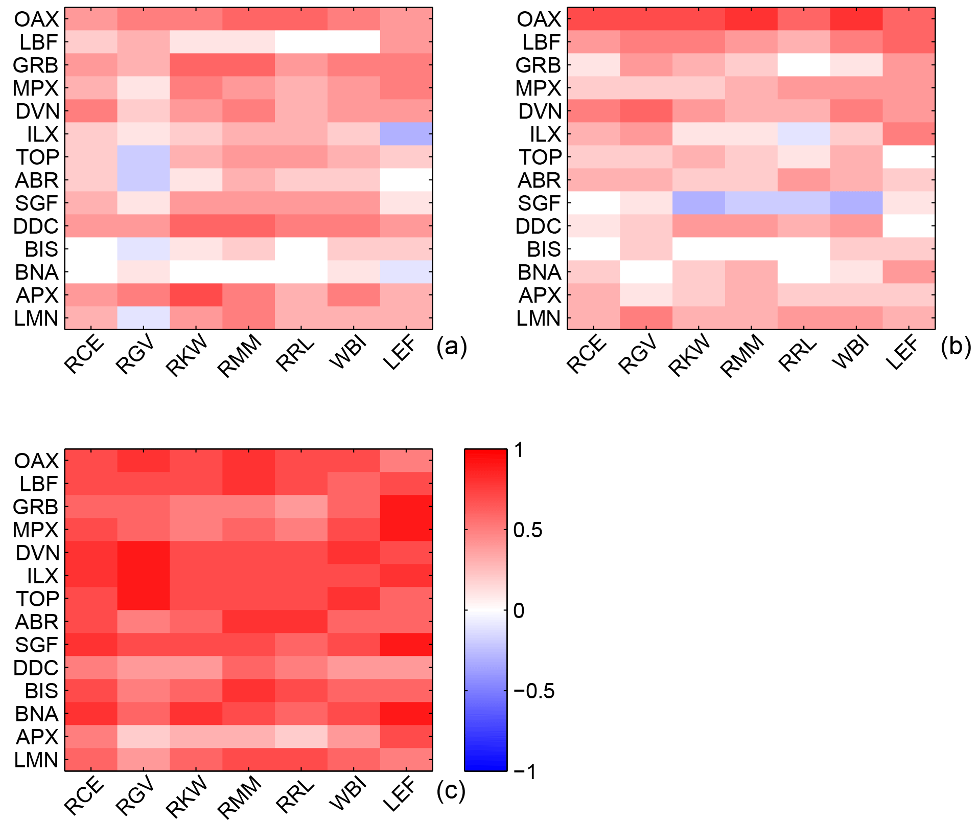
https://www.atmos-chem-phys.net/18/14813/2018/acp-18-14813-2018-f13

Figure 13Tower and rawinsonde site-specific spatial correlation coefficients between ensemble mean MBE of (a) wind speed, (b) wind direction and (c) PBLH and ensemble mean MBE of DDA CO₂ mole fractions. The abscissa shows the different CO₂ tower sites, while the ordinate shows rawinsonde sites.

Download

4 Discussion

The evaluation of the RMSD of daytime PBL CO₂ mole fractions shows that all the physics parameterizations have a significant impact on the simulated values, with only the microphysics parameterization showing a lesser impact (Fig. 2). Previous research has focused on the potential impact of PBL schemes on CO₂ mole fractions (e.g., Kretschmer et al., 2012, 2014; Lauvaux and Davis, 2014). Results from our study indicate that other physics parameterizations including the LSM and CP generate errors of similar magnitude in simulated daytime PBL CO₂ mole fractions (Fig. 2). The PBLH is also sensitive to all of these physical parameterizations (Fig. 3a), and there is a high correlation between PBLH errors and CO₂ mole fraction errors (see Fig. 13c). In this sense, our results agree with previous research that assumes that the misrepresentation of the PBLH plays an important role in PBL CO₂ errors (Stephens et al., 2007; Gerbig et al., 2008; Kretschmer et al., 2012). We show, however, that multiple elements of the modeling system, not just the PBL parameterization, influence PBLH. Further, although PBL wind speed (Fig. 13a) and wind direction (Fig. 13b) errors are not clearly correlated with PBL CO₂ errors, this does not imply that these errors are unimportant. Figure 2 also shows that the reanalysis has an impact on atmospheric CO₂ mole fractions, which indicates that even if the wind speed and wind direction errors do not show a high correlation with atmospheric CO₂ errors (Fig. 13a–b), these two variables can contribute to the errors in CO₂ mole fractions. Indirectly, we demonstrated that the reanalysis directly impacts CO₂ mole fractions by changing wind speed and direction in WRF (Fig. 3b–c), whereas PBLH errors are primarily driven by physical schemes (surface and PBL schemes). The relationship between PBL winds and CO₂ mole fraction is dependent on the local spatial distribution of CO₂ surface fluxes and could easily show no clear correlation when averaged over time and space. However, we know errors in these two variables can impact the distribution and magnitude of the inverse CO₂ fluxes over the region (Deng et al., 2017; Lauvaux and Davis, 2014).

The square root of the model errors (RMSE) of wind speed and wind direction shows similar magnitudes in the errors regardless of the model configuration that we use. Additionally, we found over the region a systematic positive bias (MBE; overestimation) of wind speed for the majority of the model and sites. These results, especially the ones from wind speed, lead us to consider other elements of the models as a contributor of the errors. Past literature has stated and shown that the WRF mesoscale model has a tendency to produce high wind speed over land (Cheng and Steenburgh, 2005; Roux et al., 2009; Zhang et al., 2009; Yerramilli et al., 2010; Jimenez and Dudhia, 2012). Some studies have attributed this high wind speed bias to the smoothed representation of the topography (Jimenez and Dudhia, 2012; Santos-Alamillos et al., 2013). Biases of approximately 3 m s⁻¹ have been attributed to this misrepresentation of topography. Fovell and Cao (2014) argue that the misrepresentation of the terrain, or possibly the vegetation, can produce a biased roughness length that can lead to wind speed biases of about 2 m s⁻¹. There are other factors that contribute to wind speed errors such as the reanalysis product (Fig. 3b). We recommend further analysis of the WRF model and its driver and input data to better understand PBL wind speed random and systematic errors.

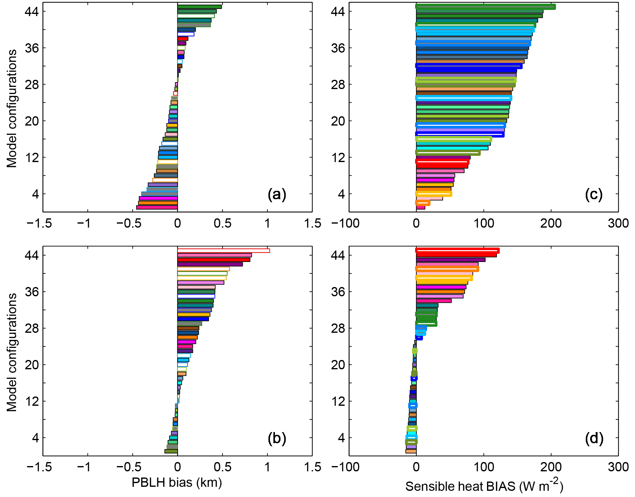
https://www.atmos-chem-phys.net/18/14813/2018/acp-18-14813-2018-f14

Figure 14Monthly averaged PBLH MBE for rawinsonde sites (a–b) and sensible heat MBE for eddy covariance sites (c–d). The two rawinsonde sites, MPX (a) and Omaha/Valley, Nebraska (OAX) (b), are close to the eddy covariance sites KUOM Turfgrass Field, Minnesota (USKUT) (c), and Mead Rainfed Maize, Nebraska (USNe3) (d), respectively. Model configurations are identified by color (see Table 1).

Download

The PBLH biases across the region show that the YSU PBL scheme tends to produce higher PBLH than the MYJ PBL scheme. This is consistent with previous studies (Hu et al., 2010; Coniglio et al., 2013; Milovac et al., 2016) that have found local PBL schemes (MYJ and MYNN) producing shallower PBLHs compared to non-local PBL schemes (YSU). As explained in Coniglio et al. (2013), the MYJ scheme produces cool and moist conditions near the ground and hence low vertical mixing, whereas the YSU scheme produces warm and dry conditions in the PBL resulting in deep mixing. Since daytime PBLH is closely linked to the surface energy balance, an additional analysis was performed using the sensible heat fluxes observed at eddy covariance stations from the AmeriFlux network (Boden et al., 2013; http://ameriflux.lbl.gov, last access: 17 January 2018). The sensible heat flux was averaged from 12:00 to 23:00 UTC, and we computed the MBE of the sensible heat flux for the eddy covariance stations close to the rawinsonde sites. The MBE was estimated at all the eddy covariance stations available over the region (not shown), and we found that the highest positive sensible heat MBEs were found on simulations that used YSU as the PBL scheme and RUC or thermal diffusion as the LSM. Figure 14 shows PBLH MBE of two rawinsonde sites (Fig. 14a, b) and the sensible heat MBE of two eddy covariance stations (Fig. 14c, d) close to each of these rawinsonde sites. We found that model configurations that use YSU as the PBL scheme in combination with RUC (Fig. 14c, d, red bars) or thermal diffusion (Fig. 14a, b, green bars) as the LSM have the highest positive bias for sensible heat flux (Fig. 14c, d), consistent with the positive biases in PBLH associated with these configurations.

We also found a spatial pattern in PBLH bias averaged over all model configurations (Fig. 9c), where the west region of the domain shows a large positive bias, with no persistent bias in the east part of the domain. This spatial gradient may be associated with the representation of warmer and drier areas in the west and cooler and moister areas in the eastern portion of the domain (Molod et al., 2015). This spatially structured PBLH bias could be associated with the choice of LSM since high biases are dominated by members using the thermal diffusion scheme (e.g., Fig. 10i, white bar with green border) in the east region of the domain and by members using RUC (e.g., Fig. 10g, red bars) in the west. Although both the RUC and thermal diffusion LSM tend to show a higher PBLH bias when the configuration includes YSU as PBL scheme, ensemble mean biases are larger in the west because RUC LSM produces higher positive bias compared to the thermal diffusion LSM. Also, we showed in Fig. 14 how these two LSMs tends to overestimate the sensible heat. These results suggest that the different LSMs could misrepresent the surface energy budget in spatially coherent ways over the region, causing spatially coherent biases in the PBLH. Cumulus parameterization also played an important role in the PBLH, as the ensemble members that did not include a cumulus parameterization produced high positive biases. This could be explained by the lack of parameterized subgrid-scale convection that could, in reality, limit PBL growth. While we were not able to find an optimal configuration across all the sites, we did find, similar to Coniglio et al. (2013) and Milovac et al. (2016), that the MYNN PBL scheme produced the smallest PBLH biases averaged over the region.

This ensemble helped us to understand and evaluate atmospheric transport errors due to physics parameterization and reanalysis, and to understand how these transport errors are propagated into simulated PBL CO₂ mole fractions. However, it is important to note several limitations of this study: (1) we explore fewer microphysics and reanalysis options (only two) compared to the number of PBL, cumulus, and LSM with three options for each; (2) this evaluation was performed over a limited period of time and location; (3) the range of parameterizations available for this sensitivity study is ad hoc and uncalibrated; and (4) the cumulus parameterizations utilized do not include parameterized transport of CO₂. We also note that some of the parameterizations (i.e., RUC LSM) were only run using the FNL reanalysis product, which may cause some underestimation of the variability as this LSM contributes significantly to the errors of all the meteorological variables. Also, as noticed in recent studies, the Grell–Freitas convection scheme produced more reliable simulations of the atmospheric dynamics (Gao et al., 2017; Gbode et al., 2018). Therefore, we recommend the use of newly developed schemes for future studies as model schemes are made available in new model versions. The impact of CP on CO₂ mole fractions requires more evaluation, because our convective scheme is not coupled with the tracers (i.e., CO₂ mole fractions); however, we can still use the convective schemes to evaluate its impact on wind fields and PBLH. Consequently, we cannot yet quantify the impact of the lack of parameterized cumulus transport of CO₂ transport on our findings. We also note that models were compared only to rawinsonde data, the only type of observation that had both the temporal and vertical resolution needed to evaluate the models within the PBL. More observations with higher temporal, spatial, and vertical resolution will be an asset for future evaluation of transport models, focusing on intensive campaigns over multiple seasons. Our meteorological results, however, are broadly consistent with past literature. The biases found in this study are a concern, since atmospheric inversions assume atmospheric transport errors are unbiased. Since this bias exists across the different meteorological variables studied here, future selection of a least biased model may need to weight the impact of each meteorological variable on CO₂ or to optimize the atmospheric transport model through a data assimilation technique. A calibrated transport ensemble may be the most efficient approach to generating an unbiased representation of atmospheric transport and associated errors.

5 Conclusions

In this study, we evaluated and quantified the atmospheric transport errors across a highly instrumented area, the Mid-Continent Intensive region of the US Midwest, for the period 18 June to 21 July 2008. Transport errors were quantified independently of flux errors and propagated into CO₂ mole fractions using a multi-physics and multi-reanalysis ensemble. Each model configuration was coupled to the same surface fluxes from CarbonTracker CT2009. We conclude that all physics parameterizations except for microphysics have a significant impact on both CO₂ mole fractions and meteorological variables. We also found that PBLH and CO₂ mole fractions have similar sensitivities to the different physics schemes. The relationship between the two variables is reinforced by the high correlations between PBLH errors and CO₂ mole fraction errors. Among the multiple configurations evaluated here, we intended to find the configuration best suited to represent the atmospheric transport over the region. However, we show no single model configuration was free from bias for every meteorological variable (PBLH, wind speed, and wind direction) and these biases vary across the domain. Some of the physics parameterization schemes tested in this study, such as the RUC LSM, YSU, and MYJ PBL schemes, showed systematic biases over the entire region, whereas the MYNN PBL scheme shows the most reasonable performance on average across the region.

The model configurations gave us additional insights into the magnitudes of the atmospheric transport errors that can be encountered over this region. However, multiple challenges remain. We showed that bias errors vary spatially across the region. If these errors persist in the transport used for a regional inversion, these biases will be propagated into the inverse fluxes. Finally, no optimal model configuration was found for the entire region. Therefore, we conclude that both random and systematic errors will remain if any one model configuration is used. An ensemble approach, possibly combined with data assimilation, could better minimize biases and characterize the spatiotemporal structures of the atmospheric transport errors for future regional inversion systems.

Code availability

The code is accessible upon request by contacting the corresponding author (lzd120@psu.edu).

Data availability

Meteorological data were obtained from the University of Wyoming's online data archive (http://weather.uwyo.edu/upperair/sounding.html, University of Wyoming, 2018) for the 14 rawinsonde stations. The tower atmospheric CO₂ concentration dataset is available online (https://daac.ornl.gov, Miles et al., 2013) from Oak Ridge National Laboratory Distributed Active Archive Center, Oak Ridge, Tennessee, USA https://doi.org/10.3334/ORNLDAAC/1202 (Miles et al., 2013). The other two towers (Park Falls – WLEF and West Branch – WBI) are part of the Earth System Research Laboratory/Global Monitoring Division (ESRL/GMD) tall tower network (Andrews et al., 2014; https://www.esrl.noaa.gov/gmd/ccgg/insitu/, Carbon Cycle and Greenhouse Gases Group, 2018). The WRF model results are accessible upon request by contacting the corresponding author (lzd120@psu.edu).

Appendix A

https://www.atmos-chem-phys.net/18/14813/2018/acp-18-14813-2018-f15

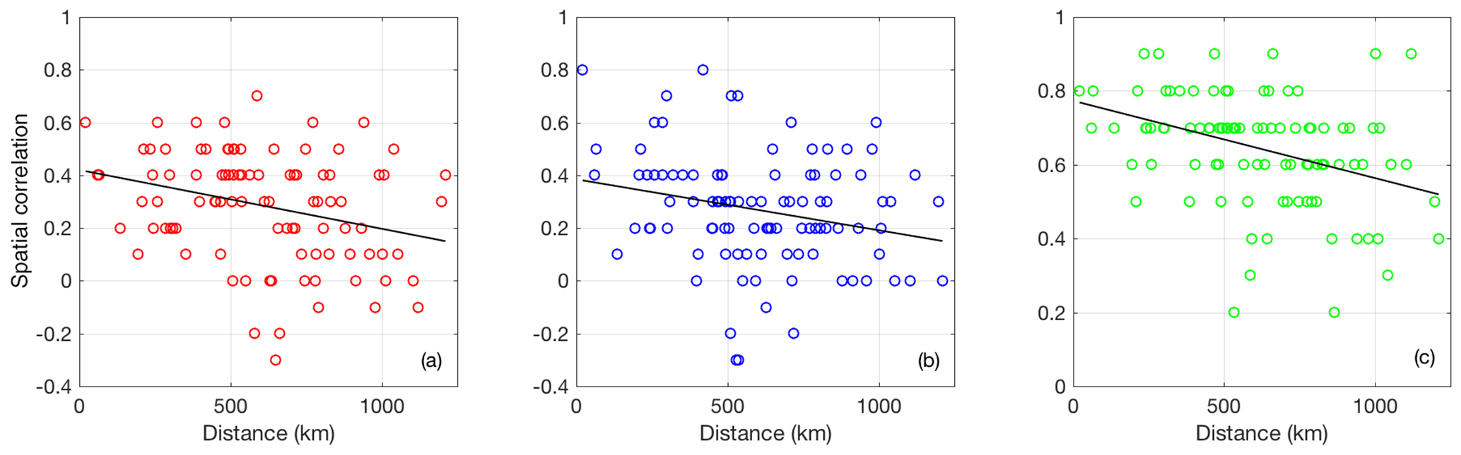
Figure A1Tower and rawinsonde sites specific spatial correlation coefficient between ensemble mean MBE of (a) wind speed, (b) wind direction, and (c) PBLH and ensemble mean MBE of DDA CO₂ mole fractions versus their distance. The abscissa shows the distance between the rawinsonde and tower sites, while the ordinate shows the spatial correlation. A line of best fit is plotted in black.

Download

Author contributions

LIDI performed the model simulations and the model–data analysis. TL provided guidance with model simulations. TL and KJD provided guidance with the model–data analysis. All authors contributed to the design of the study and the preparation the paper.

Competing interests

The authors declare that they have no conflict of interest.

Acknowledgements

This research was supported by NASA's Terrestrial Ecosystem and Carbon Cycle Program, grant NNX14AJ17G, NASA's Earth System Science Pathfinder Program Office, Earth Venture Suborbital Program, grant NNX15AG76, NASA Carbon Monitoring System, grant NNX13AP34G, and an Alfred P. Sloan Graduate Fellowship. This document benefitted from the comments of Natasha Miles, Chris E. Forest, and Andrew Carleton. Data were provided by University of Wyoming's online meteorological data archive of NOAA NWS rawinsondes, NOAA's Earth System Research Laboratory Global Monitoring Division tall tower network, the AmeriFlux network, and Penn State's contributions to the NACP Mid-Continent Intensive regional study. CarbonTracker CT2009 results were provided by NOAA ESRL, Boulder, Colorado, USA, from the website at https://www.esrl.noaa.gov/gmd/ccgg/carbontracker/ (last access: 17 January 2018).

Edited by: Mathias Palm
Reviewed by: two anonymous referees

References

Ahmadov, R., Gerbig, C., Kretschmer, R., Körner, S., Rödenbeck, C., Bousquet, P., and Ramonet, M.: Comparing high resolution WRF-VPRM simulations and two global CO₂ transport models with coastal tower measurements of CO₂, Biogeosciences, 6, 807–817, https://doi.org/10.5194/bg-6-807-2009, 2009.

Andrews, A. E., Kofler, J. D., Trudeau, M. E., Williams, J. C., Neff, D. H., Masarie, K. A., Chao, D. Y., Kitzis, D. R., Novelli, P. C., Zhao, C. L., Dlugokencky, E. J., Lang, P. M., Crotwell, M. J., Fischer, M. L., Parker, M. J., Lee, J. T., Baumann, D. D., Desai, A. R., Stanier, C. O., De Wekker, S. F. J., Wolfe, D. E., Munger, J. W., and Tans, P. P.: CO₂, CO, and CH₄ measurements from tall towers in the NOAA Earth System Research Laboratory's Global Greenhouse Gas Reference Network: instrumentation, uncertainty analysis, and recommendations for future high-accuracy greenhouse gas monitoring efforts, Atmos. Meas. Tech., 7, 647–687, https://doi.org/10.5194/amt-7-647-2014, 2014.

Baker, D. F., Law, R. M., Gurney, K. R., Rayner, P., Peylin, P., Denning, A. S., Bousquet, P., Bruhwiler, L., Chen, Y. H., Ciais, P., Fung, I. Y., Heimann, M., John, J., Maki, T., Maksyutov, S., Masarie, K., Prather, M., Pak, B., Taguchi, S., and Zhu, Z.: TransCom 3 inversion intercomparison: Impact of transport model errors on the interannual variability of regional CO₂ fluxes, 1988–2003, Global Biogeochem. Cy., 20, GB1002, https://doi.org/10.1029/2004GB002439, 2006.

Bakwin, P. S., Tans, P. P., Hurst, D. F., and Zhao, C.: Measurements of carbon dioxide on very tall towers: Results of the NOAA/CMDL program, Tellus B, 50, 401–415, https://doi.org/10.1034/j.1600-0889.1998.t01-4-00001.x, 1998.

Boden, T. A., Marland, G., and Andres, R. J.: Global, Regional, and National Fossil-Fuel CO₂ Emissions, Carbon Dioxide Inf. Anal. Cent. Oak Ridge Natl. Lab. USA Oak Ridge TN Dep. Energy, U.S. Department of Energy, Oak Ridge, Tennessee, https://doi.org/10.3334/CDIAC/00001, 2009.

Boden, T. A., Krassovski, M., and Yang, B.: The AmeriFlux data activity and data system: an evolving collection of data management techniques, tools, products and services, Geosci. Instrum. Meth., 2, 165–176, 2013.

Bousquet, P., Peylin, P., Ciais, P., Le Quere, C., Friedlingstein, P., and Tans, P. P.: Regional changes in carbon dioxide fluxes of land and oceans since 1980, Science, 290, 1342–1346, 2000

Brooks, B.-G. J., Desai, A. R., Stephens, B. B., Bowling, D. R., Burns, S. P., Watt, A. S., Heck, S. L., and Sweeney, C.: Assessing filtering of mountaintop CO₂ mole fractions for application to inverse models of biosphere-atmosphere carbon exchange, Atmos. Chem. Phys., 12, 2099–2115, https://doi.org/10.5194/acp-12-2099-2012, 2012.

Carbon Cycle and Greenhouse Gases Group: Global Greenhouse Gas Reference Network, available at: https://www.esrl.noaa.gov/gmd/ccgg/insitu/, last access: 20 July 2018.

Chen, F. and Dudhia, J.: Coupling an Advanced Land Surface–Hydrology Model with the Penn State–NCAR MM5 Modeling System. Part I: Model Implementation and Sensitivity, Mon. Weather Rev., 129, 569–585, 2001.

Cheng, W. Y. Y. and Steenburgh, W. J.: Evaluation of Surface Sensible Weather Forecasts by the WRF and the Eta Models over the Western United States, Weather Forecast., 20, 812–821, https://doi.org/10.1175/WAF885.1, 2005.

Chevallier, F., Ciais, P., Conway, T. J., Aalto, T., Anderson, B. E., Bousquet, P., Brunke, E. G., Ciattaglia, L., Esaki, Y., Fröhlich, M., Gomez, A., Gomez-Pelaez, A. J., Haszpra, L., Krummel, P. B., Langenfelds, R. L., Leuenberger, M., MacHida, T., Maignan, F., Matsueda, H., Morguí, J. A., Mukai, H., Nakazawa, T., Peylin, P., Ramonet, M., Rivier, L., Sawa, Y., Schmidt, M., Steele, L. P., Vay, S. A., Vermeulen, A. T., Wofsy, S., and Worthy, D.: CO₂ surface fluxes at grid point scale estimated from a global 21 year reanalysis of atmospheric measurements, J. Geophys. Res.-Atmos., 115, D21307, https://doi.org/10.1029/2010JD013887, 2010.

Ciais, P., Tans, P. P., Trolier, M., White, J. W. C., and Francey, R. J.: A Large Northern Hemisphere Terrestrial CO₂ Sink Indicated by the 13C/12C Ratio of Atmospheric CO₂, Science, 269, 1098–1102, https://doi.org/10.1126/science.269.5227.1098, 1995.

Coniglio, M. C., Correia, J., Marsh, P. T., and Kong, F.: Verification of Convection-Allowing WRF Model Forecasts of the Planetary Boundary Layer Using Sounding Observations, Weather Forecast., 28, 842–862, https://doi.org/10.1175/WAF-D-12-00103.1, 2013.

Davis, K. J., Bakwin, P. S., Yi, C., Berger, B. W., Zhao, C., Teclaw, R. M., and Isebrands, J. G.: The annual cycles of CO₂ and H2O exchange over a northern mixed forest as observed from a very tall tower, Glob. Change Biol., 9, 1278–1293, https://doi.org/10.1046/j.1365-2486.2003.00672.x, 2003.

Deng, A., Lauvaux, T., Davis, K. J., Gaudet, B. J., Miles, N., Richardson, S. J., Wu, K., Sarmiento, D. P., Hardesty, R. M., Bonin, T. A., Brewer, W. A., and Gurney, K. R.: Toward reduced transport errors in a high resolution urban CO₂ inversion system, Elem. Sci. Anth., 5, 20, https://doi.org/10.1525/elementa.133,2017.

Denning, A. S., Fung, I. Y., and Randall, D.: Latitudinal gradient of atmospheric CO₂ due to seasonal exchange with land biota, Nature, 376, 240–243, https://doi.org/10.1038/376240a0, 1995.

Díaz Isaac, L. I., Lauvaux, T., Davis, K. J., Miles, N. L., Richardson, S. J., Jacobson, A. R., and Andrews, A. E.: Model-data comparison of MCI field campaign atmospheric CO 2 mole fractions, J. Geophys. Res.-Atmos., 119, 10536–10551, https://doi.org/10.1002/2014JD021593, 2014.

Dudhia, J.: A multi-layer soil temperature model for MM5, Preprints, The sixth PSU/NCAR Mesoscale Model Users Work- shop, 22–24 July 1996, Boulder, Colorado, 49–50, 1996.

Enting, I. G.: Inverse problems in atmospheric constituent studies: III. Estimating errors in surface sources, Inverse Probl., 9, 649–665, https://doi.org/10.1088/0266-5611/9/6/004, 1993.

Feng, S., Lauvaux, T., Newman, S., Rao, P., Ahmadov, R., Deng, A., Díaz-Isaac, L. I., Duren, R. M., Fischer, M. L., Gerbig, C., Gurney, K. R., Huang, J., Jeong, S., Li, Z., Miller, C. E., O'Keeffe, D., Patarasuk, R., Sander, S. P., Song, Y., Wong, K. W., and Yung, Y. L.: Los Angeles megacity: a high-resolution land-atmosphere modelling system for urban CO₂ emissions, Atmos. Chem. Phys., 16, 9019–9045, https://doi.org/10.5194/acp-16-9019-2016, 2016.

Fovell, R. G. and Cao, Y.: Wind and gust forecasting in complex terrain. Preprints, Annual WRF Users' Workshop, Boulder, CO, NCAR, 2014.

Gao, Y., Leung, L. R., Zhao, C., and Hagos, S.: Sensitivity ofUS summerprecipitation to model resolution and convective parameterizations across gray zone resolutions. J. Geophys. Res.-Atmos., 122, 2714–2733, https://doi.org/10.1002/2016JD025896, 2017.

Gbode, I. E., Dudhia, J., Ogunjobi, K. O., and Ojayi, V. O.: Sensitivity of different physics schemes in the WRF model during a West African monsoon regim, Theor. Appl. Climatol., 1–19, 1–19, https://doi.org/10.1007/s00704-018-2538-x, 2018.

Gerbig, C., Körner, S., and Lin, J. C.: Vertical mixing in atmospheric tracer transport models: error characterization and propagation, Atmos. Chem. Phys., 8, 591–602, https://doi.org/10.5194/acp-8-591-2008, 2008.

Giglio, L., Csiszar, I., and Justice, C. O.: Global distribution and seasonality of active fires as observed with the Terra and Aqua Moderate Resolution Imaging Spectroradiometer (MODIS) sensors, J. Geophys. Res.-Biogeosci., 111, G02016, https://doi.org/10.1029/2005JG000142, 2006.

Gloor, M., Gruber, N., Sarmiento, J., Sabine, C. L., Feely, R. A., and Rödenbeck, C.: A first estimate of present and preindustrial air-sea CO₂ flux patterns based on ocean interior carbon measurements and models, Geophys. Res. Lett., 30, 1010, https://doi.org/10.1029/2002GL015594, 2003.

Grell, G. and Devenyi, D.: A generalized approach to pa- rameterizing convection combining ensemble and data assimilation techniques, Geophys. Res. Lett., 29, https://doi.org/10.1029/2002GL015311, 2002.

Grell, G. A.: Prognostic evaluation of assumptions used by cumulus parameterizations within a generalized framework, Mon. Weather Rev., 121, 764–787, 1993.

Gruber, N., Sarmiento, J. L., and Stocker, T. F.: An Improved Method for Detecting Anthropogenic CO₂ in the Oceans, Global Biogeochem. Cy., 10, 809–837, https://doi.org/10.1029/96GB01608, 1996.

Gurney, K. R., Law, R. M., Denning, a S., Rayner, P. J., Baker, D., Bousquet, P., Bruhwiler, L., Chen, Y.-H., Ciais, P., Fan, S., Fung, I. Y., Gloor, M., Heimann, M., Higuchi, K., John, J., Maki, T., Maksyutov, S., Masarie, K., Peylin, P., Prather, M., Pak, B. C., Randerson, J., Sarmiento, J., Taguchi, S., Takahashi, T., and Yuen, C.-W.: Towards robust regional estimates of CO₂ sources and sinks using atmospheric transport models, Nature, 415, 626–630, https://doi.org/10.1038/415626a, 2002.

Hong, S.-Y., Dudhia, J., and Chen, S.-H.: A Revised Approach to Ice Microphysical Processes for the Bulk Parameterization of Clouds and Precipitation, Mon. Weather Rev., 132, 103–120, 2004.

Hong, S.-Y., Noh, Y., and Dudhia, J.: A new vertical diffusion package with an explicit treatment of entrainment processes., Mon. Weather Rev., 134, 2318–2341, https://doi.org/10.1175/MWR3199.1, 2006.

Hu, X. M., Nielsen-Gammon, J. W., and Zhang, F.: Evaluation of three planetary boundary layer schemes in the WRF model, J. Appl. Meteorol. Clim., 49, 1831–1844, https://doi.org/10.1175/2010JAMC2432.1, 2010.

Huntzinger, D. N., Post, W. M., Wei, Y., Michalak, A. M., West, T. O., Jacobson, A. R., Baker, I. T., Chen, J. M., Davis, K. J., Hayes, D. J., Hoffman, F. M., Jain, A. K., Liu, S., McGuire, A. D., Neilson, R. P., Potter, C., Poulter, B., Price, D., Raczka, B. M., Tian, H. Q., Thornton, P., Tomelleri, E., Viovy, N., Xiao, J., Yuan, W., Zeng, N., Zhao, M., and Cook, R.: North American Carbon Program (NACP) regional interim synthesis: Terrestrial biospheric model intercomparison, Ecol. Model., 232, 144–157, https://doi.org/10.1016/J.Ecolmodel.2012.02.004, 2012.

IPCC: Climate Change 2013, The Physical Science Basis, Contri- bution of Working Group I to the Fifth Assessment Report of the Intergovernmental Panel on Climate Change, edited by: Stocker, T. F., Qin, D., Plattner, G.-K., Tignor, M., Allen, S. K., Boschung, J., Nauels, A., Xia, Y., Bex, V., and Midgley, P. M., Cambridge University Press, Tech. rep., 2013.

Jacobson, A. R., Fletcher, S. E. M., Gruber, N., Sarmiento, J. L., and Gloor, M.: A joint atmosphere-ocean inversion for surface fluxes of carbon dioxide: 1. Methods and global-scale fluxes, Global Biogeochem. Cy., 21, GB1019, https://doi.org/10.1029/2005GB002556, 2007.

Janjic, Z.: Nonsingular implementation of the Mellor-Yamada level 2.5 scheme in the NCEP Meso model, National Centers for Environmental Prediction, USA, Office Note No. 437, 2002.

Jimenez, P. A. and Dudhia, J.: Improving the representation of re- solved and unresolved topographic effects on surface wind in the WRF Model, J. Appl. Meteorol. Clim., 51, 300–316, 2012.

Kain, J. S.: The Kain–Fritsch Convective Parameterization: An Update, J. Appl. Meteorol., 43, 170–181, 2004.

Kretschmer, R., Gerbig, C., Karstens, U., and Koch, F.-T.: Error characterization of CO₂ vertical mixing in the atmospheric transport model WRF-VPRM, Atmos. Chem. Phys., 12, 2441–2458, https://doi.org/10.5194/acp-12-2441-2012, 2012.

Kretschmer, R., Gerbig, C., Karstens, U., Biavati, G., Vermeulen, A., Vogel, F., Hammer, S., and Totsche, K. U.: Impact of optimized mixing heights on simulated regional atmospheric transport of CO₂, Atmos. Chem. Phys., 14, 7149–7172, https://doi.org/10.5194/acp-14-7149-2014, 2014.

Krol, M., Houweling, S., Bregman, B., van den Broek, M., Segers, A., van Velthoven, P., Peters, W., Dentener, F., and Bergamaschi, P.: The two-way nested global chemistry-transport zoom model TM5: algorithm and applications, Atmos. Chem. Phys., 5, 417–432, https://doi.org/10.5194/acp-5-417-2005, 2005.

Lauvaux, T. and Davis, K. J.: Planetary boundary layer errors in mesoscale inversions of column-integrated CO₂ measurements, J. Geophys. Res.-Atmos., 119, 490–508, https://doi.org/10.1002/2013JD020175, 2014.

Lauvaux, T., Schuh, A. E., Uliasz, M., Richardson, S., Miles, N., Andrews, A. E., Sweeney, C., Diaz, L. I., Martins, D., Shepson, P. B., and Davis, K. J.: Constraining the CO₂ budget of the corn belt: exploring uncertainties from the assumptions in a mesoscale inverse system, Atmos. Chem. Phys., 12, 337–354, https://doi.org/10.5194/acp-12-337-2012, 2012.

Law, R. M., Chen, Y. H., and Gurney, K. R.: TransCom-3 CO₂ inversion intercomparison: 2. Sensitivity of annual mean results to data choices, Tellus B, 55, 580–595, 2003.

Law, R. M., Peters, W., Rödenbeck, C., Aulagnier, C., Baker, I., Bergmann, D. J., Bousquet, P., Brandt, J., Bruhwiler, L., Cameron-Smith, P. J., Christensen, J. H., Delage, F., Denning, A. S., Fan, S., Geels, C., Houweling, S., Imasu, R., Karstens, U., Kawa, S. R., Kleist, J., Krol, M. C., Lin, S. J., Lokupitiya, R., Maki, T., Maksyutov, S., Niwa, Y., Onishi, R., Parazoo, N., Patra, P. K., Pieterse, G., Rivier, L., Satoh, M., Serrar, S., Taguchi, S., Takigawa, M., Vautard, R., Vermeulen, A. T., and Zhu, Z.: TransCom model simulations of hourly atmospheric CO₂: Experimental overview and diurnal cycle results for 2002, Global Biogeochem. Cy., 22, GB3009, https://doi.org/10.1029/2007GB003050, 2008.

Le Quéré, C., Moriarty, R., Andrew, R. M., Canadell, J. G., Sitch, S., Korsbakken, J. I., Friedlingstein, P., Peters, G. P., Andres, R. J., Boden, T. A., Houghton, R. A., House, J. I., Keeling, R. F., Tans, P., Arneth, A., Bakker, D. C. E., Barbero, L., Bopp, L., Chang, J., Chevallier, F., Chini, L. P., Ciais, P., Fader, M., Feely, R. A., Gkritzalis, T., Harris, I., Hauck, J., Ilyina, T., Jain, A. K., Kato, E., Kitidis, V., Klein Goldewijk, K., Koven, C., Landschützer, P., Lauvset, S. K., Lefèvre, N., Lenton, A., Lima, I. D., Metzl, N., Millero, F., Munro, D. R., Murata, A., Nabel, J. E. M. S., Nakaoka, S., Nojiri, Y., O'Brien, K., Olsen, A., Ono, T., Pérez, F. F., Pfeil, B., Pierrot, D., Poulter, B., Rehder, G., Rödenbeck, C., Saito, S., Schuster, U., Schwinger, J., Séférian, R., Steinhoff, T., Stocker, B. D., Sutton, A. J., Takahashi, T., Tilbrook, B., van der Laan-Luijkx, I. T., van der Werf, G. R., van Heuven, S., Vandemark, D., Viovy, N., Wiltshire, A., Zaehle, S., and Zeng, N.: Global Carbon Budget 2015, Earth Syst. Sci. Data, 7, 349–396, https://doi.org/10.5194/essd-7-349-2015, 2015.

Mesinger, F., DiMego, G., Kalnay, E., Mitchell, K., Shafran, P. C., Ebisuzaki, W., Jović, D., Woollen, J., Rogers, E., Berbery, E. H., Ek, M. B., Fan, Y., Grumbine, R., Higgins, W., Li, H., Lin, Y., Manikin, G., Parrish, D., and Shi, W.: North American regional reanalysis, B. Am. Meteorol. Soc., 87, 343–360, https://doi.org/10.1175/BAMS-87-3-343, 2006.

Miles, N. L., Richardson, S. J., Davis, K. J., Lauvaux, T., Andrews, A. E., West, T. O., Bandaru, V., and Crosson, E. R.: Large amplitude spatial and temporal gradients in atmospheric boundary layer CO₂ mole fractions detected with a tower-based network in the U.S. upper Midwest, J. Geophys. Res.-Biogeosci., 117, 01019, https://doi.org/10.1029/2011JG001781, 2012.

Miles, N. L., Richardson, S. J., Davis, K. J., Andrews, A. E., Griffis,T. J., Bandaru, V., and Hosman, K. P.: NACP MCI: Tower Atmospheric CO₂ Concentrations, Upper Midwest Region, USA, 2007–2009, Oak Ridge National Laboratory Distributed Active Archive Center, Oak Ridge, Tennessee, USA, https://doi.org/10.3334/ORNLDAAC/1202, 2013.

Milovac, J., Warrach-Sagi, K., Behrendt, A., Späth, F., Ingwersen, J., and Wulfmeyer, V.: Investigation of PBL schemes combining the WRF model simulations with scanning water vapour differential absorption lidar measurements, J. Geophys. Res.-Atmos, 121, 624–649, https://doi.org/10.1002/2015JD023927, 2016.

Molod, A., Salmun, H., and Dempsey, M.: Estimating planetary boundary layer heights from NOAA Profiler Network wind profiler data, J. Atmos. Ocean. Tech., 32, 1545–1561, https://doi.org/10.1175/JTECH-D-14-00155.1, 2015.

Nakanishi, M. and Niino, H.: An improved Mellor-Yamada Level-3 model with condensation physics: Its design and verification, Bound.-Lay. Meteorol., 112, 1–31, https://doi.org/10.1023/B:BOUN.0000020164.04146.98, 2004.

Ogle, S., Davis, K. J., Andrews, A. E., Gurney, K. R., West, T. O., Cooke, R. B., Parkin, T., Morissette, J., Verma, S., and Wofsy, S.: Science plan: Mid-Continent Intensive Campaign of the North American Carbon Program, NACP, Greenbel, MD, 2006.

Olivier, J. G. J., Berdowski, J. J. M., Peters, J. A. H. W., Bakker, J., Visschedijk en, A. J. H., and Bloos, J.-P. J.: Applications of EDGAR. Including a description of EDGAR 3.0: reference database with trend data for 1970–1995, RIVM, Bilthoven, RIVM report no. 773301 001/ NOP report no. 410200 051, 2001.

Olsen, S. and Randerson, J: Difference between surface and column atmospheric CO₂ and implications for carbon cycle research, J. Geophys. Res., 109, D02301, https://doi.org/10.1029/2003JD003968,2004.

Pan, Y., Birdsey, R. A., Fang, J., Houghton, R., Kauppi, P. E., Kurz, W. A., Phillips, O. L., Shvidenko, A., Lewis, S. L., Canadell, J. G., Ciais, P., Jackson, R. B., Pacala, S. W., McGuire, A. D., Piao, S., Rautiainen, A., Sitch, S., and Hayes, D.: A large and persistent carbon sink in the world's forests, Science, 333, 988–993, https://doi.org/10.1126/science.1201609, 2011.

Patra, P. K., Law, R. M., Peters, W., Rödenbeck, C., Takigawa, M., Aulagnier, C., Baker, I., Bergmann, D. J., Bousquet, P., Brandt, J., Bruhwiler, L., Cameron-Smith, P. J., Christensen, J. H., Delage, F., Denning, A. S., Fan, S., Geels, C., Houweling, S., Imasu, R., Karstens, U., Kawa, S. R., Kleist, J., Krol, M. C., Lin, S. J., Lokupitiya, R., Maki, T., Maksyutov, S., Niwa, Y., Onishi, R., Parazoo, N., Pieterse, G., Rivier, L., Satoh, M., Serrar, S., Taguchi, S., Vautard, R., Vermeulen, A. T., and Zhu, Z.: TransCom model simulations of hourly atmospheric CO₂: Analysis of synoptic-scale variations for the period 2002–2003, Global Biogeochem. Cy., 22, GB4013, https://doi.org/10.1029/2007GB003081, 2008.

Pei, L., Moore, N., Zhong, S., Luo, L., Hyndman, D. W., Heilman, W. E., and Gao, Z.: WRF model sensitivity to land surface model and cumulus parameterization under short-term climate extremes over the Southern great plains of the United States, J. Climate, 27, 7703–7724, https://doi.org/10.1175/JCLI-D-14-00015.1, 2014.

Peters, W., Jacobson, A. R., Sweeney, C., Andrews, A. E., Conway, T. J., Masarie, K., Miller, J. B., Bruhwiler, L. M. P., Pétron, G., Hirsch, A. I., Worthy, D. E. J., van der Werf, G. R., Randerson, J. T., Wennberg, P. O., Krol, M. C., and Tans, P. P.: An atmospheric perspective on North American carbon dioxide exchange: CarbonTracker, P. Natl. Acad. Sci. USA, 104, 18925–18930, https://doi.org/10.1073/pnas.0708986104, 2007.

Peylin, P., Law, R. M., Gurney, K. R., Chevallier, F., Jacobson, A. R., Maki, T., Niwa, Y., Patra, P. K., Peters, W., Rayner, P. J., Rödenbeck, C., van der Laan-Luijkx, I. T., and Zhang, X.: Global atmospheric carbon budget: results from an ensemble of atmospheric CO₂ inversions, Biogeosciences, 10, 6699–6720, https://doi.org/10.5194/bg-10-6699-2013, 2013.

Pickett-Heaps, C. A., Rayner, P. J., Law, R. M., Ciais, P., Patra, P. K., Bousquet, P., Peylin, P., Maksyutov, S., Marshall, J., Rödenbeck, C., Langenfelds, R. L., Steele, L. P., Francey, R. J., Tans, P., and Sweeney, C.: Atmospheric CO₂ inversion validation using vertical profile measurements: Analysis of four independent inversion models, J. Geophys. Res.-Atmos., 116, 3773–3779, https://doi.org/10.1029/2010JD014887, 2011.

Richardson, S. J., Miles, N. L., Davis, K. J., Crosson, E. R., Rella, C. W., and Andrews, A. E.: Field testing of cavity ring-down spectroscopy analyzers measuring carbon dioxide and water vapor, J. Atmos. Ocean. Tech., 29, 397–406, https://doi.org/10.1175/JTECH-D-11-00063.1, 2012.

Román-Cascón, C., Yagüe, C., Sastre, M., Maqueda, G., Salamanca, F., and Viana, S.: Observations and WRF simulations of fog events at the Spanish Northern Plateau, Adv. Sci. Res., 8, 11–18, https://doi.org/10.5194/asr-8-11-2012, 2012.

Roux, G., Liu, Y., Monache, L. D., Sheu, R.-S., and Warner, T. T.: Verification of high resolution WRF-RTFDDA surface forecasts over mountains and plains. Preprints, WRF Users' Workshop, Boulder, CO, NCAR, 2009.

Santos-Alamillos, F., Pozo-Vaìzquez D., Ruiz-Arias, J. A., Lara-Fanego, V., and Tovar-Pescador, J.: Analysis of WRF model wind estimate sensitivity to physics parameterization choice and terrain representation in Andalusia (Southern Spain), J. Appl. Meteorol. Clim., 52, 1592–1609, https://doi.org/10.1175/JAMC-D-12-0204.1,2013.

Sarmiento, J. L., Gloor, M., Gruber, N., Beaulieu, C., Jacobson, A. R., Mikaloff Fletcher, S. E., Pacala, S., and Rodgers, K.: Trends and regional distributions of land and ocean carbon sinks, Biogeosciences, 7, 2351–2367, https://doi.org/10.5194/bg-7-2351-2010, 2010.

Sarrat, C., Noilhan, J., Lacarrère, P., Donier, S., Dolman, H., Gerbig, C., Ciais, P., and Butet, A.: Atmospheric CO₂ modeling at the regional scale: Application to the CarboEurope Regional Experiment, J. Geophys. Res., 112, D12105, https://doi.org/10.1029/2006JD008107, 2007.

Skamarock, W. C., Klemp, J. B., Dudhia, J., Gill, D. O., Barker, D. M., Duda, M., Huang, X. Y., Wang, W., and Powers, J. G.: A description of the advanced research WRF version 3, NCAR, Tech. Note, Mesoscale and Microscale Meteorology Division, National Center for Atmospheric Research, Boulder, Colorado, USA, 2008.

Smirnova, T. G., Brown, J. M., Benjamin, S. G., and Kim, D.: Parameterization of cold-season processes in the MAPS land-surface scheme, J. Geophys. Res., 105, 4077, https://doi.org/10.1029/1999JD901047, 2000.

Soriano, C., Jorba, O., and Baldasano, J. M.: One-way nesting versus two-way nesting: Does it really make a difference? Air Pollution Modelling and Its Application XV, edited by: Borrego, C. and Schayes, G., Kluwer Academic, 177–185, 2002.

Stephens, B. B., Gurney, K. R., Tans, P. P., Sweeney, C., Peters, W., Bruhwiler, L., Ciais, P., Ramonet, M., Bousquet, P., Nakazawa, T., Aoki, S., Machida, T., Inoue, G., Vinnichenko, N., Lloyd, J., Jordan, A., Heimann, M., Shibistova, O., Langenfelds, R. L., Steele, L. P., Francey, R. J., and Denning, A. S.: Weak northern and strong tropical land carbon uptake from vertical profiles of atmospheric CO₂, Science, 316, 1732–1735, https://doi.org/10.1126/science.1137004, 2007.

Stull, R. B.: An Introduction to Boundary Layer Meteorology, Kluwer Academic, 666 pp., 1988.

Tans, P. P., Fung, I. Y., and Takahashi, T.: Observational constraints on the Global Atmospheric CO₂ budget, Science, 247, 1431–1438, https://doi.org/10.1126/science.247.4949.1431, 1990.

Tarantola, A.: Inverse problem theory and methods for model parameter estimation, Society for Industrial and Applied Mathematics, Philadelphia, PA, 2005.

Taylor, K. E.: Summarizing multiple aspects of model performance in a single diagram, J. Geophys. Res., 106, 7183–7192, 2001.

Thompson, G., Rasmussen, R. M., and Manning, K.: Explicit Forecasts of Winter Precipitation Using an Improved Bulk Microphysics Scheme. Part I: Description and Sensitivity Analysis, Mon. Weather Rev., 132, 519–542, 2004.

University of Wyoming: Upper Air Observations, availabel at: http://weather.uwyo.edu/upperair/sounding.html, last access date: 20 July 2018.

van der Werf, G. R., Randerson, J. T., Giglio, L., Collatz, G. J., Kasibhatla, P. S., and Arellano Jr., A. F.: Interannual variability in global biomass burning emissions from 1997 to 2004, Atmos. Chem. Phys., 6, 3423–3441, https://doi.org/10.5194/acp-6-3423-2006, 2006.

Wang, W., Davis, K. J., Yi, C., Patton, E. G., Butler, M. P., Ricciuto, D. M., and Bakwin, P. S.: A note on the top-down and bottom-up gradient functions over a forested site, Bound. Lay. Meteorol., 124, 305–314, 2007.

Wilks, D. S.: Statistical Methods in the Atmospheric Sciences, 3rd ed. Oxford, Waltham, MA: Academic Press, 2011.

Yerramilli, A., Challa, V. S., Dodla, V. B. R., Dasari, H. P., Young, J. H., Patrick, C., Baham, J. M., Hughes, R. L., Hardy, M. G., and Swanier, S. J.: Simulation of Surface Ozone Pollution in the Central Gulf Coast Region Using WRF/Chem Model: Sensitivity to PBL and Land Surface Physics, Adv. Meteorol., 2010, 1–24, https://doi.org/10.1155/2010/319138, 2010.

Yi, C., Davis, K. J., Bakwin, P. S., Denning, A. S., Zhang, N., Desai, A., Lin, J. C., and Gerbig, C.: Observed covariance between ecosystem carbon exchange and atmospheric boundary layer dynamics at a site in northern Wisconsin, J. Geophys. Res.-Atmos., 109, D08302, https://doi.org/10.1029/2003JD004164, 2004.

Yver, C. E., Graven, H. D., Lucas, D. D., Cameron-Smith, P. J., Keeling, R. F., and Weiss, R. F.: Evaluating transport in the WRF model along the California coast, Atmos. Chem. Phys., 13, 1837–1852, https://doi.org/10.5194/acp-13-1837-2013, 2013.

Zhang, Y., Dubey, M. K., Olsen, S. C., Zheng, J., and Zhang, R.: Comparisons of WRF/Chem simulations in Mexico City with ground-based RAMA measurements during the 2006-MILAGRO, Atmos. Chem. Phys., 9, 3777–3798, https://doi.org/10.5194/acp-9-3777-2009, 2009.

CarbonTracker CT2009, https://www.esrl.noaa.gov/gmd/ccgg/carbontracker/ (last access: 17 January 2018)

Articles

Short summary

Atmospheric inversions rely on the accurate representation of the atmospheric dynamics in order to produce reliable surface fluxes. In this work, we evaluate the sensitivity of a state-of-the-art mesoscale atmospheric model to the different physics parameterizations and forcing. We conclude that no model configuration is optimal across an entire region. Therefore, we recommend an ensemble approach or the assimilation of meteorological observations in future inversion studies.

Impact of physical parameterizations and initial conditions on simulated atmospheric transport and CO2 mole fractions in the US Midwest

2.1 Region

2.2 Atmospheric model setup

2.3 Ensemble configuration

2.4 Physics parameterization schemes

2.4.1 Land surface models (LSMs)

2.4.2 Planetary boundary layer (PBL) schemes

2.4.3 Cumulus parameterizations

2.4.4 Microphysics parameterizations

2.5 Meteorological initial and boundary conditions

2.6 CO2 surface fluxes

2.7 Dataset

2.8 Data selection

2.9 Evaluation methodology or analyses of the models

2.9.1 Analyses of physics parameterization and reanalyses impact

2.9.2 Analyses of model–data residuals

3.1 Impact of physics parameterizations on atmospheric CO2 mole fractions

3.2 Meteorological day-to-day variability

3.3 Characterization of transport errors

3.3.1 Root mean square error (RMSE)

3.3.2 Mean bias error (MBE)

3.4 Sensitivity of CO2 mole fractions to model configuration

Impact of physical parameterizations and initial conditions on simulated atmospheric transport and CO₂ mole fractions in the US Midwest

2.6 CO₂ surface fluxes

3.1 Impact of physics parameterizations on atmospheric CO₂ mole fractions

3.4 Sensitivity of CO₂ mole fractions to model configuration