the Creative Commons Attribution 4.0 License.
the Creative Commons Attribution 4.0 License.
 | 12 Oct 2018
Comparison of mean age of air in five reanalyses using the BASCOE transport model
Simon Chabrillat
Corinne Vigouroux
Yves Christophe
Andreas Engel
Quentin Errera
Daniele Minganti
Beatriz M. Monge-Sanz
Arjo Segers
Emmanuel Mahieu
We present a consistent intercomparison of the mean age of air (AoA) according to five modern reanalyses: the European Centre for Medium-Range Weather Forecasts Interim Reanalysis (ERA-Interim), the Japanese Meteorological Agency's Japanese 55-year Reanalysis (JRA-55), the National Centers for Environmental Prediction Climate Forecast System Reanalysis (CFSR) and the National Aeronautics and Space Administration's Modern Era Retrospective analysis for Research and Applications version 1 (MERRA) and version 2 (MERRA-2). The modeling tool is a kinematic transport model driven only by the surface pressure and wind fields. It is validated for ERA-I through a comparison with the AoA computed by another transport model.
The five reanalyses deliver AoA which differs in the worst case by 1 year in the tropical lower stratosphere and more than 2 years in the upper stratosphere. At all latitudes and altitudes, MERRA-2 and MERRA provide the oldest values (∼5–6 years in midstratosphere at midlatitudes), while JRA-55 and CFSR provide the youngest values (∼4 years) and ERA-I delivers intermediate results. The spread of AoA at 50 hPa is as large as the spread obtained in a comparison of chemistry–climate models. The differences between tropical and midlatitude AoA are in better agreement except for MERRA-2. Compared with in situ observations, they indicate that the upwelling is too fast in the tropical lower stratosphere. The spread between the five simulations in the northern midlatitudes is as large as the observational uncertainties in a multidecadal time series of balloon observations, i.e., approximately 2 years. No global impact of the Pinatubo eruption can be found in our simulations of AoA, contrary to a recent study which used a diabatic transport model driven by ERA-I and JRA-55 winds and heating rates.
The time variations are also analyzed through multiple linear regression analyses taking into account the seasonal cycles, the quasi-biennial oscillation and the linear trends over four time periods. The amplitudes of AoA seasonal variations in the lower stratosphere are significantly larger when using MERRA and MERRA-2 than with the other reanalyses. The linear trends of AoA using ERA-I confirm those found by earlier model studies, especially for the period 2002–2012, where the dipole structure of the latitude–height distribution (positive in the northern midstratosphere and negative in the southern midstratosphere) also matches trends derived from satellite observations of SF6. Yet the linear trends vary substantially depending on the considered period. Over 2002–2015, the ERA-I results still show a dipole structure with positive trends in the Northern Hemisphere reaching up to 0.3 yr dec−1. No reanalysis other than ERA-I finds any dipole structure of AoA trends. The signs of the trends depend strongly on the input reanalysis and on the considered period, with values above 10 hPa varying between approximately −0.4 and 0.4 yr dec−1. Using ERA-I and CFSR, the 2002–2015 trends are negative above 10 hPa, but using the three other reanalyses these trends are positive. Over the whole period (1989–2015) each reanalysis delivers opposite trends; i.e., AoA is mostly increasing with CFSR and ERA-I but mostly decreasing with MERRA, JRA-55 and MERRA-2.
In view of this large disagreement, we urge great caution for studies aiming to assess AoA trends derived only from reanalysis winds. We briefly discuss some possible causes for the dependency of AoA on the input reanalysis and highlight the need for complementary intercomparisons using diabatic transport models.
- Article
(3320 KB) -
Supplement
(17557 KB) - BibTeX
- EndNote


The mean age of air (hereafter AoA) is an evaluation of the time necessary for variations of long-lived (e.g., greenhouse or ozone-depleting) species to propagate from the troposphere to various regions in the stratosphere. This classical diagnostic provides insights on the strength and structure of the Brewer–Dobson circulation (BDC), the polar vortex and irreversible mixing in the midlatitudes (Waugh and Hall, 2002). Due to increased greenhouse gas forcing, chemistry–climate model (CCM) simulations of the 1990–2090 period predict an acceleration of the BDC and a decrease of AoA at all latitudes in the lower part of the stratosphere (Austin and Li, 2006; Butchart, 2014). The observational detection of trends in the BDC strength turns out to be quite difficult. They can be indirectly derived from multidecadal records of stratospheric temperatures but these derivations are indirect and do not yet allow a clear confirmation of the acceleration predicted by CCM, mainly due to an insufficiently constrained accuracy of the temperature observations (Fu et al., 2015; Ossó et al., 2015).
Observation-based AoA is derived from concentration measurements of very long-lived tracers which increase (nearly) monotonically at the surface, such as CO2 or SF6. Multidecadal datasets were compiled from balloon soundings or aircraft flights (Andrews et al., 2001; Ray et al., 2014). The corresponding time series are precise but sparse in time and space, leading to large sampling uncertainties. Global coverage time series have been derived from satellite observations, but the precision is lower. The SF6 retrievals from the Michelson Interferometer for Passive Atmospheric Sounding (MIPAS) satellite instrument delivered a continuously updated dataset with global coverage for the period 2002–2012, leading to breakthrough studies about observed AoA and its time variations during this comparatively short period (Haenel et al., 2015; Stiller et al., 2008). The magnitude, distribution and detectability of the AoA trends observed over the past years and decades are currently a topic of intense research (Engel et al., 2009, 2017; Mahieu et al., 2014; Stiller et al., 2012).
Reanalysis systems combine a global weather forecast model, observations and an assimilation scheme to provide the best estimates (analyses) of past atmospheric states including surface pressure, temperature and wind over a long (usually multidecadal) period. While they are derived from assimilation systems used operationally to deliver weather forecasts, they aim to achieve more consistent variations over long timescales, e.g., avoiding spurious discontinuities and trends (Bengtsson and Shukla, 1988; Trenberth and Olson, 1988). Hence, the same model version and assimilation scheme are used for the whole period and special care is given to the time-varying biases between the assimilated observations (Simmons et al., 2014). The resulting reanalysis datasets provide a multivariate, spatially complete and coherent record of the global atmospheric circulation.
The Stratosphere–troposphere Processes And their Role in Climate (SPARC) Reanalysis Intercomparison Project (S-RIP) is a coordinated intercomparison of all major global atmospheric reanalyses. Its introductory paper (Fujiwara et al., 2017) provides an overview of the past and current reanalysis systems and datasets. The present study deals with the five modern reanalyses of surface and satellite data retained in S-RIP: the European Centre for Medium-Range Weather Forecasts Interim Reanalysis (ERA-Interim), the Japanese Meteorological Agency's Japanese 55-year Reanalysis (JRA-55), the National Centers for Environmental Prediction Climate Forecast System Reanalysis (NCEP-CFSR) and the National Aeronautics and Space Administration's Modern Era Retrospective-analysis for Research Applications version 1 (MERRA) and version 2 (MERRA-2).
The absolute value of AoA and its evolution over the past decades can be derived from the surface pressure and wind fields available in such reanalyses, using either an offline transport model (Chipperfield, 2006) or a chemistry–climate model nudged to the input reanalysis (Kovács et al., 2017; Kunz et al., 2011) to model the transport of inert tracers propagating from the troposphere to the stratosphere. This approach helped to identify shortcomings in the Brewer–Dobson circulation described by early reanalyses (Meijer et al., 2004; Pawson et al., 2007) and to assess the improvements in the next generation of reanalyses, e.g., from ERA-40 to ERA-Interim (Dee et al., 2011; Monge-Sanz et al., 2007, 2012).
Few AoA comparisons have been performed between reanalyses originating from different reanalysis centers. This is mainly due to technical difficulties that are not limited to file formatting issues. While all modern systems use hybrid σ−p vertical coordinates (Simmons and Burridge, 1981), each reanalysis comes with a wind field computed on a different grid with different horizontal and vertical resolutions. Some reanalysis forecast models use spectral dynamical cores (Krishnamurti et al., 2006), while others use finite-volume dynamics (Lin, 2004). A common offline transport model may have difficulties dealing with such different grids because it is usually tailored for a specific family of reanalyses, e.g., using an advection algorithm similar to the dynamical core of the driving reanalysis system or climate model (Strahan and Polansky, 2006).
Section 2 describes the input reanalyses and our modeling tools to explain how these difficulties were circumvented. It also validates our approach with a classical set of observations and with the results of another transport model which is tailored for ERA-I.
The main purpose of this paper is to provide a comparison of the AoA obtained from five modern reanalyses included in the S-RIP project in order to assess their level of agreement or to identify outliers. Its focus is not on detailed comparisons with observations (which are deferred to a follow-on study) but rather on a consistent intercomparison between the reanalyses through the use of a common transport model.
Section 3 compares the distribution of the AoA obtained from each reanalysis for a reference period and its time evolution in the middle latitudes. Section 4 uses a multiple linear regression model to characterize the time variations of AoA, including an intercomparison of their linear trends for several periods. Section 5 proposes a brief overview of the possible causes for the disagreement between the reanalyses and states the further work required to elucidate this disagreement. Section 6 concludes the paper with a summary of our findings and their implications.
2.1 Description and set-up of the offline transport model
Depending on their vertical coordinate system and the reanalysis data used as input, one may distinguish between kinematic and diabatic transport models (Chipperfield, 2006; Mahowald et al., 2002). Diabatic models use isentropic (θ) or hybrid σ−θ vertical coordinates and calculate the vertical transport from diabatic heating rates which may be read from the input reanalysis or recomputed using a separate radiation scheme. Kinematic transport models, on the other hand, need only the surface pressure and horizontal wind fields on input. These models are usually set on a different grid than their input reanalysis dataset. Since this prevents the direct usage of the vertical wind component in the reanalysis, they rely on mass continuity to derive the vertical mass fluxes corresponding to their own grid. The present study uses the kinematic transport model developed for the Belgian Assimilation System for Chemical ObsErvations (Errera et al., 2008; Lefever et al., 2015; Skachko et al., 2014). Its advection module is the flux-form semi-Lagrangian (FFSL) scheme (Lin and Rood, 1996) configured to follow closely the recommendations of Rotman et al. (2001).
We briefly summarize here this configuration because it has an important impact on the simulated distribution of AoA in the stratosphere. The FFSL advection scheme is run on a evenly spaced latitude–longitude grid with increments. This grid spacing is typical for current simulations of stratospheric chemistry and transport over several decades (Morgenstern et al., 2017). Using the FFSL algorithm, Strahan and Polansky (2006) showed that this is the minimum resolution allowing a realistic representation of the tropical and high-latitude mixing barriers. The FFSL algorithm does not require satisfaction of the Courant–Friedrichs–Lewy (CFL) condition in the longitudinal direction, which is a big computational advantage for regular longitude–latitude grids. The time step is set to 30 min by default and automatically split into integer fractions in order to satisfy the CFL condition in the meridional direction. The algorithmic structure of the FFSL scheme allows multiple choices for monotonicity constraints that have implications on the subgrid tracer distribution used to calculate fluxes across cell edges. These choices are made separately in the longitudinal, meridional and vertical directions. Rotman et al. (2001) showed that AoA calculations are very sensitive to the choice of constraint in the vertical direction: realistic results require a positive–definite piecewise parabolic method, where the constraint on the subgrid distribution is only strong enough to prevent generation of negative values but overshoots and undershoots are allowed. There is no representation of convection in the model nor any explicit mechanism for horizontal diffusion.
The age of air is defined as the spectrum of transit times from a source region to a given location, with the tropical tropopause usually defining the source region for studies of the stratosphere. In the case of an ideal tracer which increases linearly in the source region and has no photochemical productions or losses, one can obtain the mean of this spectrum (denoted here as AoA) at any time and location from the corresponding mixing ratio of the tracer: in such a case, the AoA is simply the time elapsed since the ideal tracer had the same mixing ratio in the source region (Waugh and Hall, 2002). Here, we follow this classical approach, using for most simulations the 100 hPa isobar between latitudes 10∘ S and 10∘ N as the source region. In one case, we have used the surface as source region in order to enable a comparison with a long time series of balloon observations (see Sect. 3.2). The output AoA datasets are interpolated from model levels to constant pressure levels using the instantaneous and two-dimensional input surface pressures, i.e., prior to any averaging in the longitudinal or time dimension.
2.2 Description of the input reanalyses
We compute and compare the AoA in five recent reanalyses which are described in detail by Fujiwara et al. (2017): ERA-Interim (Dee et al., 2011), JRA-55 (Kobayashi et al., 2015), MERRA (Rienecker et al., 2011), MERRA-2 (Gelaro et al., 2017) and NCEP-CFSR (Saha et al., 2010a). These datasets were used over the period January 1980 to December 2015, except for NCEP-CFSR which originally ended in December 2010 and is extended here with the CFSv2 dataset (Saha et al., 2014) from January 2011 to December 2014. Hereafter, we use “ERA-I” to refer to ERA-Interim and “CFSR” to refer to the combined NCEP-CFSR reanalyses.
Each reanalysis is available on two vertical grids: the native grid of the underlying atmospheric model (product on “model levels”) and an output grid of constant pressures (product interpolated to “pressure levels”). Our simulations are run on the native model levels in order to account for the different vertical resolution of each reanalysis system and also to avoid any interference from the interpolation methods used to deliver the products on constant pressure levels. All reanalysis systems use the hybrid sigma-pressure vertical coordinate with levels extending from the surface up to ∼0.266 hPa (∼57 km height) in CFSR, 0.1 hPa (∼64 km) in ERA-I and JRA-55, or 0.01 hPa (∼78 km) in MERRA and MERRA-2. The reader is referred to Fujiwara et al. (2017) for a comparison of the vertical resolutions of the reanalysis systems.
The forecast models use two different frameworks to discretize their primitive variables on the horizontal plane: MERRA and MERRA-2 solve for mass fluxes on a regular latitude–longitude grid (Lin, 2004), while ERA-I, JRA-55 and CFSR use spectral dynamical cores; i.e., they solve for vorticity and divergence expressed on a spherical harmonics basis (Krishnamurti et al., 2006). Users of the reanalyses often download velocity fields which are derived from the primitive variables and evaluated on varying regular grids: these may be reduced Gaussian grids (ERA-I and JRA-55), regular Gaussian grids (CFSR) or regular latitude–longitude grids (MERRA and MERRA-2). This preprocessing is described in detail in the next subsection.
We use in all cases the analyses valid at 00:00, 06:00, 12:00 and 18:00 UTC, i.e., datasets with a 6 h time resolution. The assimilation procedure for MERRA and MERRA-2 uses an iterative predictor–corrector approach, generating two separate sets of reanalysis products designated ANA for analysis state and ASM for assimilated state (Rienecker et al., 2011). The latter products use a 6 h corrector forecast centered on the analysis time and an incremental analysis update to apply the previously calculated assimilation increment gradually rather than abruptly at the analysis time (Bloom et al., 1996). Thanks to this procedure, the ASM products have smaller wind imbalances than the ANA products (Fujiwara et al., 2017); hence, they are preferable for tracer transport simulations. We used the ASM products in MERRA-2 but could not do so with MERRA, where the ASM products are only available on constant pressure levels. Since we aim to evaluate each reanalysis on its native vertical grid, we had to fall back on the ANA product in the case of MERRA.
2.3 Preprocessing of the reanalyses
The BASCOE transport model (hereafter BASCOE TM) is used as a tool to perform a fair comparison of advective transport in each reanalysis dataset, using their native vertical grids but a common, low-resolution latitude–longitude grid. It requires on input the surface pressure and horizontal velocity on a so-called Arakawa-C grid; i.e., the zonal wind u must be staggered in longitude and the meridional wind v must be staggered in latitude. As indicated by its name, the FFSL algorithm evaluates internally the corresponding mass fluxes and derives the vertical winds (w) from mass conservation. Hence, the reanalysis datasets must be carefully preprocessed from spectral or high-resolution gridded fields to the low-resolution C grid. We have paid special attention to this preprocessing of the reanalyses to make sure that the different types of wind fields are expressed in a consistent manner for our transport algorithm.
Due to its assimilation procedure, the early ERA-40 reanalysis contained large dynamical imbalances which deteriorated the Brewer–Dobson circulation through excessive upward motion in the tropics and excessive transport from the tropics to the midlatitudes (Meijer et al., 2004; Monge-Sanz et al., 2007). Pawson et al. (2007) described a similar issue with MERRA and proposed to use time-averaged input wind fields in order to remove these imbalances, but this approach is available only for MERRA and MERRA-2. To filter out such dynamical imbalances, BASCOE uses a preprocessor which was originally developed only for the analyses computed by the European Centre for Medium-Range Weather Forecast (ECMWF) including ERA-I (Bregman et al., 2003; Segers et al., 2002). Using the primitive variables of spectral dynamical cores, i.e., the vorticity and divergence expressed on a spherical harmonics basis, this preprocessor evaluates the zonal and meridional winds on a regular latitude–longitude grid while correcting for the small inconsistencies in the pressure tendency compared with the divergence fields. This correction ensures consistent mass fields even in the presence of spurious surface pressure increments which may be caused by data assimilation.
Our preprocessing for the five reanalysis systems is based on this algorithm, with a preliminary derivation of the spherical harmonics coefficients of vorticity, divergence and surface pressure for the reanalyses other than ERA-I. In all cases, these spectral coefficients are truncated at wavenumber 47 to avoid aliasing on the target grid (Krishnamurti et al., 2006).
2.4 Comparison of age of air output with another model
Figure 1 compares the results of the BASCOE TM driven by ERA-I with those by a reference Eulerian model, using the standard layout of zonal means at 20 km height and at equatorial, middle and polar latitudes (Waugh and Hall, 2002). Both models transport idealized tracers which increase linearly at the tropical tropopause and are driven during 20 years by repeating reanalyses of the year 2000. The reference model is TOMCAT, driven by ERA-I analyses with 6-hourly updates. At 20 km height, we use the results published by Dee et al. (2011), while the vertical profiles are those published by Monge-Sanz et al. (2012). Some observational context is provided with in situ observations of SF6 and CO2 (Hall et al., 1999).

Figure 1Mean age of air (AoA, in years) from two model simulations using idealized tracers advected by ERA-I for the fixed year 2000. Models shown are BASCOE TM (blue solid lines) and TOMCAT (blue dotted lines). The modeled AoA fields are calculated using as reference the tropical tropopause region (10∘ S–10∘ N, 100 hPa). (a) Values at 20 km height; (b) vertical profiles at 5∘ S; (c) vertical profiles at 40∘ N; (d) vertical profiles at 65∘ N. The symbols represent in situ observations collected during the 1990s (Hall et al., 1999; Waugh and Hall, 2002). The legend in panel (a) applies to all four panels.
Very good agreement is obtained between TOMCAT and BASCOE TM. At 20 km height, the results are nearly identical except in the Southern Hemisphere, where TOMCAT delivers a slightly weaker latitudinal gradient, resulting in a difference of around 0.5 years above the South Pole between both models. All three vertical profiles show that TOMCAT delivers slightly weaker vertical gradients in the lower stratosphere than the BASCOE TM. This results in younger midstratospheric AoA by TOMCAT, but here also the largest difference does not exceed 0.5 years (latitude 5∘ S, height 45 km).
Time-varying distributions of AoA were derived from each reanalysis for the whole period (1980–2015). The initial conditions were obtained from 20-year spin-up runs simulating the 1960–1980 period with repeating reanalyses of the year 1980. The importance of the initialization procedure was evaluated with an alternative set of transport experiments starting in 1981 from 40-year spin-up runs driven by repeating reanalyses of the year 1981. While the initial AoA could be significantly different depending on the initialization procedure (up to 15 % difference in 1981 in the case of CFSR), by 1989, these differences were smaller than 1 % at all latitudes and pressure levels for each reanalysis (not shown). Hence, the five AoA datasets are studied only over the period 1989–2015.
For the sake of convenience, the results of each simulation will be designated by its driving reanalysis but the reader is reminded that all results presented here are obtained indirectly through an offline and kinematic transport model. The outcome of the intercomparison could have been different if the AoA had been computed directly in each reanalysis system.
3.1 Mean distribution in 2002–2007
The AoA distributions are first averaged over the period 2002–2007 in order to remove seasonal and quasi-biennial oscillations and also to allow comparisons with the distribution most recently derived from MIPAS observations of SF6 (Kovács et al., 2017).
The global distribution of AoA is first compared with latitude–pressure cross-sections. The ERA-I reanalysis is taken as reference because it delivers intermediate values and has been used in AoA studies with several other transport models (Diallo et al., 2012; Konopka et al., 2015; Monge-Sanz et al., 2012). Figure 2 shows the latitude–height cross-sections of AoA for the period 2002–2007, with a noticeable hemispheric asymmetry: as expected, the latitudinal gradient is significantly stronger in the southern midlatitudes and polar regions than in the Northern Hemisphere, and old air masses reach much lower altitudes above the Antarctic than above the Arctic (e.g., the 5-year isoline starts at 50 hPa above the South Pole and ends at 20 hPa above the North Pole). This is qualitatively confirmed by AoA derived from MIPAS observations of SF6 for the same period (Kovács et al., 2017).
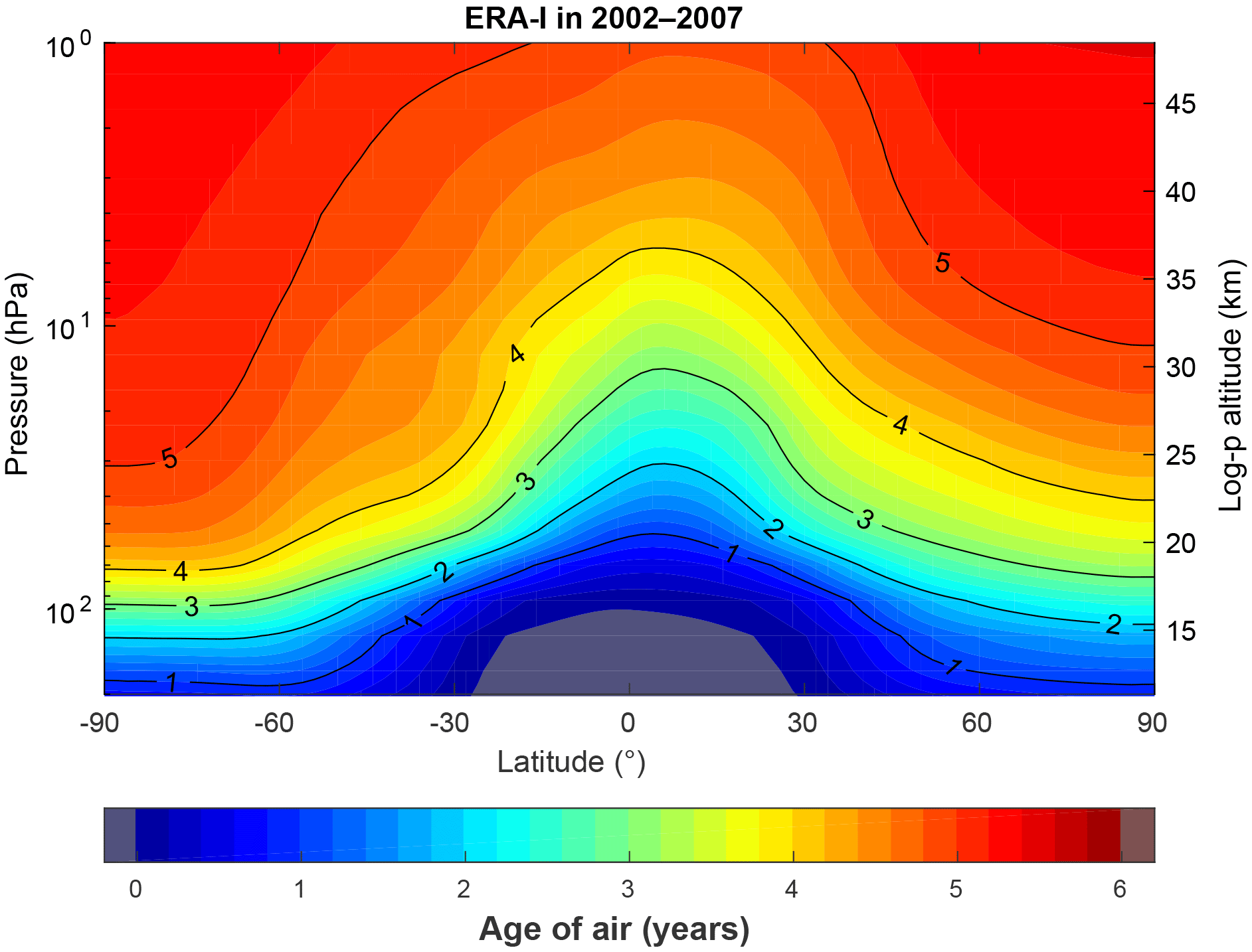
Figure 2Latitude–pressure distribution of AoA in 2002–2007 from the BASCOE simulation driven by ERA-I.
The four other reanalyses deliver noticeably different distributions of AoA (Fig. 3). One can distinguish JRA-55 and CFSR as the “younger reanalyses”, with AoA not exceeding 5 years in the polar upper stratosphere, MERRA as the “older reanalysis”, with maximum AoA values as large as 6.5 years, and ERA-I with intermediate results (5.8 years in the same regions). MERRA-2 is a special case, with upper stratospheric values similar to those reached by ERA-I but quite different latitudinal gradients. The hemispheric asymmetry is more pronounced with ERA-I than with any other reanalysis, e.g., the 3- and 4-year isolines (JRA-55 and CFSR, respectively) or the 5-year isoline (MERRA-2 and MERRA) reach nearly the same level above the North Pole as above the South Pole. MERRA-2 stands out in the middle stratosphere with nearly vertical isolines, i.e., very small vertical gradients which are not supported by MIPAS observations (Haenel et al., 2015; Kovács et al., 2017).
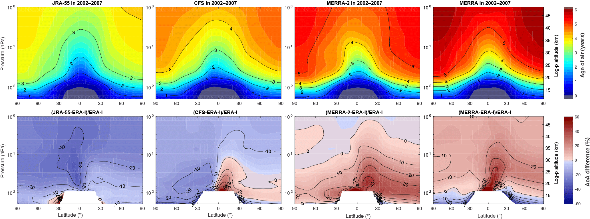
Figure 3Latitude–pressure distribution of AoA (years) in 2002–2007 from BASCOE simulations driven by all reanalyses but ERA-I (top row; same color scale as previous figure) and relative difference with respect to the mean AoA by the ERA-I-driven simulation for the same period (bottom row; difference is not plotted at grid points where ERA-I AoA is smaller than 5 days). These reanalyses are, from left to right, JRA-55, CFSR, MERRA-2 and MERRA.
While this qualitative comparison of the AoA distributions points to different gradients in the midlatitudes and polar regions, the relative differences with respect to ERA-I are largest in the tropical lower stratosphere (bottom row of Fig. 3). Hence, we focus on this region and its differences with the midlatitudes. Figure 4, inspired by the AoA intercomparisons in CCMs (Chipperfield et al., 2014; Neu et al., 2010), shows the intercomparison of AoA zonal means at 50 hPa, at tropical and northern midlatitudes, and the AoA difference between these two latitude bands.
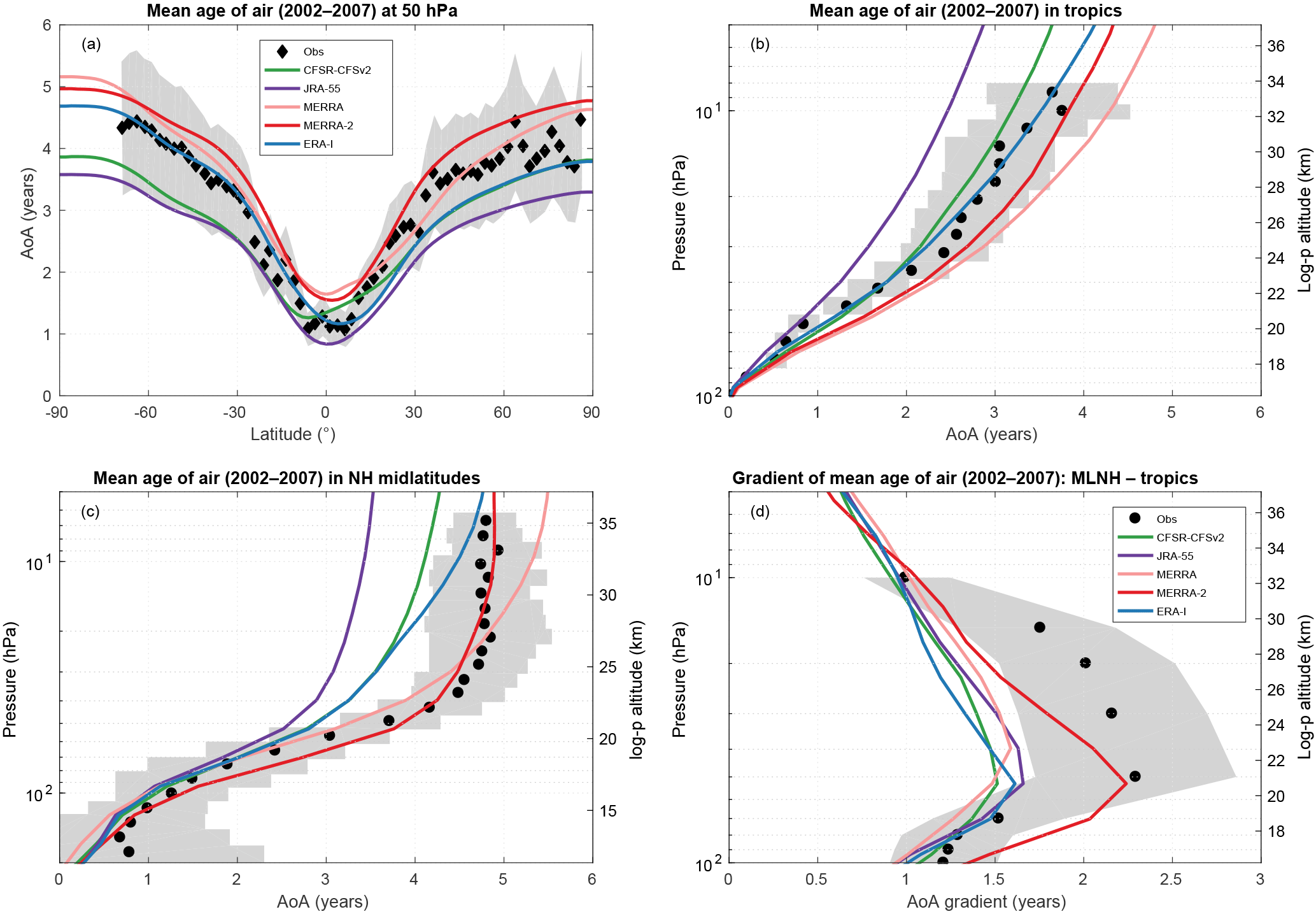
Figure 4AoA (years) in 2002–2007 by the BASCOE TM driven by five reanalyses (solid lines) versus in situ observations (symbols) with their 1σ uncertainties (grey shading). The five reanalyses are ERA-I (blue), MERRA-2 (red), MERRA (pink), JRA-55 (purple) and CFSR (green). (a) AoA at 50 hPa with aircraft observations of CO2 (Andrews et al., 2001; Neu et al., 2010). (b) AoA in the tropics (10∘ N–10∘ S) with aircraft observations (Andrews et al., 2001; Chipperfield et al., 2014). (c) AoA in the northern midlatitudes (35–45∘ N) with balloon observations (Chipperfield et al., 2014; Engel et al., 2009). (d) AoA differences between the northern midlatitudes and tropics (Chipperfield et al., 2014; Neu et al., 2010). The legend in panel (d) applies to panels (b) and (c) as well.
The intercomparison at 50 hPa (Fig. 4a) shows again the important disagreement between the five model simulations. JRA-55 yields the youngest AoA at all latitudes with values ranging from 0.8 years at the Equator to 3.6 years at the South Pole, while MERRA and MERRA-2 yield the oldest AoA with 1.6 years at the Equator and around 5 years at the South Pole. CFSR and ERA-I yield intermediate results with nearly identical values in the northern extratropics but different latitude gradients between the tropics and Southern Hemisphere. The sole simulation to deliver a minimum AoA in the southern tropics is driven by CFSR, which yields the minimum AoA at 6∘ S. In the other simulations, this minimum is either exactly at the Equator (JRA-55, MERRA) or slightly north of the Equator (ERA-I, MERRA-2). In the Southern Hemisphere, CFSR results in AoA nearly as young as JRA-55, while ERA-I reaches larger values which are very close to the observations. Overall, the spread between the five simulations at 50 hPa is larger than the 1σ observational uncertainties in the tropics and nearly as large in the extratropics. Since the reanalyses are constrained by very similar satellite datasets, they could have been expected to deliver more similar AoA than an intercomparison of unconstrained climate models. Yet we note that the spread shown in Fig. 4a is as large as in an intercomparison of seven CCMs (Chipperfield et al., 2014).
The vertical profiles of AoA (Fig. 4b and c) confirm that this large spread and general hierarchy of AoA (youngest with JRA-55, oldest with MERRA and MERRA-2) are found at all stratospheric levels. In the northern midlatitudes (35–45∘ N, Fig. 4c) MERRA-2 stands out with vertical gradients which are larger in the lower stratosphere but smaller in the upper stratosphere than in all other reanalyses. While the intermediate values by ERA-I and CFSR agree well with observations in the tropics (10∘ S–10∘ N, Fig. 4b), this is not the case in the northern midlatitudes, where only MERRA and MERRA-2 deliver AoA as old as the observations.
The AoA differences between the tropics and midlatitudes are directly related to the inverse of the tropical upwelling velocity and independent of quasi-horizontal mixing: a smaller AoA latitudinal gradient indicates faster tropical ascent (Linz et al., 2016; Neu and Plumb, 1999). These “latitudinal gradients of AoA” were used in several CCM intercomparisons (Chipperfield et al., 2014; Neu et al., 2010). Figure 4d shows this diagnostic for the five reanalyses, i.e., the differences between the AoA profiles in Fig. 4c and b. Except for MERRA-2, the profiles of AoA differences delivered by the four other reanalyses agree much more closely than the AoA profiles themselves, at least during the 2002–2007 period. The spread of AoA differences between the four reanalyses reaches a maximum of 0.2 years at 30 hPa, much tighter than the spread of 0.8 years in the corresponding intercomparison of six CCMs (Chipperfield et al., 2014). While there is good agreement with the observation-derived AoA differences below 60 and at 10 hPa, these four reanalyses significantly underestimate it at intermediate pressure levels. This indicates an overestimation of the tropical upwelling obtained with ERA-I, CFSR, JRA-55 and MERRA in the lower stratosphere. MERRA and MERRA-2 yield larger AoA at northern midlatitudes than the three other reanalyses. In the case of MERRA-2, this results in a profile of AoA differences which are significantly larger than the profiles obtained with the four other reanalyses but agrees much better with the profile derived from the observations. Hence, MERRA-2 apparently underestimates the tropical upwelling in the lowermost stratosphere (100–60 hPa), agrees better with the observations at 50 hPa than the four other reanalyses and is in accordance with them at higher levels.
3.2 Time evolution and absence of volcanic impact
The Pinatubo eruption, which started on 15 June 1991, is expected to have had a significant impact on AoA (Diallo et al., 2017; Muthers et al., 2016). The assimilation of satellite radiance measurements by the Advanced Microwave Sounding Unit (AMSU) started in 1998 (on 1 August in ERA-I and JRA-55, and 1 November in CFSR, MERRA and MERRA-2) and was repeatedly shown to have a important influence on their description of the stratospheric dynamics (Kawatani et al., 2016; Long et al., 2017; Simmons et al., 2014). Hence, we repeat the latitudinal gradient diagnostic but for the period 1992–1997, i.e., after the Pinatubo eruption and before the ingestion of AMSU radiances (Fig. 5). The general outcome is the same as during the later period: the tropical ascent is too fast with all reanalyses except with MERRA-2. Yet MERRA-2 provides a better match with the observations during this earlier period, and the four other reanalyses do not agree as closely.
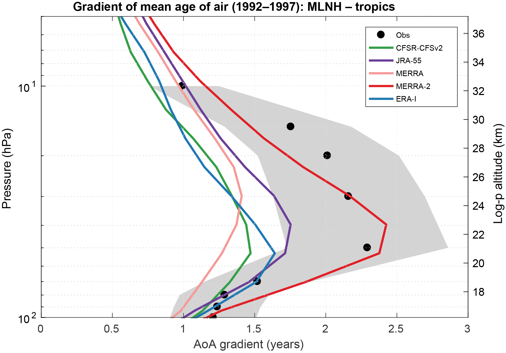
Figure 6 shows the averaged time evolution of simulated AoA according to the five reanalyses, from 1989 to 2015 at 50 hPa in the midlatitudes. The results are smoothed with a 1-year running mean in order to highlight the long-term trends. The overall hierarchy of ages shown on previous figures for years 2002–2007 holds for the whole 1989–2015 period: MERRA and MERRA-2 deliver the oldest AoA, JRA-55 and CFSR the youngest. While MERRA and MERRA-2 agree well in the Southern Hemisphere, this is not the case in the Northern Hemisphere, where MERRA-2 starts with much older values. A rapid decrease of MERRA-2 values during the 1990s allows these two datasets to reach better agreement after 1998, i.e., the beginning of AMSU assimilation. The possible causes for this apparently anomalous behavior of MERRA-2 will be discussed in Sect. 5. The MERRA output in the Northern Hemisphere delivers seasonal cycles with much larger amplitudes than those obtained from all other reanalyses. This will be investigated in the next section.
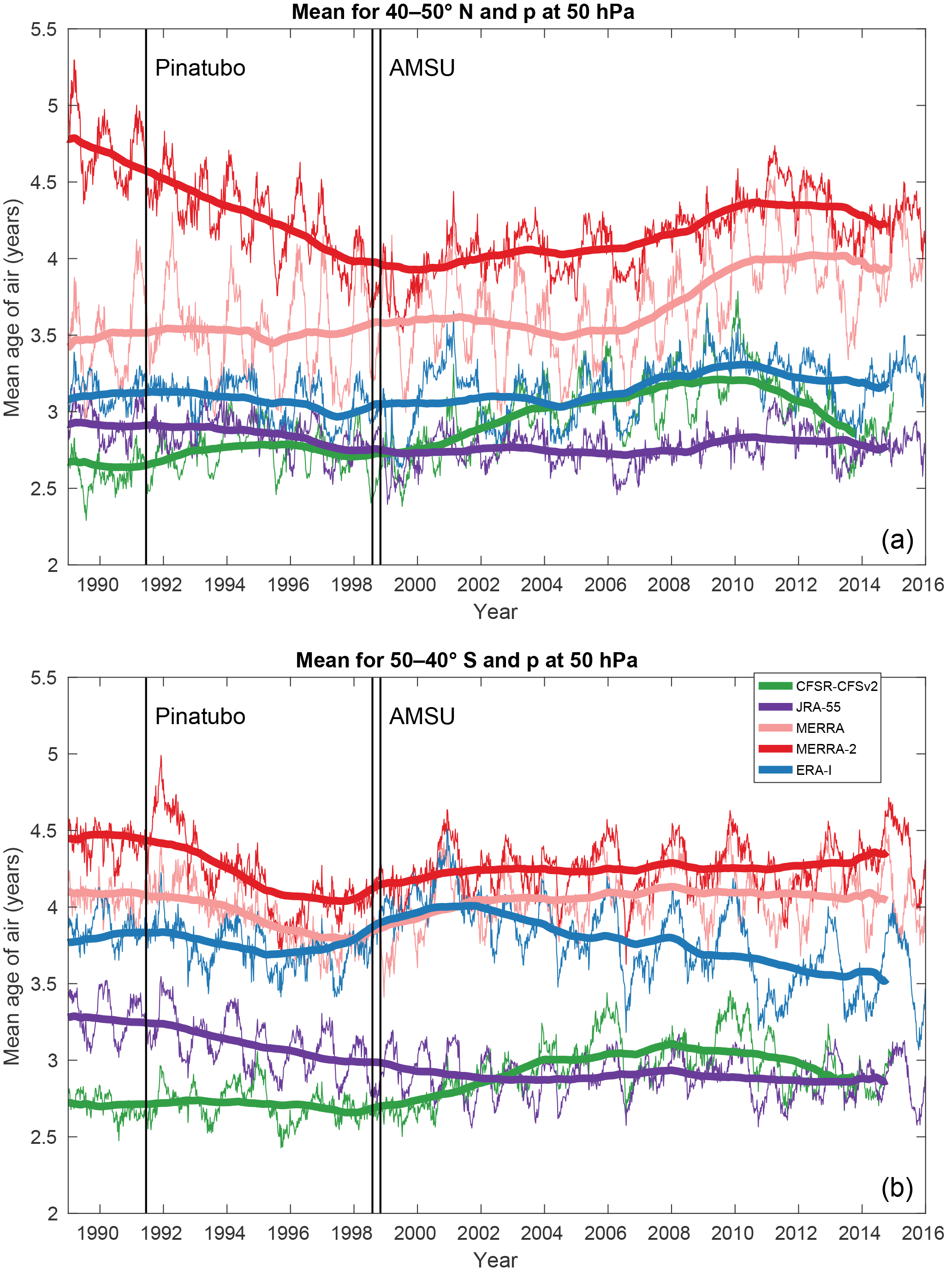
Figure 6Time evolution of AoA (years) interpolated to a pressure of 50 hPa in the northern midlatitudes (40–50∘ N mean, a) and in the southern midlatitudes (50–40∘ S mean, b). Thin lines show instantaneous model output every 5 days using the five reanalyses with color codes according the legend shown in the lower panel. Thick lines are smoothed with a 1-year running mean. The black vertical lines highlight the start of the Pinatubo eruption and the first assimilation of AMSU (see text).
The Pinatubo eruption does not appear to have any impact on the simulated AoA at 50 hPa except with MERRA-2 which shows an increase in the southern midlatitudes. The same time series for the tropical latitude band (30∘ S–30∘ N) does not show any impact of the Pinatubo eruption either (not shown). This absence of volcanic impact in the other reanalyses is even more evident in a deseasonalized time series of the extrapolar lower stratosphere (Fig. 7). This diagnostic is inspired by Diallo et al. (2017), who showed a significant impact of the Pinatubo eruption on AoA using ERA-I and JRA-55 but with another offline transport model. Since our results contradict this finding, this issue will also be further discussed in Sect. 5.
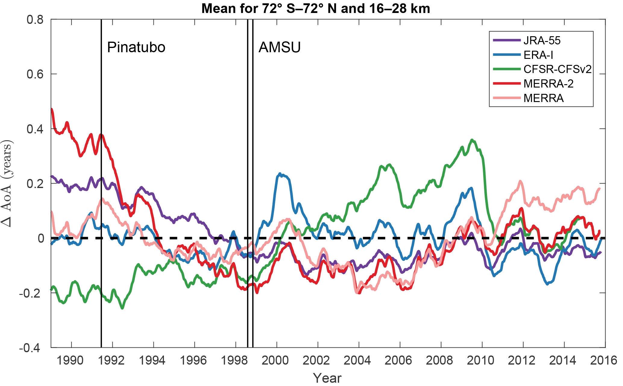
Figure 7Time evolution of the globally averaged (72∘ S–72∘ N) anomalies of AoA (years) with respect to their mean (1989–2015) annual cycles, between 16 and 28 km, using the five reanalyses with the same color codes as in previous figure.
Figure 8 displays time series of AoA in the middle stratosphere (mean values between 30 and 5 hPa). The left plot compares the model results in the Northern Hemisphere with balloon observations that have been collected since the 1970s (Engel et al., 2017), where the derivation of AoA uses the surface as reference and the outer error bars denote the overall uncertainty of the mean-age value including an assessment of the representativeness of a single profile (Engel et al., 2009). To allow a consistent comparison, the solid lines in Fig. 8 show modeled AoA using the surface as reference, i.e., AoA evaluated from a tracer which uses as boundary condition a global constant increasing linearly with time at the surface. This boundary condition is propagated to the free troposphere through vertical diffusion with a coefficient Kzz decreasing from an arbitrary value of 10 m2 s−1 at the surface to zero at the pressure level halfway between the surface and the tropopause. Figure 8b compares the resulting time series in the tropics with the usual calculation of AoA using the tropical tropopause as reference (dashed lines). The differences between the two calculations represent the transit times from the surface to the tropical tropopause, are nearly independent of the simulated year and range between 3 months (with ERA-I or JRA-55) and 6 months (with MERRA). These values are close to the longest transit times reported in a recent intercomparison of global models (Krol et al., 2018) indicating slow transport from the surface to the tropical tropopause which we attribute to the omission of deep convective transport in our model. While the surface-based model AoA (solid lines in Fig. 8) may be slightly overestimated, these biases have no significant interannual variations and do not hinder the intercomparison between reanalyses.
The spread between the five simulations is as large as the observational uncertainties, highlighting again the importance of the disagreement between the five reanalyses. In the northern midlatitudes (Fig. 8a), no reanalysis delivers any change larger than half a year over the whole period (1989–2015) except for MERRA-2 which indicates a large decrease of 0.8 years, but this decrease starts from values much larger than the observations and happens mostly before 2000. ERA-I delivers a weakly positive trend over the period 1989–2015, and we will assess in Sect. 4.3 that this trend in the model results is significant. While the overall trend simulated with ERA-I is in agreement with the balloon observations, this comparison should be considered with great caution because the sign of the AoA trend is not significant in the observations (Engel et al., 2009, 2017) and modeled trends over periods as long as 30 years are often not significant when the ideal tracer is sampled like the available observations of stratospheric tracers (Garcia et al., 2011).
The intercomparison in the Southern Hemisphere (Fig. 8c) also shows large disagreement between the long-term trends among the five reanalyses. MERRA and MERRA-2 values decrease quickly until 1995 and increase after 2007, while ERA-I values follow an opposite pattern. The long-term evolution of AoA in this region is completely different from JRA-55 (gradual decrease until 2002 followed by a stabilization) and differs yet again from CFSR (no apparent trend before 1997 and rapid increase during 1997–2003). The thin lines allow a qualitative comparison of faster variations. The seasonal signal dominates in all cases, with similar phases: AoA is oldest in fall and youngest in spring. The seasonal amplitudes are very dependent on the input reanalysis and on the considered year, so their detailed analysis is deferred to the next section. Yet we note already that some reanalyses exhibit a strong modulation of the seasonal cycle by the quasi-biennial oscillation (Baldwin et al., 2001), while others do not. This can be seen very clearly during the period 2005–2009 when the seasonal amplitudes of AoA by ERA-I and MERRA are approximately twice as small during the easterly phase of the QBO (i.e., in 2006 and 2008) than during the westerly phase (i.e., in 2005, 2007, 2009). This modulation of the seasonal variations is weaker in the MERRA-2 and JRA-55 datasets and absent from the CFSR dataset.
We now perform a quantitative investigation of the temporal variations in order to derive the amplitudes of periodic variations and the linear trends of AoA at all latitudes and pressure levels, including their uncertainties.
4.1 Methodology
Vigouroux et al. (2015) used a multiple linear regression model to study the trends of ozone total columns and vertical distribution at several ground-based stations. Here, we apply the same tool to A(t), the monthly zonal means of AoA as a function of time, latitude and pressure (after interpolation to a constant log-pressure grid with 2 km increments). The multiple linear regression model is expressed as
where t is time, A0 is the baseline value, A1 is the annual trend of AoA, and ϵ(t) represents the residuals. The term S(t) describes the seasonal variations in A(t):
where the coefficients S1 to S4 describe the seasonal cycle. The term Q(t) describes the variations due to the QBO and its seasonal modulations:
where the explanatory variables Q10(t) and Q30(t) are the zonal winds observed above Singapore at 10 and 30 hPa (data from the FU Berlin: http://www.geo.fu-berlin.de/en/met/ag/strat/produkte/qbo/index.html, last access: 10 October 2018), and Q1 to Q10 are the coefficients associated with these two proxies, including their seasonal dependence.
The uncertainties arising from the fit are calculated for the 95 % confidence interval and corrected for autocorrelation in the residuals (Santer et al., 2000). Preliminary tests also included additional terms to account for the El Niño–Southern Oscillation (ENSO), the 11-year solar cycle and volcanic forcings but it was found that these terms do not impact significantly the linear trends nor the amplitudes of seasonal and quasi-biennial oscillations. Hence, they were removed from the regression model in order to avoid any overfitting of the data and to ease the interpretation of the results.
An important goal of this analysis is the determination of linear trends. As seen in Figs. 6 and 8, such trends depend closely on the considered time period. Hence, the regression model was applied not only to the whole simulation period (1989–2015) but also to an “early period” (1989–2001) and a “recent period” (2002–2015) which start after the assimilation of AMSU and on the same year as the MIPAS mission (Stiller et al., 2008, 2012).
4.2 Amplitudes of the seasonal cycle and quasi-biennial oscillation
The amplitude of the seasonal variations is approximated by the difference between the maximum and minimum values reached by the term S(t) in the linear regression model. Figure 9 shows the dependence of this approximated amplitude with respect to pressure in five latitude bands for the period 2002–2015 (the results are similar for the period 1989–2001). The results with ERA-I are in agreement with an earlier modeling study (Diallo et al., 2012). The vertical structure agrees broadly across all five reanalyses in the extratropics with maximum amplitudes in the lower stratosphere (around 100 hPa), except above the South Pole, where the amplitudes are maximum in the middle stratosphere (10–30 hPa). MERRA and MERRA-2 stand out with larger amplitudes in the lower stratosphere, resulting above the South Pole in a secondary maximum which is not found by the three other reanalyses. One may argue that the larger seasonal amplitudes of MERRA and MERRA-2 are a direct consequence of their larger annual means (see Fig. 3) but this is not supported by the agreement of JRA-55 and CFSR with ERA-I despite their significantly younger annual means. In the tropics, ERA-I stands out with larger amplitudes in the upper stratosphere (around 5 hPa) and MERRA-2 with larger amplitudes in the lower stratosphere (around 50 hPa), while the three other reanalyses are in good agreement.
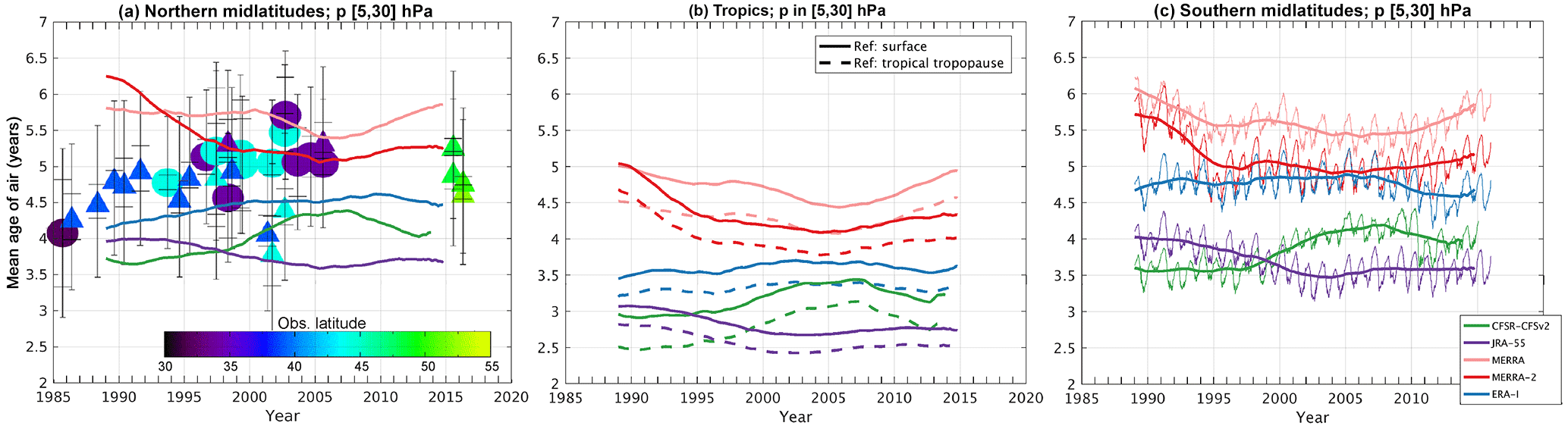
Figure 8 Time evolution of AoA (years) averaged from 30 to 5 hPa (approximately 24 to 36 km). Thick lines show model output smoothed with a 1-year running mean and line color codes as in previous figure. (a) Mean for the northern midlatitudes (40–50∘ N), where the symbols represent values derived from balloon observations of SF6 (circles) and CO2 (triangles) with color code showing the latitude of the measurements (according to the inset color bar) and outer error bars including sampling uncertainties (Engel et al., 2017). (b) Mean for the tropical latitudes (30∘ S–30∘ N), where the dashed lines show AoA using the tropical tropopause as reference. (c) Mean for the southern midlatitudes (50–40∘ S), where the thin lines show instantaneous model output every 5 days. Except for the dashed lines in panel (b), all AoA values in this figure use the surface as reference.
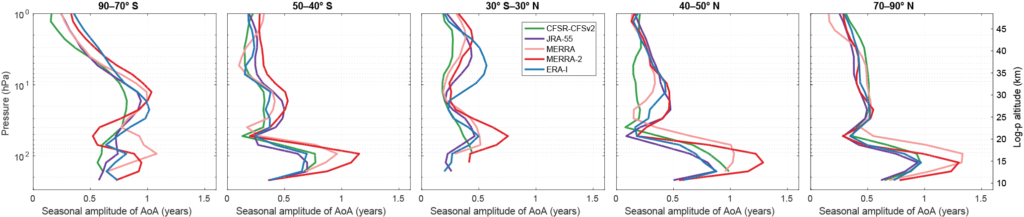
Figure 9 Amplitude (in years) of the seasonal variation in the 2002–2015 linear regression fit of AoA, as a function of pressure and averaged in five latitude bands, from left to right: North Pole (70–90∘ N); northern midlatitudes (40–50∘ N); tropics (30∘ S–30∘ N); southern midlatitudes (50–40∘ S); South Pole (90–70∘ S). The same color codes are used as in previous figures.
We now investigate the differences in the QBO among all reanalyses. Kawatani et al. (2016) have compared the monthly mean zonal wind in the equatorial stratosphere among reanalyses and found that their degree of disagreement depends on latitude, longitude, height and the phase of the QBO. They also noted a tendency for the agreement to be best near the longitude of Singapore, suggesting that the Singapore observations act as a strong constraint on all the reanalyses.
Here, we perform an intercomparison of the amplitude of the QBO signal (in years) in each reanalysis. We approximate it again as the difference between the maximum and minimum values reached by the term Q(t) in the linear regression model. Our results for ERA-I show that the QBO amplitude is largest in the subtropics around 30 hPa (not shown), which confirms again the results of Diallo et al. (2012). Figure 10 compares the results at this pressure level. Except for CFSR, the latitudinal dependence is similar in all reanalyses: the approximated QBO amplitude reaches maximum values around 15∘ latitude in both hemispheres and presents a marked minimum around the Equator. Outside of the equatorial region, the QBO amplitudes by JRA-55 are significantly smaller than by ERA-I, MERRA and MERRA-2. The amplitudes computed from CFSR show no clear structure in the Southern Hemisphere and reach large values at the North Pole.
4.3 Linear trends
It is difficult to infer changes in the BDC on the basis of AoA trends over periods shorter than several decades. Even in models where an ideal, linearly increasing artificial tracer is used, one has to rely on zonal-mean results over long periods to obtain trends that are clearly statistically significant (Garcia et al., 2011). The statement that is often made that climate models simulate a decreasing age throughout the stratosphere only applies over long time periods and is not necessarily the case for the past 25 years, when most tracer measurements were taken (Garfinkel et al., 2017). For example, the analysis of a 1700-year simulation showed that it takes around 30 years for a modeled BDC trend to emerge from the noise of natural climate variability (Hardiman et al., 2017).
While linear trends of AoA over shorter periods may represent transient changes due to climate variability, such changes over timescales which are intermediate between the QBO and the multidecadal scales are still relevant to the study of stratospheric dynamics. Current research on AoA trends has largely focused on a dipole-like latitudinal structure for the period 2002–2012, which was first derived from satellite observation of SF6 by the MIPAS instrument (Stiller et al., 2012). This structure of trends shows AoA decreasing in the Southern Hemisphere but increasing in the Northern Hemisphere, which was used to explain a recent increase of stratospheric HCl in the Northern Hemisphere (Mahieu et al., 2014) and interpreted as the consequence of a southward shift of the subtropical transport barriers (Stiller et al., 2017).
The ERA-I reanalysis supports a dipole-like latitudinal structure of AoA trends, at least since 2002. Haenel et al. (2015) derived AoA trends from the distribution of SF6 over the period 2002–2012, using MIPAS observations and a CCM nudged towards ERA-I below 1 hPa and found a good agreement for the signs, range and latitudinal structure of AoA trends (see Figs. 6 and 10 in H2015). Here, we aim to verify our methodology through a comparison of our results with H2015, to check the consistency of AoA trends derived from the four other reanalyses and to explore the latitudinal structure of AoA trends for periods starting earlier than 2002.
The linear trend is represented by A1 in the multiple regression linear model (Eq. 1). It is expressed in years per decade (yr dec−1) and is deemed significant at a given grid point if its absolute value is larger than its uncertainty (as defined in Sect. 4.1). Figure 11 presents the ERA-I trends during the period 2002–2012 in order to compare with H2015. In the polar regions, H2015 showed large and positive trends, while they are insignificant according to our model (Fig. 11). This disagreement can be attributed to different approaches: here, we study the true age of air using a theoretical tracer with no losses, while H2015 evaluated the apparent mean age of air taking into account the mesospheric sink of SF6 which has the largest impact in the polar regions (Reddmann et al., 2001). Outside of the polar regions, Fig. 11 shows good agreement with both observational and modeling results in H2015, including with respect to the significance of the trends: in the 30–60 hPa (approximately 25–20 km) layer the trends are significant at all extratropical latitudes, negative in the Southern Hemisphere and positive in the Northern Hemisphere. They reach −0.6 yr dec−1 in the southern tropics and close to 0.5 yr dec−1 in the northern tropics. Our results also agree well with those obtained by a diabatic model driven by ERA-I over the same period (Ploeger et al., 2015a).
Figure 12 compares the latitude–pressure distributions of AoA trends across all five reanalyses and for the early (1989–2001), recent (2002–2015) and overall periods (1989–2015). It is important to note that the trends over the early and overall periods should be considered with caution since there were little data to constrain the stratospheric winds until 1998 (see the discussion in the next section). The AoA trends derived from ERA-I wind fields during the early period (Fig. 12, upper left) grow in both hemispheres except for the northern lowermost stratosphere. During the recent period, the dipole structure derived from ERA-I (Fig. 12, upper middle) is similar than over the slightly shorter period 2002–2012 (Fig. 11). The increases in the Northern Hemisphere become weaker but remain significant at all latitudes, although at fewer grid points. The maximum trend is located at 24∘ N and 25 hPa, where it slightly exceeds 0.3±0.2 yr dec−1. The extension of this trend analysis for the overall period (Fig. 12, upper right) shows a dipole structure with negative but mostly insignificant trends in the Southern Hemisphere, positive trends in the northern middle stratosphere which mostly corresponds to the region with positive trends during the 1989–2001 period, and significantly negative trends in the lowermost stratosphere at all extrapolar latitudes. The same plot also shows that the positive trend which had been inferred visually for the northern midlatitudes of the middle stratosphere (Fig. 8a) is significant. Our ERA-I results for the overall period partly contradict those obtained by diabatic models which use not only the wind fields from ERA-I but also its heating rates (Diallo et al., 2012; Ploeger et al., 2015a). Looking at slightly shorter periods of two decades (1989–2010 for the former and 1990–2013 for the latter), these papers reported negative AoA trends for both hemispheres below 28 km altitude. Diallo et al. (2012) also looked at the middle stratosphere, where positive trends were found at all latitudes, suggesting that the shallow and deep Brewer–Dobson circulations may evolve in opposite directions.
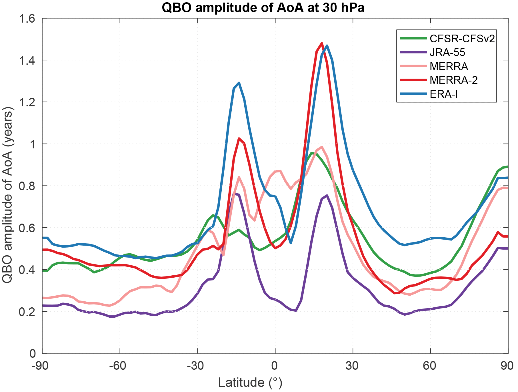
Figure 10 Amplitude (in years) of the QBO variation in the 2002–2015 linear regression fit of AoA, as a function of latitude at pressure 30 hPa. Same color codes as in previous figures.
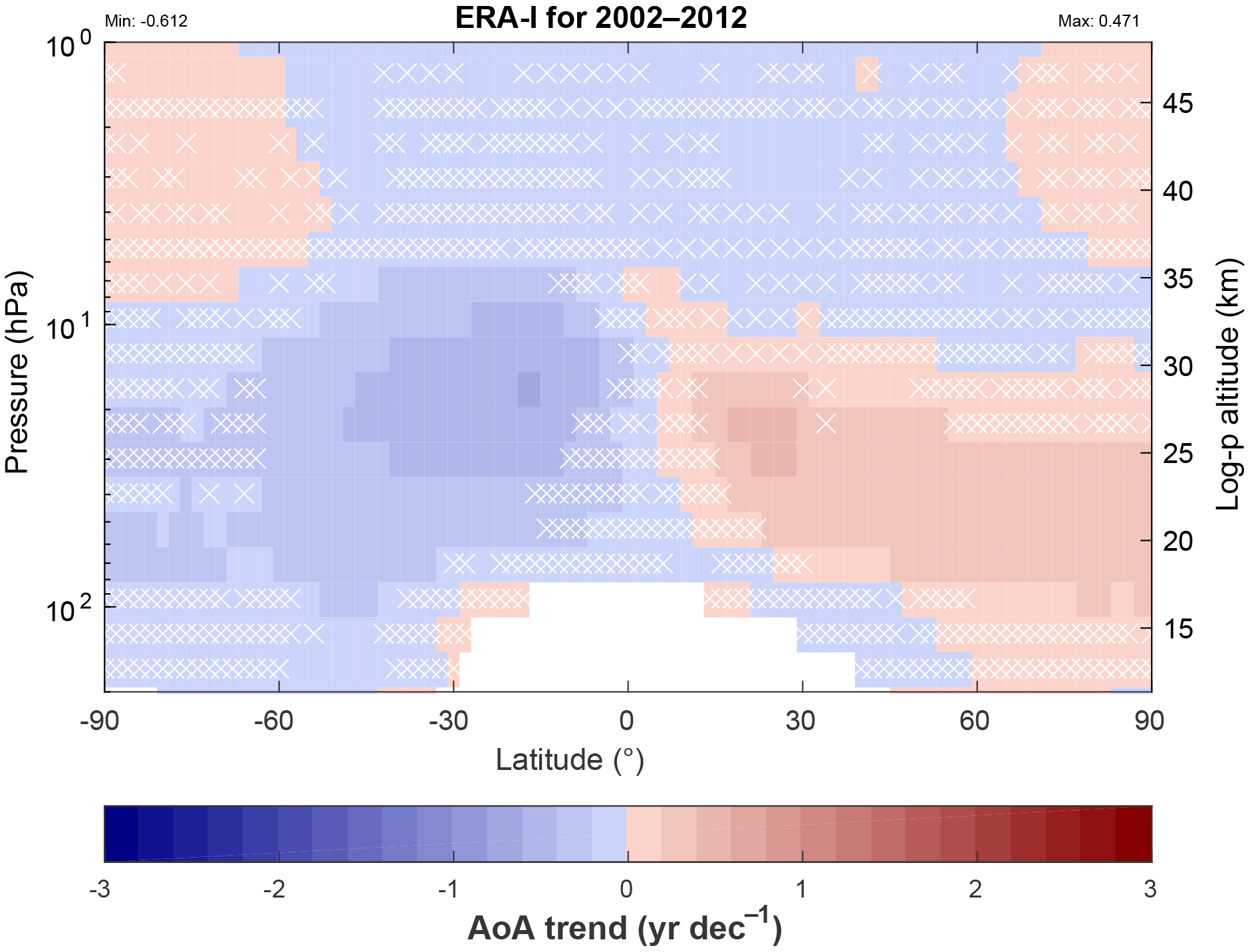
Figure 11Latitude–pressure distribution of AoA trends (in years per decade) using the ERA-Interim reanalysis over 2002–2012. White crosses indicate grid points where the sign of the trend is not significant; i.e., its absolute value is smaller than the uncertainty delivered by the regression analysis at the 95 % confidence level. The color scale is the same as in Haenel et al. (2015) with darker blues indicating more negative trends and darker reds more positive trends.
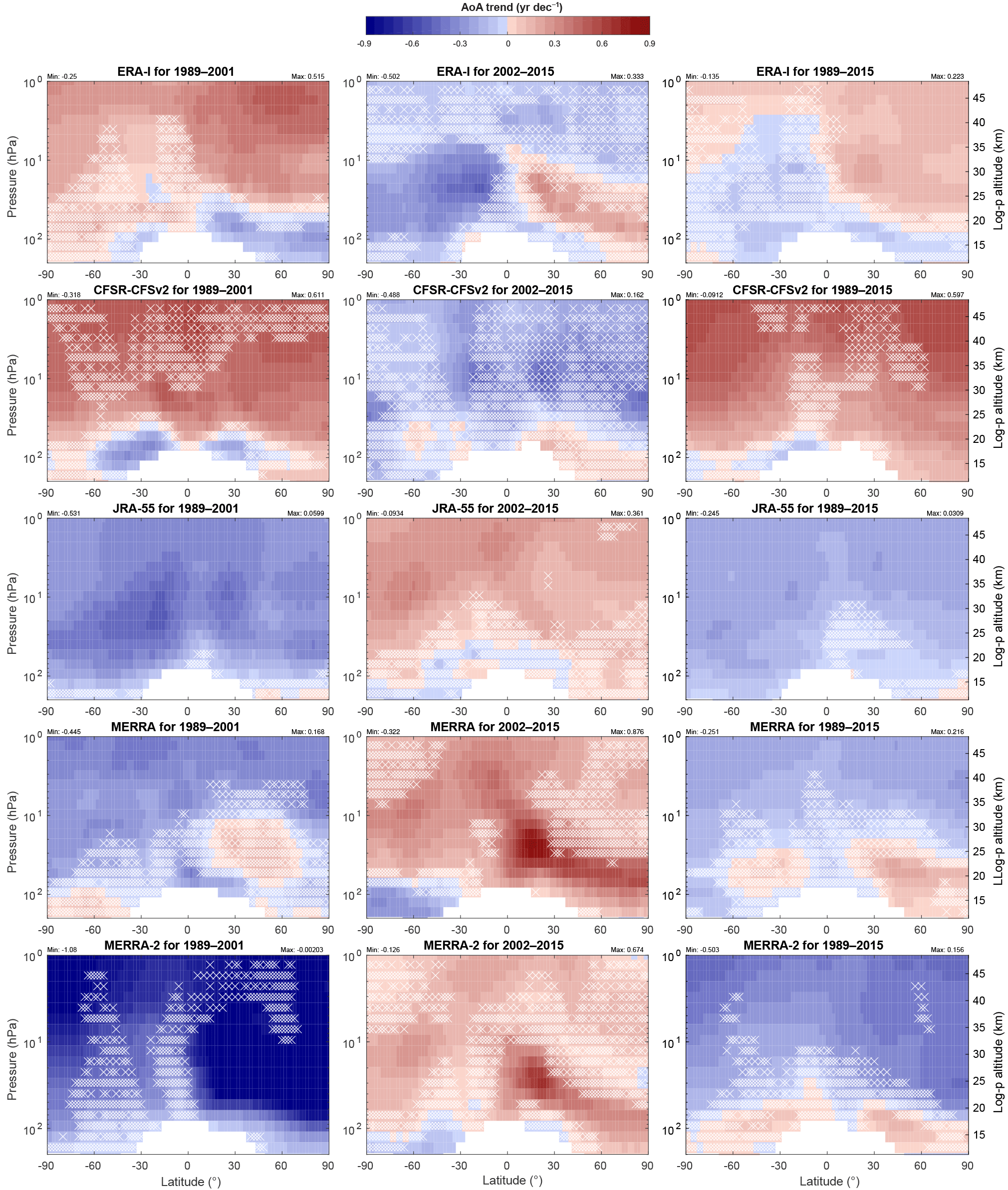
Figure 12Latitude–pressure distributions of AoA trends (in years per decade) over 1989–2001 (left column), 2002–2015 (middle column) and 1989–2015 (right column) using the five reanalyses (from top to bottom: ERA-I, CFSR, JRA-55, MERRA, MERRA-2). White crosses and colors have the same meaning as in the previous figure, but note the different scale (top of figure).
Comparing the results obtained with ERA-I with those from other reanalyses, one notes immediately general agreement between ERA-I and CFSR on one hand (Fig. 12, first and second row) and opposite trends in JRA-55, MERRA and MERRA-2 (third to fifth row). The agreement between multidecadal trends in ERA-I and CFSR may be related to their closeness in AoA distribution and spatial gradients (Sect. 3.1). For all reanalyses except ERA-I, the trends for the overall period (1989–2015; Fig. 12, right column) appear dominated by the results from the early period which are subject to caution.
To summarize, the signs of the trends depend strongly on the input reanalysis and on the considered period with values above 10 hPa varying between approximately −0.4 and 0.4 yr dec−1. JRA-55, MERRA and MERRA-2 indicate an AoA increasing globally over 2002–2015, except in the lowermost stratosphere, while ERA-I and CFSR indicate the opposite (Fig. 12, middle column). These trends are significant only in specific regions of the stratosphere, and the regions of significance vary depending on the considered reanalysis. ERA-I stands out as the only reanalysis yielding a dipole structure of AoA trends for the period 2002–2015, although one may note that, in the lower stratosphere, the AoA growth derived for this period from MERRA and MERRA-2 (Fig. 12, middle column, fourth and fifth row) is faster in the Northern Hemisphere than in the Southern Hemisphere. One notes also a reversal of the trends between the early (1989–2001) and recent (2002–2015) periods. This reversal is found for all five reanalyses and in all regions of the stratosphere but it is difficult to interpret because it goes in opposite directions in ERA-I and CFSR versus JRA-55, MERRA and MERRA-2.
The present intercomparison reveals large disagreement between the AoA derived from the five reanalyses, both with respect to their values and their linear trends. The spread of AoA at 50 hPa (Fig. 4a) is as large as in an intercomparison of CCMs (Chipperfield et al., 2014). An intercomparison of AoA trends during the 21st century among five CCMs shows negative trends in the whole middle atmosphere (about −0.05 yr dec−1) with no large hemispheric asymmetry (Butchart et al., 2010), while our results for 1989–2015 show faster changes (−0.4 to 0.4 yr dec−1) with different signs depending on the reanalysis and the stratospheric region. Since these results call for further research, we propose here a summary overview of the possible causes for this disagreement and some venues to attempt their identification.
Many intercomparisons of reanalyses have focused on the instantaneous values or long-term evolution of direct output fields such as temperature or zonal winds (Kozubek et al., 2017; Lawrence et al., 2015; Long et al., 2017; Simmons et al., 2014). These intercomparisons do not find large discrepancies, especially after the introduction of new satellite instruments around the year 2000. The large disagreement obtained here may be explained by the lack of wind observations available for assimilation in the tropics, high latitudes and stratosphere (Baker et al., 2014). This deficiency of wind information explains the divergences between trajectories obtained with different reanalyses in the lower stratosphere, e.g., in the equatorial region during some phases of the QBO (Podglajen et al., 2014) or above the Antarctic during the vortex break-up season (Hoffmann et al., 2017). Such divergent trajectories could have a significant cumulative impact on the mean age of air because it is a time-integrated diagnostic spanning several years.
Since the wind fields are weakly constrained, the causes for the disagreement found here may lie in the differences between the underlying models which were summarized recently in the context of S-RIP (Fujiwara et al., 2017). Let us first look at vertical resolution, which has an important impact on the modeling of lower stratospheric dynamics (Richter et al., 2014). In the lower stratosphere, the vertical resolution of CFSR is finest, while the resolution of and ERA-I and JRA-55 is the coarsest, with the resolution of MERRA and MERRA-2 in between (Fujiwara et al., 2017). This has no clear impact on AoA, since CFSR and JRA-55 deliver the youngest AoA, while MERRA and MERRA-2 deliver the oldest, with ERA-I results in between. Hence, one cannot establish a simple link between vertical resolution and AoA in this intercomparison.
The present intercomparison cannot establish the impact of different horizontal resolutions because it uses a common horizontal grid with a coarse resolution of (see Sect. 2.1 and 2.3). For example, the intercomparison of AoA distributions (Sect. 3.1) showed that JRA-55 and CFSR yield the weakest latitudinal gradients despite their horizontal grid spacing which is finest among the five reanalyses studied here (Fujiwara et al., 2017). Another intercomparison could yield different results if it uses the wind fields in each reanalysis at its original resolution – but this could lead to difficulties in the handling of horizontal diffusion (Jablonowski and Williamson, 2011).
Different parameterizations of gravity wave drag are another possible modeling cause for the disagreement in AoA. ERA-I, JRA-55 and CFSR all neglect non-orographic gravity wave drag (except for CFSv2, i.e., CFSR after 2010) and each uses its own parameterization of orographic gravity wave drag. MERRA and MERRA-2, on the other hand, use the same parameterization for orographic gravity wave drag (McFarlane, 1987) and both take non-orographic gravity wave drag into account.
Miyazaki et al. (2016) compared the mean-meridional circulations and also the mixing strengths in six reanalyses – including ERA-I and JRA-55 – and also found significant disagreement. Their diagnostics are closely related to AoA, since a faster mean-meridional circulation evidently leads to younger AoA and increased mixing corresponds mostly to additional aging of air due to recirculation from the extratropics to the tropics (Garny et al., 2014). For example, the disagreement of linear trends for 1989–2015 (right column in Fig. 12) confirms the finding that ERA-I and JRA-55 have opposite linear trends of tropical upward mass flux for the period 1979–2012, with fluxes increasing at all levels in JRA-55, while in ERA-I they increase only in a shallow layer of the lower troposphere but decrease in the middle stratosphere (Miyazaki et al., 2016). Similar disagreement has also been reported between the trends of the annual mean tropical upwelling in three reanalyses over the period 1979–2012, with vertical residual velocities () increasing in MERRA and JRA-55 and decreasing in ERA-I (Abalos et al., 2015).
MERRA-2 stands out with outlying AoA values during the 1990s. A connection is plausible with its difficulties representing correctly the QBO before 1995 (Coy et al., 2016; Kawatani et al., 2016). Gelaro et al. (2017) noted on that same year a marked decrease in temperature near 1 hPa and associated it with a change in assimilated radiance data. Gelaro et al. (2017) describe three features which are absent from the other reanalysis systems and could also play a role in the description of middle atmosphere dynamics in MERRA-2, contributing to its outlying AoA. With respect to assimilated observations, MERRA-2 is the only reanalysis to assimilate Microwave Limb Sounder on the Aura satellite (Aura-MLS) temperatures, from 2004 onwards and above 5 hPa. While this has an important impact on temperatures in the upper stratosphere and lower mesosphere, it does not seem to have an impact on the AoA time series in the middle stratosphere (Fig. 8) and cannot explain the large values obtained during the 1990s. With respect to forward model forcings, MERRA-2 is the only reanalysis which includes a large source of non-orographic gravity wave drag in the tropics (Molod et al., 2015) and realistic aerosol optical depths. This last feature most likely explains the sensitivity of the MERRA-2 AoA at 50 hPa to the Pinatubo eruption, which cannot be seen with any other reanalysis (Fig. 6).
Yet the impact of the Pinatubo eruption on MERRA-2 AoA at 50 hPa cannot be seen in the northern midlatitudes, and in the southern midlatitudes it is not larger than the amplitude of seasonal variations. In Sect. 3.2, we could not find any influence of volcanic aerosols at the global scale (Fig. 7), contrary to recent results obtained by Diallo et al. (2017) using the Chemical Lagrangian Model of the Stratosphere (CLaMS) driven by ERA-I and JRA-55. While CLaMS is a Lagrangian transport model including a mixing parameterization (Konopka et al., 2004) and BASCOE TM a Eulerian transport model, we suggest that these conflicting results are better explained by the different approaches with respect to vertical transport: BASCOE TM is a kinematic model (see Sect. 2.1), while CLaMS is a diabatic transport model and hence also driven by the heating rates from the reanalysis forecast models (Ploeger et al., 2010, 2015b).
Wright and Fueglistaler (2013) have shown that the heat budgets differ significantly in the tropical tropopause layer among the reanalyses, with substantial implications for representations of transport and mixing in this region. Abalos et al. (2015) evaluated the vertical component of the advective BDC in ERA-I, MERRA and JRA-55, and found substantial differences between direct (i.e., kinematic) estimates and indirect estimates derived from the thermodynamic balance (i.e., using diabatic heating rates). These intercomparisons of dynamical diagnostics highlight the need for another intercomparison of AoA using a diabatic transport model, because this approach would also reflect the differences between the diabatic heat budgets of each reanalysis – including the temperature increments from the assimilation of temperature radiances (Diallo et al., 2017).
Future work will also involve the disentangling of the contributions to AoA of the residual circulation, mixing on resolved scales and mixing on unresolved scales (i.e., diffusion) as recently performed with ERA-I (Dietmüller et al., 2017; Ploeger et al., 2015a) and quantitative comparisons with observational datasets, using both MIPAS observations of SF6 (Haenel et al., 2015; Stiller et al., 2012) and balloon observations of SF6 and CO2 (Ray et al., 2014). Comparisons with long-term records of other long-lived tracers will provide further insight at multidecadal scales. A recent study by Douglass et al. (2017) explained that the relationship between AoA and the fractional release of such tracers is a stronger test of the realism of simulated transport than the simple comparisons of mean age distributions. This approach seems very promising not only in the context of S-RIP but also for observation-based evaluations of stratospheric transport in global circulation–chemistry models.
We have developed a preprocessor to feed a Eulerian and kinematic transport model with any of the available global reanalysis datasets. This has allowed us to compute the mean AoA in the stratosphere and its evolution from 1985 to 2015, according to five modern reanalyses: ERA-Interim, JRA-55, MERRA, MERRA-2 and CFSR. Our results compare well with those published previously using other transport models driven by ERA-Interim and MERRA-2.
The five reanalyses deliver very different and diverse results. In the middle and upper stratosphere, MERRA yields the oldest AoA (∼5–6 years at midlatitudes) and JRA-55 the youngest one (∼3.5 years). MERRA-2 provides a different distribution of latitudinal and vertical AoA gradients than any other reanalysis, with near-zero vertical gradients in the middle stratosphere which are not supported by observations. CFSR and ERA-I give the most similar AoA distributions, with the latter providing stronger gradients vertically in the middle stratosphere and latitudinally in the Southern Hemisphere. The relative differences between ERA-I and the four other reanalyses are largest in the lower tropical stratosphere. Tropical ascent rates have been compared through the difference between AoA in the northern midlatitudes and in the tropics, showing good agreement between all reanalyses except for MERRA-2 and an overestimation of the upwelling in the tropical lower stratosphere.
The time variations of AoA were studied first through a qualitative analysis of raw time series in the midlatitudes, then through a fit with a multiple linear regression model. While the linear trends vary considerably depending on the considered period (2002–2012, 2002–2015 or 1985–2015), the general hierarchy of older (MERRA, MERRA-2) and younger (JRA-55, CFSR) reanalyses holds during the whole 1985–2015 period, with ERA-I keeping intermediate AoA values. The MERRA-2 results stand out again, with an exceptionally large initial AoA in the Northern Hemisphere which quickly decreases during the 1990s to reach values similar to those in MERRA. A comparison was performed with a time series of balloon observations realized since the 1970s in the northern midlatitudes, where the uncertainties include an evaluation of the sampling error (Engel et al., 2017). The spread between the five simulations is as large as the observational uncertainties, highlighting again the importance of the disagreement between the five reanalyses.
The amplitudes of seasonal variations agree broadly across all five reanalyses but in the lower stratosphere they are larger in MERRA and MERRA-2 than in the three other reanalyses. The latitudinal dependence of QBO amplitudes is similar in all five reanalyses except for CFSR which shows no clear structure in the Southern Hemisphere.
The linear trends of ERA-I AoA confirm again the dipole structure of the latitude–height distribution of AoA trends as derived from MIPAS observations of SF6 for the 2002–2012 period (Haenel et al., 2015), with a decrease in the Southern Hemisphere reaching about −0.6 yr dec−1 and an increase in the northern lower stratosphere reaching about 0.5 yr dec−1. The increase in the Northern Hemisphere is significant (at the 95 % confidence level) and it is not obtained in multidecadal climate model simulations. Yet the trends derived from ERA-I are shown to closely depend on the considered period. When it is extended to 2002–2015, the positive trends in the Northern Hemisphere become weaker (about 0.3 yr dec−1) and they are significant at fewer grid points. A further extension to 1989–2015 shows that the negative trends in the southern middle stratosphere become insignificant. For all five reanalyses, the trends over the early period (1989–2001) have opposite signs compared to over the recent period (2002–2015). Looking only at the recent period which is better constrained by observations, the main outcome is again large disagreement between the reanalyses: JRA-55, MERRA and MERRA-2 provide increasing AoA in the middle stratosphere, while CFSR provides a decreasing but mostly insignificant trend. To summarize, the signs of the trends depend strongly on the input reanalysis and on the considered period with values above 10 hPa varying between approximately −0.4 and 0.4 yr dec−1. Independently of the considered period, no reanalysis other than ERA-I finds any dipole structure in the latitude–height distribution of AoA trends.
Since the wind fields are weakly constrained, the causes for the disagreement found here may lie in the differences between the underlying models. While no obvious cause could be found, we suggest that the parameterization of non-orographic gravity wave drag deserves further investigation, especially in the case of MERRA-2, which has difficulties representing correctly the QBO before 1995. No global impact of the Pinatubo eruption can be found in our simulations of AoA, contrary to a recent study which used ERA-I and JRA-55 to drive a diabatic transport model. This highlights the need to repeat the present intercomparison with diabatic transport models because they would reflect directly the significant differences between the heating rates in the reanalyses (Wright and Fueglistaler, 2013). Future work will also focus on quantitative comparisons with AoA derived from MIPAS observations of SF6, comparisons with the long-term records of other long-lived tracers to provide further insight at multidecadal scales, and disentangling the contributions to AoA of residual circulation, mixing on resolved scales and mixing on unresolved scales.
The main conclusion of this study is the significant diversity in the distribution of mean AoA which we obtain with our transport model, depending on the input reanalysis. This casts doubt on our ability to model accurately the time necessary for variations of greenhouse or ozone-depleting species to propagate from the troposphere to the stratosphere. We have also found large disagreement between the five reanalyses with respect to the long-term trends of age of air. This suggests that with our type of offline transport model, the wind fields in modern reanalyses are not sufficiently constrained by observations to evaluate the actual changes of stratospheric circulation. Yet this conclusion should not be hastily extended to other types of transport models which also use the reanalyses of temperature and heating rates.
The monthly zonal averages of AoA, as delivered by the BASCOE TM experiments driven by the five input reanalyses, are distributed as the Supplement to this article. The source code of the BASCOE TM, including its tools to preprocess the reanalyses, is available by email request to the corresponding author. The ERA-Interim reanalysis (Dee et al., 2011) is provided by the ECMWF; see http://apps.ecmwf.int/datasets/data/interim-full-daily (last access: 10 October 2018). MERRA data (GMAO, 2008) and MERRA-2 data (GMAO, 2015) are provided by the Global Modeling and Assimilation Office at NASA Goddard Space Flight Center through the NASA GES DISC online archive. The CFSR (Saha et al., 2010b) and CFSv2 (Saha et al., 2011) reanalyses data were obtained from NOAA. The JRA-55 reanalysis (JMA, 2013) was obtained from the NCAR Research Data Archive.
The supplement related to this article is available online at: https://doi.org/10.5194/acp-18-14715-2018-supplement.
SC designed the study and wrote the paper. CV performed the multiple linear regression analysis. YC, QE, DM, BMMS and AS contributed to data preprocessing, model development and validation. AE provided the observational balloon dataset. EM provided advice and insights during the course of the study. All co-authors contributed to the interpretation of the results and the reviews of the draft manuscripts.
The authors declare that they have no conflict of interest.
This article is part of the special issue “The SPARC Reanalysis Intercomparison Project (S-RIP) (ACP/ESSD inter-journal SI)”. It is not associated with a conference.
We thank the reanalysis centers (ECMWF, NASA GSFC, NOAA NCEP and JMA) for
providing their support and data products. We thank Gabriele Stiller, Paul
Konopka and Bernard Legras for fruitful discussions during the preliminary
steps leading to this study and Masatomo Fujiwara for his coordination of
the S-RIP. We would also like to thank the editor and two anonymous reviewers
for their valuable comments. Yves Christophe's contribution was partly
supported by the European Commission project MACC-II under the EU Seventh
Research Framework Programme (contract no. 283576). Daniele Minganti's
contribution was financially supported by the Fonds de la Rechecherce
Fondamentale Collective through research project ACCROSS (convention
PDRT.0040.16). Emmanuel Mahieu is a research associate with the F.R.S.-FNRS.
Edited by: William Lahoz
Reviewed by: two anonymous referees
Abalos, M., Legras, B., Ploeger, F., and Randel, W. J.: Evaluating the advective Brewer-Dobson circulation in three reanalyses for the period 1979–2012, J. Geophys. Res.-Atmos., 120, 7534–7554, https://doi.org/10.1002/2015JD023182, 2015. a, b
Andrews, A. E., Boering, K. A., Daube, B. C., Wofsy, S. C., Loewenstein, M., Jost, H., Podolske, J. R., Webster, C. R., Herman, R. L., Scott, D. C., Flesch, G. J., Moyer, E. J., Elkins, J. W., Dutton, G. S., Hurst, D. F., Moore, F. L., Ray, E. A., Romashkin, P. A., and Strahan, S. E.: Mean ages of stratospheric air derived from in situ observations of CO2, CH4, and N2O, J. Geophys. Res., 106, 32295–32314, https://doi.org/10.1029/2001JD000465, 2001. a, b, c
Austin, J. and Li, F.: On the relationship between the strength of the Brewer-Dobson circulation and the age of stratospheric air, Geophys. Res. Lett., 33, l17807, https://doi.org/10.1029/2006GL026867, 2006. a
Baker, W. E., Atlas, R., Cardinali, C., Clement, A., Emmitt, G. D., Gentry, B. M., Hardesty, R. M., Källén, E., Kavaya, M. J., Langland, R., Ma, Z., Masutani, M., McCarty, W., Pierce, R. B., Pu, Z., Riishojgaard, L. P., Ryan, J., Tucker, S., Weissmann, M., and Yoe, J. G.: Lidar-Measured Wind Profiles: The Missing Link in the Global Observing System, B. Am. Meteorol. Soc., 95, 543–564, https://doi.org/10.1175/BAMS-D-12-00164.1, 2014. a
Baldwin, M. P., Gray, L. J., Dunkerton, T. J., Hamilton, K., Haynes, P. H., Randel, W. J., Holton, J. R., Alexander, M. J., Hirota, I., Horinouchi, T., Jones, D. B. A., Kinnersley, J. S., Marquardt, C., Sato, K., and Takahashi, M.: The quasi-biennial oscillation, Rev. Geophys., 39, 179–229, https://doi.org/10.1029/1999RG000073, 2001. a
Bengtsson, L. and Shukla, J.: Integration of Space and In Situ Observations to Study Global Climate Change, B. Am. Meteorol. Soc., 69, 1130–1143, https://doi.org/10.1175/1520-0477(1988)069<1130:IOSAIS>2.0.CO;2, 1988. a
Bloom, S., Takacs, L., DaSilva, A., and Ledvina, D.: Data assimilation using incremental analysis updates, Mon. Weather Rev., 124, 1256–1271, 1996. a
Bregman, B., Segers, A., Krol, M., Meijer, E., and van Velthoven, P.: On the use of mass-conserving wind fields in chemistry-transport models, Atmos. Chem. Phys., 3, 447–457, https://doi.org/10.5194/acp-3-447-2003, 2003. a
Butchart, N.: The Brewer-Dobson circulation, Rev. Geophys., 52, 157–184, https://doi.org/10.1002/2013RG000448, 2014. a
Butchart, N., Cionni, I., Eyring, V., Shepherd, T. G., Waugh, D. W., Akiyoshi, H., Austin, J., Brühl, C., Chipperfield, M. P., Cordero, E., Dameris, M., Deckert, R., Dhomse, S., Frith, S. M., Garcia, R. R., Gettelman, A., Giorgetta, M. A., Kinnison, D. E., Li, F., Mancini, E., McLandress, C., Pawson, S., Pitari, G., Plummer, D. A., Rozanov, E., Sassi, F., Scinocca, J. F., Shibata, K., Steil, B., and Tian, W.: Chemistry–Climate Model Simulations of Twenty-First Century Stratospheric Climate and Circulation Changes, J. Climate, 23, 5349–5374, https://doi.org/10.1175/2010JCLI3404.1, 2010. a
Chipperfield, M. P.: New version of the TOMCAT/SLIMCAT off-line chemical transport model: Intercomparison of stratospheric tracer experiments, Q. J. Roy. Meteor. Soc., 132, 1179–1203, https://doi.org/10.1256/qj.05.51, 2006. a, b
Chipperfield, M. P., Liang, Q., Strahan, S. E., Morgenstern, O., Dhomse, S. S., Abraham, N. L., Archibald, A. T., Bekki, S., Braesicke, P., Di Genova, G., Fleming, E. L., Hardiman, S. C., Iachetti, D., Jackman, C. H., Kinnison, D. E., Marchand, M., Pitari, G., Pyle, J. A., Rozanov, E., Stenke, A., and Tummon, F.: Multimodel estimates of atmospheric lifetimes of long-lived ozone-depleting substances: Present and future, J. Geophys. Res., 119, 2555–2573, https://doi.org/10.1002/2013JD021097, 2014. a, b, c, d, e, f, g, h
Coy, L., Wargan, K., Molod, A. M., McCarty, W. R., and Pawson, S.: Structure and Dynamics of the Quasi-Biennial Oscillation in MERRA-2, J. Climate, 29, 5339–5354, https://doi.org/10.1175/JCLI-D-15-0809.1, 2016. a
Dee, D. P., Uppala, S. M., Simmons, A. J., Berrisford, P., Poli, P., Kobayashi, S., Andrae, U., Balmaseda, M. A., Balsamo, G., Bauer, P., Bechtold, P., Beljaars, A. C. M., van de Berg, L., Bidlot, J., Bormann, N., Delsol, C., Dragani, R., Fuentes, M., Geer, A. J., Haimberger, L., Healy, S. B., Hersbach, H., Hólm, E. V., Isaksen, L., Kållberg, P., Köhler, M., Matricardi, M., McNally, A. P., Monge-Sanz, B. M., Morcrette, J.-J., Park, B.-K., Peubey, C., de Rosnay, P., Tavolato, C., Thépaut, J.-N., and Vitart, F.: The ERA-Interim reanalysis: configuration and performance of the data assimilation system, Q. J. Roy Meteor. Soc., 137, 553–597, https://doi.org/10.1002/qj.828, 2011. a, b, c, d
Diallo, M., Legras, B., and Chédin, A.: Age of stratospheric air in the ERA-Interim, Atmos. Chem. Phys., 12, 12133–12154, https://doi.org/10.5194/acp-12-12133-2012, 2012. a, b, c, d, e
Diallo, M., Ploeger, F., Konopka, P., Birner, T., Müller, R., Riese, M., Garny, H., Legras, B., Ray, E., Berthet, G., and Jegou, F.: Significant Contributions of Volcanic Aerosols to Decadal Changes in the Stratospheric Circulation, Geophys. Res. Lett., 44, 10780–10791, https://doi.org/10.1002/2017GL074662, 2017. a, b, c, d
Dietmüller, S., Garny, H., Plöger, F., Jöckel, P., and Cai, D.: Effects of mixing on resolved and unresolved scales on stratospheric age of air, Atmos. Chem. Phys., 17, 7703–7719, https://doi.org/10.5194/acp-17-7703-2017, 2017. a
Douglass, A. R., Strahan, S. E., Oman, L. D., and Stolarski, R. S.: Multi-decadal records of stratospheric composition and their relationship to stratospheric circulation change, Atmos. Chem. Phys., 17, 12081–12096, https://doi.org/10.5194/acp-17-12081-2017, 2017. a
Engel, A., Mobius, T., Bonisch, H., , Schmidt, U., Heinz, R., Levin, I., Atlas, E., Aoki, S., Nakazawa, T., Sugawara, S., Moore, F., Hurst, D., Elkins, J., Schauffler, S., Andrews, A., and Boering, K.: Age of stratospheric air unchanged within uncertainties over the past 30 years, Nat. Geosci., 2, 28–31, https://doi.org/10.1038/ngeo388, 2009. a, b, c, d
Engel, A., Bönisch, H., Ullrich, M., Sitals, R., Membrive, O., Danis, F., and Crevoisier, C.: Mean age of stratospheric air derived from AirCore observations, Atmos. Chem. Phys., 17, 6825–6838, https://doi.org/10.5194/acp-17-6825-2017, 2017. a, b, c, d, e
Errera, Q., Daerden, F., Chabrillat, S., Lambert, J. C., Lahoz, W. A., Viscardy, S., Bonjean, S., and Fonteyn, D.: 4D-Var assimilation of MIPAS chemical observations: ozone and nitrogen dioxide analyses, Atmos. Chem. Phys., 8, 6169–6187, https://doi.org/10.5194/acp-8-6169-2008, 2008. a
Fu, Q., Lin, P., Solomon, S., and Hartmann, D. L.: Observational evidence of strengthening of the Brewer-Dobson circulation since 1980, J. Geophys. Res., 120, 10214–10228, https://doi.org/10.1002/2015JD023657, 2015. a
Fujiwara, M., Wright, J. S., Manney, G. L., Gray, L. J., Anstey, J., Birner, T., Davis, S., Gerber, E. P., Harvey, V. L., Hegglin, M. I., Homeyer, C. R., Knox, J. A., Krüger, K., Lambert, A., Long, C. S., Martineau, P., Molod, A., Monge-Sanz, B. M., Santee, M. L., Tegtmeier, S., Chabrillat, S., Tan, D. G. H., Jackson, D. R., Polavarapu, S., Compo, G. P., Dragani, R., Ebisuzaki, W., Harada, Y., Kobayashi, C., McCarty, W., Onogi, K., Pawson, S., Simmons, A., Wargan, K., Whitaker, J. S., and Zou, C.-Z.: Introduction to the SPARC Reanalysis Intercomparison Project (S-RIP) and overview of the reanalysis systems, Atmos. Chem. Phys., 17, 1417–1452, https://doi.org/10.5194/acp-17-1417-2017, 2017. a, b, c, d, e, f, g
Garcia, R. R., Randel, W. J., and Kinnison, D. E.: On the Determination of Age of Air Trends from Atmospheric Trace Species, J. Atmos. Sci., 68, 139–154, https://doi.org/10.1175/2010JAS3527.1, 2011. a, b
Garfinkel, C. I., Aquila, V., Waugh, D. W., and Oman, L. D.: Time-varying changes in the simulated structure of the Brewer–Dobson Circulation, Atmos. Chem. Phys., 17, 1313–1327, https://doi.org/10.5194/acp-17-1313-2017, 2017. a
Garny, H., Birner, T., Bönisch, H., and Bunzel, F.: The effects of mixing on age of air, J. Geophys. Res., 119, 7015–7034, https://doi.org/10.1002/2013JD021417, 2014. a
Gelaro, R., McCarty, W., Suárez, M. J., Todling, R., Molod, A., Takacs, L., Randles, C. A., Darmenov, A., Bosilovich, M. G., Reichle, R., Wargan, K., Coy, L., Cullather, R., Draper, C., Akella, S., Buchard, V., Conaty, A., da Silva, A. M., Gu, W., Kim, G.-K., Koster, R., Lucchesi, R., Merkova, D., Nielsen, J. E., Partyka, G., Pawson, S., Putman, W., Rienecker, M., Schubert, S. D., Sienkiewicz, M., and Zhao, B.: The Modern-Era Retrospective Analysis for Research and Applications, Version 2 (MERRA-2), J. Climate, 30, 5419–5454, https://doi.org/10.1175/JCLI-D-16-0758.1, 2017. a, b, c
GMAO: inst6_3d_ana_Nv: MERRA 3D Analyzed State, Meteorology Instantaneous 6-hourly V5.2.0, https://doi.org/10.5067/WGY2HAX25374, 2008. a
GMAO: MERRA-2 inst3_3d_asm_Nv: 3d, 3-Hourly, Instantaneous, Model-Level, Assimilation, Assimilated Meteorological Fields V5.12.4, https://doi.org/10.5067/WWQSXQ8IVFW8, 2015. a
Haenel, F. J., Stiller, G. P., von Clarmann, T., Funke, B., Eckert, E., Glatthor, N., Grabowski, U., Kellmann, S., Kiefer, M., Linden, A., and Reddmann, T.: Reassessment of MIPAS age of air trends and variability, Atmos. Chem. Phys., 15, 13161–13176, https://doi.org/10.5194/acp-15-13161-2015, 2015. a, b, c, d, e, f
Hall, T. M., Waugh, D. W., Boering, K. A., and Plumb, R. A.: Evaluation of transport in stratospheric models, J. Geophys. Res., 104, 18815–18839, https://doi.org/10.1029/1999JD900226, 1999. a, b
Hardiman, S. C., Lin, P., Scaife, A. A., Dunstone, N. J., and Ren, H.-L.: The influence of dynamical variability on the observed Brewer-Dobson Circulation trend, Geophys. Res. Lett., 44, 2885–2892, https://doi.org/10.1002/2017GL072706, 2017. a
Hoffmann, L., Hertzog, A., Rößler, T., Stein, O., and Wu, X.: Intercomparison of meteorological analyses and trajectories in the Antarctic lower stratosphere with Concordiasi superpressure balloon observations, Atmos. Chem. Phys., 17, 8045–8061, https://doi.org/10.5194/acp-17-8045-2017, 2017. a
Jablonowski, C. and Williamson, D. L.: The Pros and Cons of Diffusion, Filters and Fixers in Atmospheric General Circulation Models, in: Numerical Techniques for Global Atmospheric Models, edited by: Lauritzen, P. H., Jablonowski, C., Taylor, M. A., and Nair, R. D., vol. 80 of Lecture Notes in Computational Science and Engineering, Springer, 381–493, 2011. a
JMA: JRA-55: Japanese 55-year Reanalysis, Daily 3-Hourly and 55 6-Hourly Data, https://doi.org/10.5065/D6HH6H41, 2013. a
Kawatani, Y., Hamilton, K., Miyazaki, K., Fujiwara, M., and Anstey, J. A.: Representation of the tropical stratospheric zonal wind in global atmospheric reanalyses, Atmos. Chem. Phys., 16, 6681–6699, https://doi.org/10.5194/acp-16-6681-2016, 2016. a, b, c
Kobayashi, S., Ota, Y., Harada, Y., Ebita, A., Moriya, M., Onoda, H., Onogi, K., Kamahori, H., Kobayashi, C., Endo, H., Miyaoka, K., and Takahashi, K.: The JRA-55 Reanalysis: General Specifications and Basic Characteristics, J. Meteorol. Soc. Jpn., 93, 5–48, https://doi.org/10.2151/jmsj.2015-001, 2015. a
Konopka, P., Steinhorst, H.-M., Grooß, J.-U., Günther, G., Müller, R., Elkins, J. W., Jost, H.-J., Richard, E., Schmidt, U., Toon, G., and McKenna, D. S.: Mixing and ozone loss in the 1999–2000 Arctic vortex: Simulations with the three-dimensional Chemical Lagrangian Model of the Stratosphere (CLaMS), J. Geophys. Res.-Atmos., 109, D02315, https://doi.org/10.1029/2003JD003792, 2004. a
Konopka, P., Ploeger, F., Tao, M., Birner, T., and Riese, M.: Hemispheric asymmetries and seasonality of mean age of air in the lower stratosphere: Deep versus shallow branch of the Brewer-Dobson circulation, J. Geophys. Res., 120, 2053–2066, https://doi.org/10.1002/2014JD022429, 2015. a
Kovács, T., Feng, W., Totterdill, A., Plane, J. M. C., Dhomse, S., Gómez-Martín, J. C., Stiller, G. P., Haenel, F. J., Smith, C., Forster, P. M., García, R. R., Marsh, D. R., and Chipperfield, M. P.: Determination of the atmospheric lifetime and global warming potential of sulfur hexafluoride using a three-dimensional model, Atmos. Chem. Phys., 17, 883–898, https://doi.org/10.5194/acp-17-883-2017, 2017. a, b, c, d
Kozubek, M., Krizan, P., and Lastovicka, J.: Comparison of the long-term trends in stratospheric dynamics of four reanalyses, Ann. Geophys., 35, 279–294, https://doi.org/10.5194/angeo-35-279-2017, 2017. a
Krishnamurti, T. N., Bedi, H. S., Hardiker, V. M., and Ramaswamy, L. (Eds.): An Introduction to Global Spectral Modeling, Springer Science, 2nd Edn., 2006. a, b, c
Krol, M., de Bruine, M., Killaars, L., Ouwersloot, H., Pozzer, A., Yin, Y., Chevallier, F., Bousquet, P., Patra, P., Belikov, D., Maksyutov, S., Dhomse, S., Feng, W., and Chipperfield, M. P.: Age of air as a diagnostic for transport timescales in global models, Geosci. Model Dev., 11, 3109–3130, https://doi.org/10.5194/gmd-11-3109-2018, 2018. a
Kunz, A., Pan, L. L., Konopka, P., Kinnison, D. E., and Tilmes, S.: Chemical and dynamical discontinuity at the extratropical tropopause based on START08 and WACCM analyses, J. Geophys. Res., 116, d24302, https://doi.org/10.1029/2011JD016686, 2011. a
Lawrence, Z. D., Manney, G. L., Minschwaner, K., Santee, M. L., and Lambert, A.: Comparisons of polar processing diagnostics from 34 years of the ERA-Interim and MERRA reanalyses, Atmos. Chem. Phys., 15, 3873–3892, https://doi.org/10.5194/acp-15-3873-2015, 2015. a
Lefever, K., van der A, R., Baier, F., Christophe, Y., Errera, Q., Eskes, H., Flemming, J., Inness, A., Jones, L., Lambert, J.-C., Langerock, B., Schultz, M. G., Stein, O., Wagner, A., and Chabrillat, S.: Copernicus stratospheric ozone service, 2009–2012: validation, system intercomparison and roles of input data sets, Atmos. Chem. Phys., 15, 2269–2293, https://doi.org/10.5194/acp-15-2269-2015, 2015. a
Lin, S.-J.: A “Vertically Lagrangian” Finite-Volume Dynamical Core for Global Models, Mon. Weather Rev., 132, 2293–2307, https://doi.org/10.1175/1520-0493(2004)132<2293:AVLFDC>2.0.CO;2, 2004. a, b
Lin, S.-J. and Rood, R. B.: Multidimensional Flux-Form Semi-Lagrangian Transport Schemes, Mon. Weather Rev., 124, 2046–2070, https://doi.org/10.1175/1520-0493(1996)124<2046:mffslt>2.0.co;2, 1996. a
Linz, M., Plumb, R. A., Gerber, E. P., and Sheshadri, A.: The Relationship between Age of Air and the Diabatic Circulation of the Stratosphere, J. Atmos. Sci., 73, 4507–4518, https://doi.org/10.1175/JAS-D-16-0125.1, 2016. a
Long, C. S., Fujiwara, M., Davis, S., Mitchell, D. M., and Wright, C. J.: Climatology and interannual variability of dynamic variables in multiple reanalyses evaluated by the SPARC Reanalysis Intercomparison Project (S-RIP), Atmos. Chem. Phys., 17, 14593–14629, https://doi.org/10.5194/acp-17-14593-2017, 2017. a, b
Mahieu, E., Chipperfield, M. P., Notholt, J., Reddmann, T., Anderson, J., Bernath, P. F., Blumenstock, T., Coffey, M. T., Dhomse, S. S., Feng, W., Franco, B., Froidevaux, L., Griffith, D. W. T., Hannigan, J. W., Hase, F., Hossaini, R., Jones, N. B., Morino, I., Murata, I., Nakajima, H., Palm, M., Paton-Walsh, C., Russell III, J. M., Schneider, M., Servais, C., Smale, D., and Walker, K. A.: Recent Northern Hemisphere stratospheric HCl increase due to atmospheric circulation changes, Nature, 515, 104–107, https://doi.org/10.1038/nature13857, 2014. a, b
Mahowald, N. M., Plumb, R. A., Rasch, P. J., del Corral, J., Sassi, F., and Heres, W.: Stratospheric transport in a three-dimensional isentropic coordinate model, J. Geophys. Res.-Atmos., 107, D15, https://doi.org/10.1029/2001JD001313, 2002. a
McFarlane, N. A.: The Effect of Orographically Excited Gravity Wave Drag on the General Circulation of the Lower Stratosphere and Troposphere, J. Atmos. Sci., 44, 1775–1800, https://doi.org/10.1175/1520-0469(1987)044<1775:TEOOEG>2.0.CO;2, 1987. a
Meijer, E. W., Bregman, B., Segers, A., and van Velthoven, P. F. J.: The influence of data assimilation on the age of air calculated with a global chemistry-transport model using ECMWF wind fields, Geophys. Res. Lett., 31, L23114, https://doi.org/10.1029/2004GL021158, 2004. a, b
Miyazaki, K., Iwasaki, T., Kawatani, Y., Kobayashi, C., Sugawara, S., and Hegglin, M. I.: Inter-comparison of stratospheric mean-meridional circulation and eddy mixing among six reanalysis data sets, Atmos. Chem. Phys., 16, 6131–6152, https://doi.org/10.5194/acp-16-6131-2016, 2016. a, b
Molod, A., Takacs, L., Suarez, M., and Bacmeister, J.: Development of the GEOS-5 atmospheric general circulation model: evolution from MERRA to MERRA2, Geosci. Model Dev., 8, 1339–1356, https://doi.org/10.5194/gmd-8-1339-2015, 2015. a
Monge-Sanz, B. M., Chipperfield, M. P., Simmons, A. J., and Uppala, S. M.: Mean age of air and transport in a CTM: Comparison of different ECMWF analyses, Geophys. Res. Lett., 34, L04801, https://doi.org/10.1029/2006gl028515, 2007. a, b
Monge-Sanz, B. M., Chipperfield, M. P., Dee, D. P., Simmons, A. J., and Uppala, S. M.: Improvements in the stratospheric transport achieved by a chemistry transport model with ECMWF (re)analyses: identifying effects and remaining challenges, Q. J. Roy. Meteor. Soc., 139, 654–673, https://doi.org/10.1002/qj.1996, 2012. a, b, c
Morgenstern, O., Hegglin, M. I., Rozanov, E., O'Connor, F. M., Abraham, N. L., Akiyoshi, H., Archibald, A. T., Bekki, S., Butchart, N., Chipperfield, M. P., Deushi, M., Dhomse, S. S., Garcia, R. R., Hardiman, S. C., Horowitz, L. W., Jöckel, P., Josse, B., Kinnison, D., Lin, M., Mancini, E., Manyin, M. E., Marchand, M., Marécal, V., Michou, M., Oman, L. D., Pitari, G., Plummer, D. A., Revell, L. E., Saint-Martin, D., Schofield, R., Stenke, A., Stone, K., Sudo, K., Tanaka, T. Y., Tilmes, S., Yamashita, Y., Yoshida, K., and Zeng, G.: Review of the global models used within phase 1 of the Chemistry–Climate Model Initiative (CCMI), Geosci. Model Dev., 10, 639–671, https://doi.org/10.5194/gmd-10-639-2017, 2017. a
Muthers, S., Kuchar, A., Stenke, A., Schmitt, J., Anet, J. G., Raible, C. C., and Stocker, T. F.: Stratospheric age of air variations between 1600 and 2100, Geophys. Res. Lett., 43, 5409–5418, https://doi.org/10.1002/2016GL068734, 2016. a
Neu, J. L. and Plumb, R. A.: Age of air in a “leaky pipe” model of stratospheric transport, J. Geophys. Res., 104, 19243–19255, https://doi.org/10.1029/1999JD900251, 1999. a
Neu, J. L., Douglass, A., Huck, P., Oman, L., Pendlebury, D., and Tegtmeier, S.: SPARC CCMVal Report on the Evaluation of Chemistry-Climate Models, chap. 5. Transport, WCRP, available at:http://www.sparc-climate.org/publications/sparc-reports/sparc-report-no-5/ (last access: 10 October 2018), 2010. a, b, c, d
Ossó, A., Sola, Y., Rosenlof, K., Hassler, B., Bech, J., and Lorente, J.: How Robust Are Trends in the Brewer–Dobson Circulation Derived from Observed Stratospheric Temperatures?, J. Climate, 28, 3024–3040, https://doi.org/10.1175/JCLI-D-14-00295.1, 2015. a
Pawson, S., Stajner, I., Kawa, S. R., Hayashi, H., Tan, W.-W., Nielsen, J. E., Zhu, Z., Chang, L.-P., and Livesey, N. J.: Stratospheric transport using 6-h-averaged winds from a data assimilation system, J. Geophys. Res., 112, d23103, https://doi.org/10.1029/2006JD007673, 2007. a, b
Ploeger, F., Konopka, P., Günther, G., Grooß, J., and Müller, R.: Impact of the vertical velocity scheme on modeling transport in the tropical tropopause layer, J. Geophys. Res.-Atmos., 115, D03301, https://doi.org/10.1029/2009JD012023, 2010. a
Ploeger, F., Abalos, M., Birner, T., Konopka, P., Legras, B., Müller, R., and Riese, M.: Quantifying the effects of mixing and residual circulation on trends of stratospheric mean age of air, Geophys. Res. Lett., 42, 2047–2054, https://doi.org/10.1002/2014GL062927, 2015a. a, b, c
Ploeger, F., Riese, M., Haenel, F., Konopka, P., Müller, R., and Stiller, G.: Variability of stratospheric mean age of air and of the local effects of residual circulation and eddy mixing, J. Geophys. Res., 120, 716–733, https://doi.org/10.1002/2014JD022468, 2015b. a
Podglajen, A., Hertzog, A., Plougonven, R., and Zagar, N.: Assessment of the accuracy of (re)analyses in the equatorial lower stratosphere, J. Geophys. Res., 119, 11166–11188, https://doi.org/10.1002/2014JD021849, 2014. a
Ray, E. A., Moore, F. L., Rosenlof, K. H., Davis, S. M., Sweeney, C., Tans, P., Wang, T., Elkins, J. W., Bönisch, H., Engel, A., Sugawara, S., Nakazawa, T., and Aoki, S.: Improving stratospheric transport trend analysis based on SF6 and CO2 measurements, J. Geophys. Res., 119, 14110–14128, https://doi.org/10.1002/2014JD021802, 2014. a, b
Reddmann, T., Ruhnke, R., and Kouker, W.: Three-dimensional model simulations of SF6 with mesospheric chemistry, J. Geophys. Res., 106, 14525–14537, https://doi.org/10.1029/2000JD900700, 2001. a
Richter, J. H., Solomon, A., and Bacmeister, J. T.: Effects of vertical resolution and nonorographic gravity wave drag on the simulated climate in the Community Atmosphere Model, version 5, J. Adv. Model. Earth Sy., 6, 357–383, https://doi.org/10.1002/2013MS000303, 2014. a
Rienecker, M. M., Suarez, M. J., Gelaro, R., Todling, R., Bacmeister, J., Liu, E., Bosilovich, M. G., Schubert, S. D., Takacs, L., Kim, G.-K., Bloom, S., Chen, J., Collins, D., Conaty, A., da Silva, A., Gu, W., Joiner, J., Koster, R. D., Lucchesi, R., Molod, A., Owens, T., Pawson, S., Pegion, P., Redder, C. R., Reichle, R., Robertson, F. R., Ruddick, A. G., Sienkiewicz, M., and Woollen, J.: MERRA: NASA's Modern-Era Retrospective Analysis for Research and Applications, J. Climate, 24, 3624–3648, https://doi.org/10.1175/JCLI-D-11-00015.1, 2011. a, b
Rotman, D. A., Tannahill, J. R., Kinnison, D. E., Connell, P. S., Bergmann, D., Proctor, D., Rodriguez, J. M., Lin, S. J., Rood, R. B., Prather, M. J., Rasch, P. J., Considine, D. B., Ramaroson, R., and Kawa, S. R.: Global Modeling Initiative assessment model: Model description, integration, and testing of the transport shell, J. Geophys. Res., 106, 1669–1691, 2001. a, b
Saha, S., Moorthi, S., Pan, H.-L., Wu, X., Wang, J., Nadiga, S., Tripp, P., Kistler, R., Woollen, J., Behringer, D., Liu, H., Stokes, D., Grumbine, R., Gayno, G., Wang, J., Hou, Y.-T., Chuang, H.-Y., Juang, H.-M. H., Sela, J., Iredell, M., Treadon, R., Kleist, D., Van Delst, P., Keyser, D., Derber, J., Ek, M., Meng, J., Wei, H., Yang, R., Lord, S., Van Den Dool, H., Kumar, A., Wang, W., Long, C., Chelliah, M., Xue, Y., Huang, B., Schemm, J.-K., Ebisuzaki, W., Lin, R., Xie, P., Chen, M., Zhou, S., Higgins, W., Zou, C.-Z., Liu, Q., Chen, Y., Han, Y., Cucurull, L., Reynolds, R. W., Rutledge, G., and Goldberg, M.: The NCEP Climate Forecast System Reanalysis, B. Am. Meteorol. Soc., 91, 1015–1057, https://doi.org/10.1175/2010BAMS3001.1, 2010a. a
Saha, S., Moorthi, S., Pan, H.-L., Wu, X., Wang, J., Nadiga, S., Tripp, P., Kistler, R., Woollen, J., Behringer, D., Liu, H., Stokes, D., Grumbine, R., Gayno, G., Wang, J., Hou, Y.-T., Chuang, H.-Y., Juang, H.-M. H., Sela, J., Iredell, M., Treadon, R., Kleist, D., Van Delst, P., Keyser, D., Derber, J., Ek, M., Meng, J., Wei, H., Yang, R., Lord, S., van den Dool, H., Kumar, A., Wang, W., Long, C., Chelliah, M., Xue, Y., Huang, B., Schemm, J.-K., Ebisuzaki, W., Lin, R., Xie, P., Chen, M., Zhou, S., Higgins, W., Zou, C.-Z., Liu, Q., Chen, Y., Han, Y., Cucurull, L., Reynolds, R. W., Rutledge, G., and Goldberg, M.: NCEP Climate Forecast System Reanalysis (CFSR) 6-hourly Products, January 1979 to December 2010, https://doi.org/10.5065/D69K487J, 2010b. a
Saha, S., Moorthi, S., Wu, X., Wang, J., Nadiga, S., Tripp, P., Behringer, D., Hou, Y.-T., ya Chuang, H., Iredell, M., Ek, M., Meng, J., Yang, R., Mendez, M. P., van den Dool, H., Zhang, Q., Wang, W., Chen, M., and Becker, E.: NCEP Climate Forecast System Version 2 (CFSv2) 6-hourly Products, https://doi.org/10.5065/D61C1TXF, 2011. a
Saha, S., Moorthi, S., Wu, X., Wang, J., Nadiga, S., Tripp, P., Behringer, D., Hou, Y.-T., ya Chuang, H., Iredell, M., Ek, M., Meng, J., Yang, R., Mendez, M. P., van den Dool, H., Zhang, Q., Wang, W., Chen, M., and Becker, E.: The NCEP Climate Forecast System Version 2, J. Climate, 27, 2185–2208, https://doi.org/10.1175/JCLI-D-12-00823.1, 2014. a
Santer, B. D., Wigley, T. M. L., Boyle, J. S., Gaffen, D. J., Hnilo, J. J., Nychka, D., Parker, D. E., and Taylor, K. E.: Statistical significance of trends and trend differences in layer-average atmospheric temperature time series, J. Geophys. Res., 105, 7337–7356, https://doi.org/10.1029/1999JD901105, 2000. a
Segers, A., van Velthoven, P., Bregman, B., and Krol, M.: On the Computation of Mass Fluxes for Eulerian Transport Models from Spectral Meteorological Fields, Springer Berlin Heidelberg, Berlin, Heidelberg, https://doi.org/10.1007/3-540-46080-2_81, 767–776, 2002. a
Simmons, A. J. and Burridge, D. M.: An energy and angular-momentum conserving finite-difference scheme and hybrid vertical coordinates, Mon. Weather Rev., 109, 758–766, https://doi.org/10.1175/1520-0493(2002)130<2459:ANTFVC>2.0.CO;2, 1981. a
Simmons, A. J., Poli, P., Dee, D. P., Berrisford, P., Hersbach, H., Kobayashi, S., and Peubey, C.: Estimating low-frequency variability and trends in atmospheric temperature using ERA-Interim, Q. J. Roy. Meteor. Soc., 140, 329–353, https://doi.org/10.1002/qj.2317, 2014. a, b, c
Skachko, S., Errera, Q., Ménard, R., Christophe, Y., and Chabrillat, S.: Comparison of the ensemble Kalman filter and 4D-Var assimilation methods using a stratospheric tracer transport model, Geosci. Model Dev., 7, 1451–1465, https://doi.org/10.5194/gmd-7-1451-2014, 2014. a
Stiller, G. P., von Clarmann, T., Höpfner, M., Glatthor, N., Grabowski, U., Kellmann, S., Kleinert, A., Linden, A., Milz, M., Reddmann, T., Steck, T., Fischer, H., Funke, B., López-Puertas, M., and Engel, A.: Global distribution of mean age of stratospheric air from MIPAS SF6 measurements, Atmos. Chem. Phys., 8, 677–695, https://doi.org/10.5194/acp-8-677-2008, 2008. a, b
Stiller, G. P., von Clarmann, T., Haenel, F., Funke, B., Glatthor, N., Grabowski, U., Kellmann, S., Kiefer, M., Linden, A., Lossow, S., and Lóppez-Puertas, M.: Observed temporal evolution of global mean age of stratospheric air for the 2002 to 2010 period, Atmos. Chem. Phys., 12, 3311–3331, https://doi.org/10.5194/acp-12-3311-2012, 2012. a, b, c, d
Stiller, G. P., Fierli, F., Ploeger, F., Cagnazzo, C., Funke, B., Haenel, F. J., Reddmann, T., Riese, M., and von Clarmann, T.: Shift of subtropical transport barriers explains observed hemispheric asymmetry of decadal trends of age of air, Atmos. Chem. Phys., 17, 11177–11192, https://doi.org/10.5194/acp-17-11177-2017, 2017. a
Strahan, S. E. and Polansky, B. C.: Meteorological implementation issues in chemistry and transport models, Atmos. Chem. Phys., 6, 2895–2910, https://doi.org/10.5194/acp-6-2895-2006, 2006. a, b
Trenberth, K. E. and Olson, J. G.: An Evaluation and Intercomparison of Global Analyses from the National Meteorological Center and the European Centre for Medium Range Weather Forecasts, B. Am. Meteorol. Soc., 69, 1047–1057, https://doi.org/10.1175/1520-0477(1988)069<1047:AEAIOG>2.0.CO;2, 1988. a
Vigouroux, C., Blumenstock, T., Coffey, M., Errera, Q., García, O., Jones, N. B., Hannigan, J. W., Hase, F., Liley, B., Mahieu, E., Mellqvist, J., Notholt, J., Palm, M., Persson, G., Schneider, M., Servais, C., Smale, D., Thölix, L., and De Mazière, M.: Trends of ozone total columns and vertical distribution from FTIR observations at eight NDACC stations around the globe, Atmos. Chem. Phys., 15, 2915–2933, https://doi.org/10.5194/acp-15-2915-2015, 2015. a
Waugh, D. and Hall, T.: Age of Stratospheric Air: Theory, Observations, and Models, Rev. Geophys., 40, 1–1–1–26, https://doi.org/10.1029/2000RG000101, 2002. a, b, c, d
Wright, J. S. and Fueglistaler, S.: Large differences in reanalyses of diabatic heating in the tropical upper troposphere and lower stratosphere, Atmos. Chem. Phys., 13, 9565–9576, https://doi.org/10.5194/acp-13-9565-2013, 2013. a, b