the Creative Commons Attribution 4.0 License.
the Creative Commons Attribution 4.0 License.
 | 11 Oct 2018
Ozone seasonal evolution and photochemical production regime in the polluted troposphere in eastern China derived from high-resolution Fourier transform spectrometry (FTS) observations
Youwen Sun
Mathias Palm
Corinne Vigouroux
Justus Notholt
Qihou Hu
Nicholas Jones
Wei Wang
Wenjing Su
Wenqiang Zhang
Changong Shan
Yuan Tian
Xingwei Xu
Martine De Mazière
Minqiang Zhou
Jianguo Liu
The seasonal evolution of O3 and its photochemical production regime in a polluted region of eastern China between 2014 and 2017 has been investigated using observations. We used tropospheric ozone (O3), carbon monoxide (CO), and formaldehyde (HCHO, a marker of VOCs (volatile organic compounds)) partial columns derived from high-resolution Fourier transform spectrometry (FTS); tropospheric nitrogen dioxide (NO2, a marker of NOx (nitrogen oxides)) partial column deduced from the Ozone Monitoring Instrument (OMI); surface meteorological data; and a back trajectory cluster analysis technique. A broad O3 maximum during both spring and summer (MAM/JJA) is observed; the day-to-day variations in MAM/JJA are generally larger than those in autumn and winter (SON/DJF). Tropospheric O3 columns in June are 1.55×10¹⁸ molecules cm−2 (56 DU (Dobson units)), and in December they are 1.05×10¹⁸ molecules cm−2 (39 DU). Tropospheric O3 columns in June were ∼50 % higher than those in December. Compared with the SON/DJF season, the observed tropospheric O3 levels in MAM/JJA are more influenced by the transport of air masses from densely populated and industrialized areas, and the high O3 level and variability in MAM/JJA is determined by the photochemical O3 production. The tropospheric-column HCHO∕NO2 ratio is used as a proxy to investigate the photochemical O3 production rate (PO3). The results show that the PO3 is mainly nitrogen oxide (NOx) limited in MAM/JJA, while it is mainly VOC or mixed VOC–NOx limited in SON/DJF. Statistics show that NOx-limited, mixed VOC–NOx-limited, and VOC-limited PO3 accounts for 60.1 %, 28.7 %, and 11 % of days, respectively. Considering most of PO3 is NOx limited or mixed VOC–NOx limited, reductions in NOx would reduce O3 pollution in eastern China.
- Article
(5088 KB) -
Supplement
(1043 KB) - BibTeX
- EndNote


Human health, terrestrial ecosystems, and material degradation are impacted by poor air quality resulting from high photochemical ozone (O3) levels (Wennberg and Dabdub, 2008; Edwards et al., 2013; Schroeder et al., 2017). In polluted areas, tropospheric O3 is generated from a series of complex reactions in the presence of sunlight involving carbon monoxide (CO), nitrogen oxides (NOx≡NO (nitric oxide) + NO2 (nitrogen dioxide)), and volatile organic compounds (VOCs) (Oltmans et al., 2006; Schroeder et al., 2017). Briefly, VOCs first react with the hydroxyl radical (OH) to form a peroxy radical (HO2 + RO2), which increases the rate of catalytic cycling of NO to NO2. O3 is then produced by photolysis of NO2. Subsequent reactions between HO2 or RO2 and NO lead to radical propagation (via subsequent reformation of OH). Radical termination proceeds via the reaction of OH with NOx to form nitric acid (HNO3) (Reaction R1, referred to as LNOx) or by radical–radical reactions resulting in stable peroxide formation (Reactions R2–R4, referred to as LROx, where ) (Schroeder et al., 2017):
Typically, the relationship between these two competing radical termination processes (referred to as the ratio LROx∕LNOx) can be used to evaluate the photochemical regime. In high-radical, low-NOx environments, Reactions (R2)–(R4) remove radicals at a faster rate than Reaction (R1) (i.e., LROx≫LNOx), and the photochemical regime is regarded as “NOx limited”. In low-radical, high-NOx environments the opposite is true (i.e., LROx≪LNOx), and the regime is regarded as “VOC limited”. When the rates of the two loss processes are comparable (LNOx≈LROx), the regime is said to be at the photochemical transition/ambiguous point, i.e., mixed VOC–NOx limited (Kleinman et al., 2005; Sillman et al., 1995a; Schroeder et al., 2017).
Understanding the photochemical regime at local scales is a crucial piece of information for enacting effective policies to mitigate O3 pollution (Jin et al., 2017; Schroeder et al., 2017). In order to determine the regime, the total reactivity with OH of the myriad of VOCs in the polluted area has to be estimated (Sillman, 1995a; Xing et al., 2017). In the absence of such information, the formaldehyde (HCHO) concentration can be used as a proxy for VOC reactivity because it is a short-lived oxidation product of many VOCs and is positively correlated with peroxy radicals (Schroeder et al., 2017). Sillman (1995a) and Tonnesen and Dennis (2000) found that in situ measurements of the ratio of HCHO (a marker of VOCs) to NO2 (a marker of NOx) could be used to diagnose local photochemical regimes. Over polluted areas, both HCHO and tropospheric NO2 have vertical distributions that are heavily weighted toward the lower troposphere, indicating that tropospheric-column measurements of these gases are fairly representative of near-surface conditions. Many studies have taken advantage of these favorable vertical distributions to investigate surface emissions of NOx and VOCs from space (Boersma et al., 2009; Martin et al., 2004a; Millet et al., 2008; Streets et al., 2013). Martin et al. (2004a) and Duncan et al. (2010) used satellite measurements of the column HCHO∕NO2 ratio to explore tropospheric O3 sensitivities from space and disclosed that this diagnosis of O3 production rate (PO3) is consistent with previous findings of surface photochemistry. Witte et al. (2011) used a similar technique to estimate changes in PO3 from the strict emission control measures (ECMs) during the Beijing Summer Olympic Games period in 2008. Recent papers have applied the findings of Duncan et al. (2010) to observe O3 sensitivity in other parts of the world (Choi et al., 2012; Witte et al., 2011; Jin and Holloway, 2015; Mahajan et al., 2015; Jin et al., 2017).
With in situ measurements, Tonnesen and Dennis (2000) observed a radical-limited environment with HCHO∕NO2 ratios <0.8, an NOx-limited environment with HCHO∕NO2 ratios >1.8, and a transition environment with HCHO∕NO2 ratios between 0.8 and 1.8. With 3-D chemical model simulations, Sillman (1995a) and Martin et al. (2004b) estimated that the transition between the VOC- and NOx-limited regimes occurs when the HCHO∕NO2 ratio is ∼1.0. With a combination of regional chemical model simulations and the Ozone Monitoring Instrument (OMI) measurements, Duncan et al. (2010) concluded that O3 production decreases with reductions in VOCs at a column HCHO∕NO2 ratio <1.0 and NOx at column HCHO∕NO2 ratio >2.0; both NOx and VOC reductions decrease O3 production when the column HCHO∕NO2 ratio lies in between 1.0 and 2.0. With a 0-D photochemical box model and airborne measurements, Schroeder et al. (2017) presented a thorough analysis of the utility of column HCHO∕NO2 ratios to indicate surface O3 sensitivity and found that the transition/ambiguous range estimated via column data is much larger than that indicated by in situ data alone. Furthermore, Schroeder et al. (2017) concluded that many additional sources of uncertainty (regional variability, seasonal variability, variable free-tropospheric contributions, retrieval uncertainty, air pollution levels and meteorological conditions) may cause the transition threshold vary both geographically and temporally, and thus the results from one region are not likely to be applicable globally.
With the rapid increase in fossil fuel consumption in China over the past 3 decades, the emission of chemical precursors of O3 (NOx and VOCs) has increased dramatically, surpassing that of North America and Europe and raising concerns about worsening O3 pollution in China (Tang et al., 2012; Wang et al., 2017; Xing et al., 2017). Tropospheric O3 was already included in the new air quality standard as a routine monitoring component (http://www.mep.gov.cn; last access: 23 May 2018), where the limit for the maximum daily 8 h average (MDA8) O3 in urban and industrial areas is 160 µg m−3 (∼75 ppbv at 273 K, 101.3 kPa). According to air quality data released by the Chinese Ministry of Environmental Protection, tropospheric O3 has replaced PM2.5 as the primary pollutant in many cities during summer (http://www.mep.gov.cn/; last access: 23 May 2018). A precise knowledge of O3 evolution and photochemical production regime in the polluted troposphere in China has important policy implications for O3 pollution controls (Tang et al., 2011; Xing et al., 2017; Wang et al., 2017).
In this study, we investigate the O3 seasonal evolution and photochemical production regime in the polluted troposphere in eastern China with tropospheric O3, CO, and HCHO derived from ground-based high-resolution Fourier transform spectrometry (FTS) in Hefei, China, tropospheric NO2 deduced from the OMI satellite (https://aura.gsfc.nasa.gov/omi.html; last access: 23 May 2018), surface meteorological data, and a back trajectory cluster analysis technique. Considering the fact that most NDACC (Network for Detection of Atmospheric Composition Change) FTS sites are located in Europe and Northern America, whereas the number of sites in Asia, Africa, and South America is very sparse, and there is still no official NDACC FTS station that covers China (http://www.ndacc.org/; last access: 23 May 2018), this study can not only improve our understanding of regional photochemical O3 production regime but also contributes to the evaluation of O3 pollution controls.
This study concentrates on measurements recorded during midday, when the mixing layer has largely been dissolved. All FTS retrievals are selected within ±30 min of OMI overpass time (13:30 local time (LT)). While the FTS instrument can measure throughout the whole day, unless cloudy, OMI measures only during midday. For Hefei, this coincidence criterion is a balance between the accuracy and the number of data points.
The FTS observation site ( E, N; 30 m a.s.l. (above sea level)) is located in the western suburbs of Hefei city (the capital of Anhui Province, population of 8 million) in central-eastern China (Fig. S1 in the Supplement). A detailed description of this site and its typical observation scenario can be found in Tian et al. (2018). Similar to other Chinese megacities, serious air pollution is common in Hefei throughout the whole year (http://mep.gov.cn/; last access: 23 May 2018).
Our observation system consists of a high-resolution FTS spectrometer (IFS125HR, Bruker GmbH, Germany), a solar tracker (Tracker-A Solar 547, Bruker GmbH, Germany), and a weather station (ZENO-3200, Coastal Environmental Systems, Inc., USA). The near-infrared (NIR) and middle infrared (MIR) solar spectra were alternately acquired in routine observations (Wang et al., 2017). The MIR spectra used in this study are recorded over a wide spectral range (about 600–4500 cm−1) with a spectral resolution of 0.005 cm−1. The instrument is equipped with a KBr beam splitter and MCT detector for O3 measurements and a KBr beam splitter and InSb detector for other gases. The weather station includes sensors for air pressure (±0.1 hpa), air temperature (±0.3 ∘C), relative humidity (±3 %), solar radiation (±5 %), wind speed (±0.2 m s−1), wind direction (±5∘), and the presence of rain.
3.1 Retrieval strategy
The SFIT4 (version 0.9.4.4) algorithm is used in the profile retrieval (Supplement Sect. S1; https://www2.acom.ucar.edu/irwg/links; last access: 23 May 2018). The retrieval settings for O3, CO, and HCHO are listed in Table 1. All spectroscopic line parameters are adopted from HITRAN 2008 (Rothman et al., 2009). A priori profiles of all gases except H2O are from a dedicated WACCM (Whole Atmosphere Community Climate Model) run. A priori profiles of pressure, temperature, and H2O are interpolated from the National Centers for Environmental Protection and National Center for Atmospheric Research (NCEP/NCAR) reanalysis (Kalnay et al., 1996). For O3 and CO, we follow the NDACC standard convention with respect to micro-window (MW) selection and interfering gas consideration (https://www2.acom. ucar.edu/irwg/links; last access: 23 May 2018). HCHO is not yet an official NDACC species but has been retrieved at a few stations with different retrieval settings (Albrecht et al., 2002; Vigouroux et al., 2009; Jones et al., 2009; Viatte et al., 2014; Franco et al., 2015). The four MWs used in the current study are chosen from a harmonization project taking place in view of future satellite validation (Vigouroux et al., 2018). They are centered at around 2770 cm−1, and the interfering gases are CH4, O3, N2O, and HDO.
Table 1Summary of the retrieval parameters used for O3, CO, and HCHO. All micro-windows (MWs) are given cm−1.
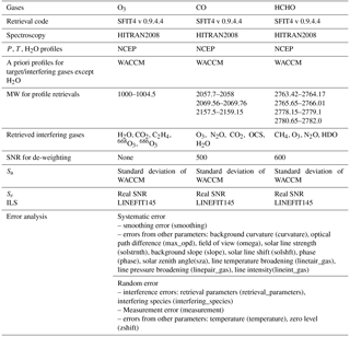
We assume measurement noise covariance matrices Sε to be diagonal and set their diagonal elements to the inverse square of the signal-to-noise ratio (SNR) of the fitted spectra and the non-diagonal elements of Sε to zero. For all gases, the diagonal elements of a priori profile covariance matrices Sa are set to the standard deviation of a dedicated WACCM run from 1980 to 2020, and its non-diagonal elements are set to zero.
We regularly used a low-pressure HBr cell to monitor the instrument line shape (ILS) and included the measured ILS in the retrieval (Hase, 2012; Sun et al., 2018).
3.2 Profile information in the FTS retrievals
The sensitive range for CO and HCHO is mainly tropospheric, and for O3 it is both tropospheric and stratospheric (Fig. S2). The typical degrees of freedom (DOFS) over the total atmosphere obtained at Hefei for each gas are included in Table 2: they are about 4.8, 3.5, and 1.2 for O3, CO, and HCHO, respectively. In order to separate independent partial column amounts in the retrieved profiles, we have chosen the altitude limit for each independent layer such that the DOFS in each associated partial column is not less than 1.0. The retrieved profiles of O3, CO, and HCHO can be divided into four, three, and one independent layers, respectively (Fig. S3). The troposphere is well resolved by O3, CO, and HCHO, where CO exhibits the best vertical resolution with more than two independent layers in the troposphere.
Table 2Typical degrees of freedom for signal (DOFs) and sensitive range of the retrieved O3, CO, and HCHO profiles at Hefei site.
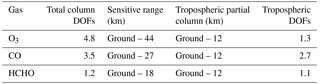
In this study, we have chosen the same upper limit (12 km) for the tropospheric columns for all gases (Table 2), which is about 3 km lower than the mean value of the tropopause (∼15.1 km). In this way we ensured the accuracies for the tropospheric O3, CO, and HCHO retrievals and minimized the influence of transport from the stratosphere, i.e., the so-called STE process (stratosphere–troposphere exchange).
3.3 Error analysis
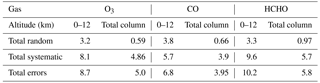
The results of the error analysis presented here are based on the average of all measurements that fulfill the screening scheme, which is used to minimize the impacts of significant weather events or instrument problems (Supplement Sect. S2). In the troposphere, the dominant systematic error for O3 and CO is the smoothing error, and for HCHO it is the line intensity error (Fig. S4). The dominant random error for O3 and HCHO is the measurement error, and for CO it is the zero baseline level error (Fig. S5). Taking all error items into account, the summarized errors in O3, CO, and HCHO for the 0–12 km tropospheric partial column and for the total column are listed in Table 3. The total errors in the tropospheric partial columns for O3, CO, and HCHO have been evaluated to be 8.7 %, 6.8 %, and 10.2 %, respectively.
Table 3Errors in % of the column amount of O3, CO, and HCHO for the 0–12 km tropospheric partial column and for the total column.
4.1 Tropospheric O3 seasonal variability
Figure 1a shows the tropospheric O3 column time series recorded by the FTS from 2014 to 2017, where we followed Gardiner's method and used a second-order Fourier series plus a linear component to determine the annual variability (Gardiner et al., 2008). The analysis did not indicate a significant secular trend of tropospheric O3 column probably because the time series is much shorter than those in Gardiner et al. (2008); the observed seasonal cycle of tropospheric O3 variations is well captured by the bootstrap resampling method (Gardiner et al., 2008). As commonly observed, high levels of tropospheric O3 occur in spring and summer (hereafter MAM/JJA). Low levels of tropospheric O3 occur in autumn and winter (hereafter SON/DJF). Day-to-day variations in MAM/JJA are generally larger than those in SON/DJF (Fig. 1b). At the same time, the tropospheric O3 column roughly increases over time in the first half of the year and reaches the maximum in June and then decreases during the second half of the year. Tropospheric O3 columns in June are 1.55×10¹⁸ molecules cm−2 (56 DU (Dobson units)) and in December are 1.05×10¹⁸ molecules cm−2 (39 DU). Tropospheric O3 columns in June were ∼50 % higher than those in December.
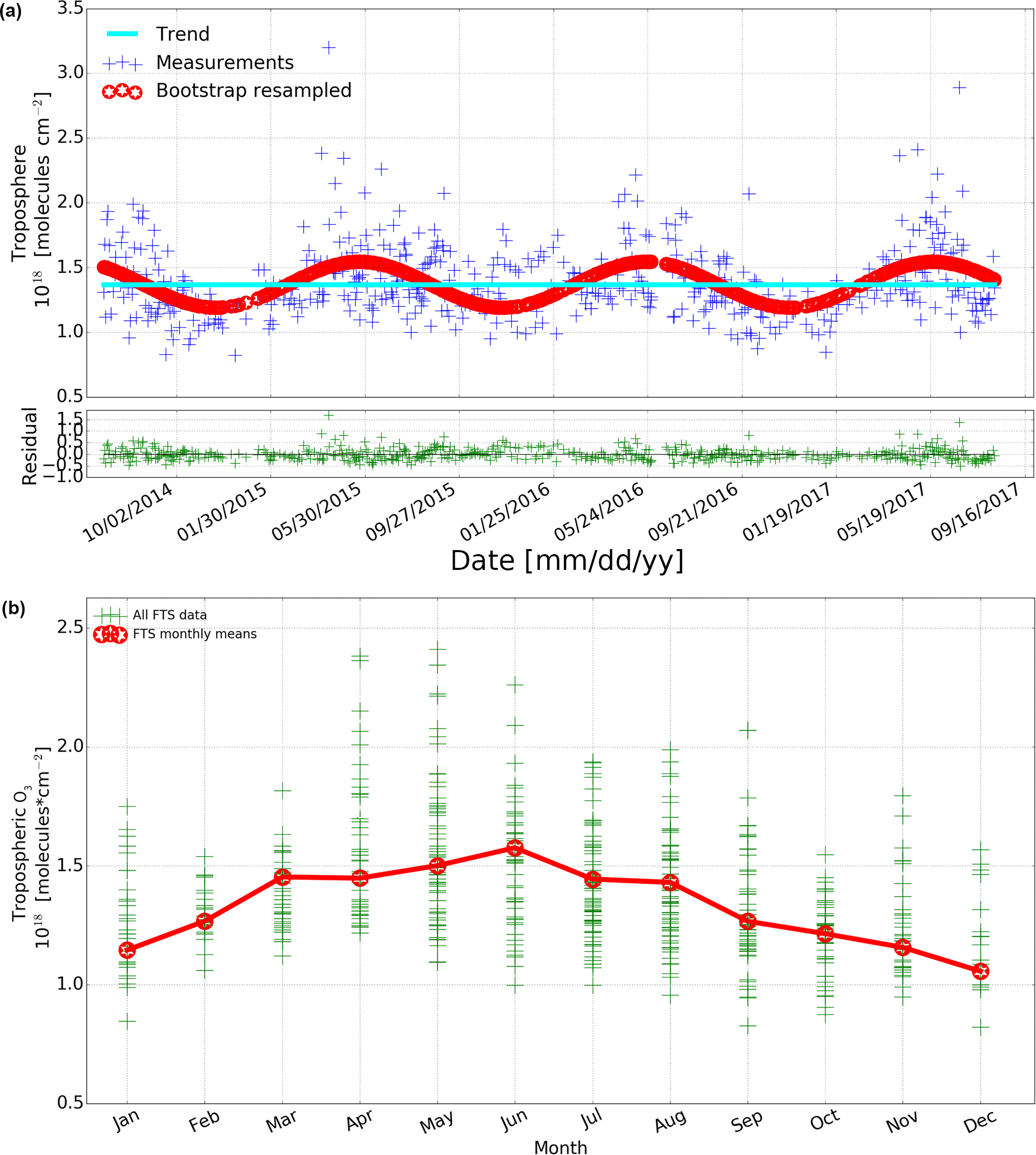
Figure 1(a) FTS measured and bootstrap resampled tropospheric O3 columns at Hefei site. The linear trend and the residual are also shown. Detailed description of the bootstrap method can be found in Gardiner et al. (2008). (b) Tropospheric O3 column monthly means derived from (a).
Vigouroux et al. (2015) studied the O3 trends and variabilities at eight NDACC FTS stations that have a long-term time series of O3 measurements, namely, Ny-Ålesund (79∘ N), Thule (77∘ N), Kiruna (68∘ N), Harestua (60∘ N), Jungfraujoch (47∘ N), Izaña (28∘ N), Wollongong (34∘ S), and Lauder (45∘ S). All these stations were located in non-polluted or relatively clean areas. The tropospheric columns at these stations are of the order of 0.7×10¹⁸ to 1.1×10¹⁸ molecules cm−2. The results showed a maximum tropospheric O3 column in spring at all these stations except at the high-altitude stations Jungfraujoch and Izaña, where it extended into early summer. This is because the STE process is most effective during late winter and spring (Vigouroux et al., 2015). In contrast, we observed a broader maximum at Hefei which extends over the MAM/JJA season, and the values are ∼35 % higher than those studied in Vigouroux et al. (2015). This is because the observed tropospheric O3 levels in MAM/JJA are more influenced by air masses originating from densely populated and industrialized areas (see Sect. 4.2), and the MAM/JJA meteorological conditions are more favorable to photochemical O3 production (see Sect. 5.1). The selection of tropospheric limits 3 km below the tropopause minimized but cannot avoid the influence of transport from the stratosphere; the STE process may also contribute to high level of tropospheric O3 column in spring.
4.2 Regional contribution to tropospheric O3 levels
In order to determine where the air masses came from and thus contributed to the observed tropospheric O3 levels, we have used the HYSPLIT (Hybrid Single-Particle Lagrangian Integrated Trajectory) model to calculate the three-dimensional kinematic back trajectories that coincide with the FTS measurements from 2014 to 2017 (Draxler et al., 2009). In the calculation, the GDAS (University of Alaska Fairbanks GDAS Archive) meteorological fields were used with a spatial resolution of , a time resolution of 6 h, and 22 vertical levels from the surface to 250 mbar. All daily back trajectories at 12:00 UTC, with a 24 h pathway arriving at Hefei site at 1500 m a.s.l., have been grouped into clusters and divided into MAM/JJA and SON/DJF seasons (Stunder, 1996). The results showed that air masses in Jiangsu and Anhui provinces in eastern China; Hebei and Shandong provinces in northern China; Shaanxi, Henan, and Shanxi provinces in northwestern China; and Hunan and Hubei provinces in central China contributed to the observed tropospheric O3 levels.
In the MAM/JJA season (Fig. 2a), 28.8 % of air masses are of eastern origin and arrived at Hefei through the southeast of Jiangsu Province and east of Anhui Province; 41.0 % are of southwestern origin and arrived at Hefei through the northeast of Hunan and Hubei provinces, and southwest of Anhui Province; 10.1 % are of northwestern origin and arrived at Hefei through the southeast of Shanxi and Henan provinces, and northwest of Anhui Province; 10.1 % are of northern origin and arrived at Hefei through the south of Shandong Province and north of Anhui Province; 10.1 % are of local origin generated in the south of Anhui Province. As a result, air pollution from megacities such as Shanghai, Nanjing, Hangzhou, and Hefei in eastern China; Changsha and Wuhan in central-southern China; Zhenzhou and Taiyuan in northwest China; and Jinan in north China could contribute to the observed tropospheric O3 levels.
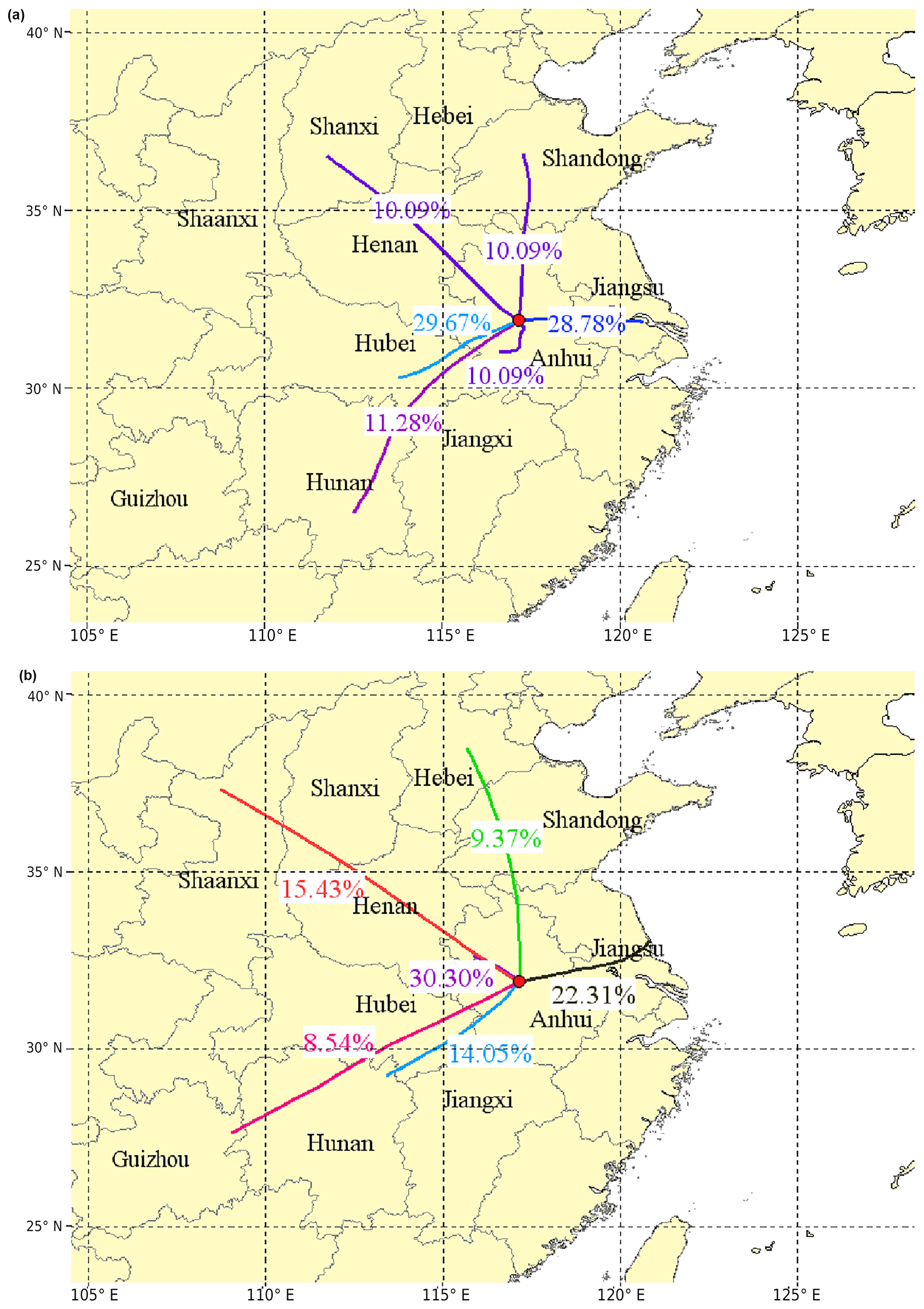
Figure 2One-day HYSPLIT back trajectory clusters arriving at Hefei at 1500 m a.s.l that are coincident with the FTS measurements from 2014 to 2017. (a) Spring and summer (MAM/JJA) and (b) Autumn and winter (SON/DJF) season. The base map was generated using the TrajStat 1.2.2 software (http://www.meteothinker.com, last access: 23 May 2018).
In the SON/DJF season, trajectories are generally longer and originated in the northwest of the MAM/JJA ones (Fig. 2b). The direction of air masses originating in the eastern sector shifts from the southeast to the northeast of Jiangsu Province, and that of local air masses shifts from the south to the northwest of Anhui province. Trajectories of eastern-origin, western-origin, and northern-origin air masses in SON/DJF are 6.5 %, 13.1 %, and 0.7 % less frequent than the MAM/JJA ones, respectively. As a result, the air masses outside Anhui province have a 20.2 % smaller contribution to the observed tropospheric O3 levels in SON/DJF than in MAM/JJA. In contrast, trajectories of local-origin air masses in SON/DJF are 20.2 % more frequent than the MAM/JJA ones, indicating a more significant contribution of air masses in Anhui province in SON/DJF.
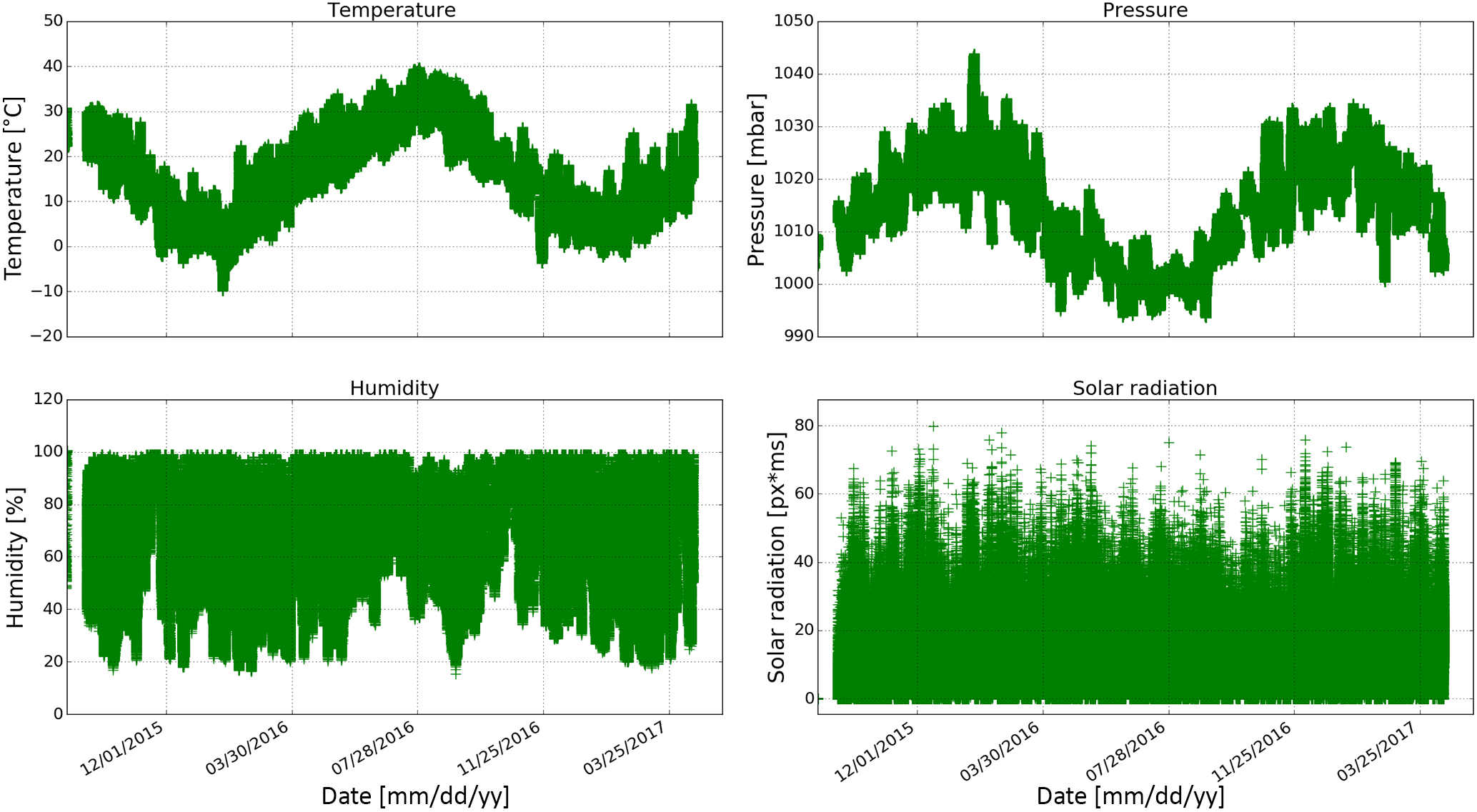
Figure 3Minutely averaged time series of temperature, pressure, humidity, and solar radiation recorded by the surface weather station.
The majority of the Chinese population lives in the eastern part of China, especially in the three most developed regions, the Jing–Jin–Ji (Beijing–Tianjin–Hebei), the Yangtze River Delta (YRD; including Shanghai–Jiangsu–Zhejiang–Anhui), and the Pearl River Delta (PRD; including Guangzhou, Shenzhen, and Hong Kong). These regions consistently have the highest emissions of anthropogenic precursors (Fig. S6), which have led to severe region-wide air pollution. This is particularly the case for the Hefei site, located in the central-western corner of the YRD, where the population in the southeastern area is typically denser than the northwestern area. Specifically, the southeast of Jiangsu province and the south of Anhui province are two of the most developed areas in YRD, and human activities therein are very intense. Therefore, when the air masses originated from these two areas, the O3 level is usually very high. Overall, compared with the SON/DJF season, the more southeastern air masses transportation in MAM/JJA indicated that the observed tropospheric O3 levels could be more influenced by the densely populated and industrialized areas, broadly accounting for the higher O3 level and variability in MAM/JJA.
5.1 Meteorological dependency
Photochemistry in polluted atmospheres, particularly the formation of O3, depends not only on pollutant emissions but also on meteorological conditions (Lei et al., 2008; Wang et al., 2017; Coates et al., 2016). In order to investigate the meteorological dependency of the O3 production regime in the observed area, we analyzed the correlation of the tropospheric O3 with the coincident surface meteorological data. Figure 3 shows time series of temperature, pressure, humidity, and solar radiation recorded by the surface weather station. The seasonal dependencies of all these coincident meteorological elements show no clear dependencies except for the temperature and pressure, which show clear reverse seasonal cycles. Generally, the temperatures are higher and the pressures are lower in MAM/JJA than those in SON/DJF. The correlation plots between the FTS tropospheric O3 column and each meteorological element are shown in Fig. 4. The tropospheric O3 column shows positive correlations with solar radiation, temperature, and humidity, and negative correlations with pressure.
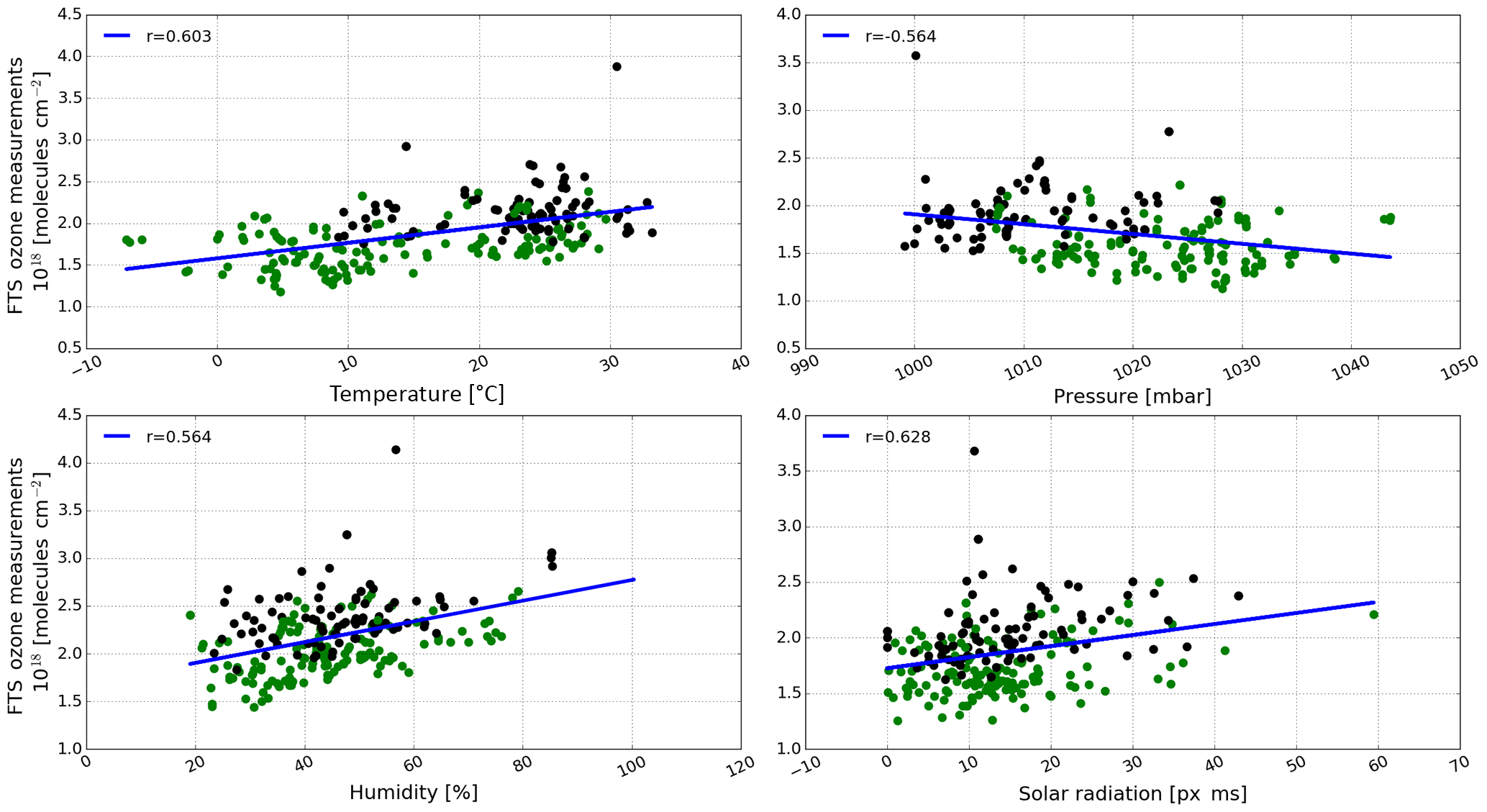
Figure 4Correlation plot between the FTS tropospheric O3 column and the coincident surface meteorological data. Black dots are data pairs within the MAM/JJA season and green dots are data pairs within the SON/DJF season.
High temperature and strong sunlight primarily affects O3 production in Hefei in two ways: by speeding up the rates of many chemical reactions and by increasing emissions of VOCs from biogenic sources (BVOCs) (Sillman and Samson, 1995b). While emissions of anthropogenic VOCs (AVOCs) are generally not dependent on temperature, evaporative emissions of some AVOCs do increase with temperature (Rubin et al., 2006; Coates et al., 2016). Elevated O3 concentration generally occurs on days with wet conditions and low pressure in Hefei, probably because these conditions favor the accumulation of O3 and its precursors. Overall, MAM/JJA meteorological conditions are more favorable to O3 production (higher sun intensity, higher temperature, wetter condition, and lower pressure) than SON/DJF, which supports the fact that tropospheric O3 in MAM/JJA is larger than that in SON/DJF.
5.2 PO3 relative to CO, HCHO, and NO2 changes
In order to determine the relationship between tropospheric O3 production and its precursors, the chemical sensitivity of PO3 relative to tropospheric CO, HCHO, and NO2 changes was investigated. Figure 5 shows time series of tropospheric CO, HCHO, and NO2 columns that are coincident with O3 counterparts. The tropospheric NO2 was deduced from the OMI product selected within the ±0.7∘ latitude/longitude rectangular area around the Hefei site. The retrieval uncertainty for the tropospheric column is less than 30 % (https://disc.gsfc.nasa.gov/datasets/OMNO2_V003/ last access: 23 May 2018). Tropospheric HCHO and NO2 show clear reverse seasonal cycles. Generally, tropospheric HCHO is higher and tropospheric NO2 is lower in MAM/JJA than in SON/DJF. Pronounced tropospheric CO was observed, but the seasonal cycle is not evident, probably because CO emission is not constant over the season or season dependent.
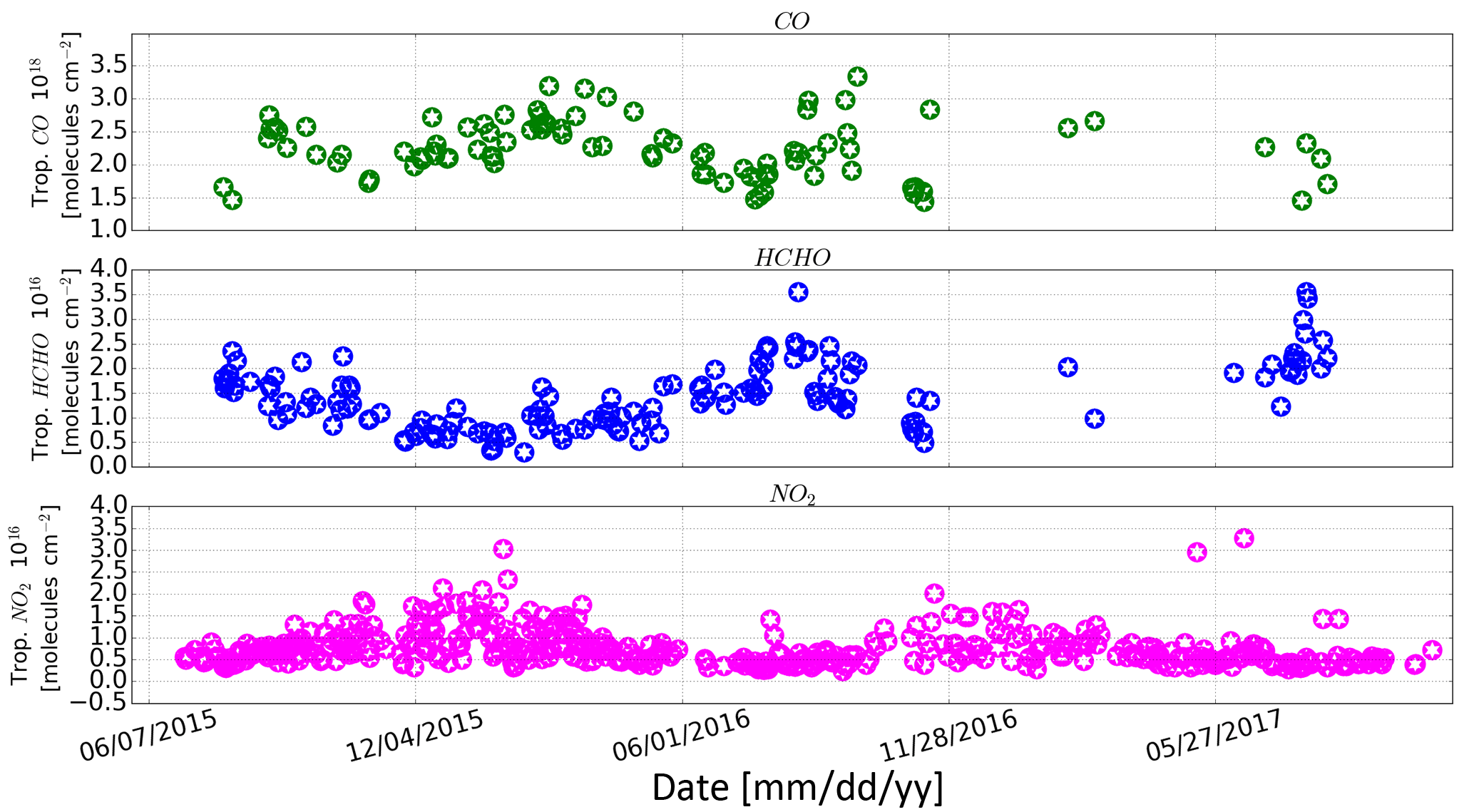
Figure 5Time series of tropospheric CO, HCHO, and NO2. Tropospheric CO and HCHO were derived from FTS observations, which is the same as tropospheric O3, and tropospheric NO2 is derived from OMI data.
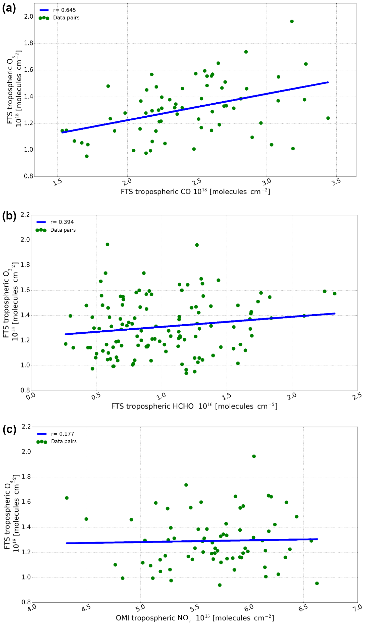
Figure 6Correlation plot between the FTS tropospheric O3 column and coincident tropospheric CO (a), HCHO (b), and NO2 (c) columns. The CO and HCHO data are retrieved from FTS observations, and the NO2 data were deduced from the OMI product.
Figure 6 shows the correlation plot between the FTS tropospheric O3 column and the coincident tropospheric CO, HCHO, and NO2 columns. The tropospheric O3 column shows positive correlations with tropospheric CO, HCHO, and NO2 columns. Generally, the higher the tropospheric CO concentration, the higher the tropospheric O3, and both VOCs and NOx reductions decrease O3 production. As an indicator of regional air pollution, the good correlation between O3 and CO (Fig. 6a) indicates that the enhancement of tropospheric O3 is highly associated with the photochemical reactions which occurred in polluted conditions rather than due to the STE process. The relatively weaker overall correlations of O3 with HCHO (Fig. 6b) and NO2 (Fig. 6c) are partly explained by different lifetimes of these gases, i.e., several hours to 1 day in summer for NO2 and HCHO and several days to weeks for O3. So older O3-enhanced air masses easily loose traces of NO2 or HCHO. Since the sensitivity of PO3 to VOCs and NOx is different under different limitation regimes, the relatively flat overall slopes indicate that the O3 pollution in Hefei can be fully attributed neither to NOx pollution nor to VOC pollution.
5.3 O3–NOx–VOC sensitivities
5.3.1 Transition/ambiguous range estimation
Referring to previous studies, the chemical sensitivity of PO3 in Hefei was investigated using the column HCHO∕NO2 ratio (Martin et al., 2004; Duncan et al., 2010; Witte et al., 2011; Choi et al., 2012; Jin and Holloway, 2015; Mahajan et al., 2015; Schroeder et al., 2017; Jin et al., 2017). The methods have been adapted to the particular conditions in Hefei. In particular the findings of Schroeder et al. (2017) have been taken into account.
Since the measurement tools for O3 and HCHO, the pollution characteristic, and the meteorological condition in this study were not the same as those of previous studies, the transition thresholds estimated in previous studies were not applied here (Martin et al., 2004a; Duncan et al., 2010; Witte et al., 2011; Choi et al., 2012; Jin and Holloway, 2015; Mahajan et al., 2015; Schroeder et al., 2017; Jin et al., 2017). In order to determine transition thresholds applicable in Hefei, China, we iteratively altered the column HCHO∕NO2 ratio threshold and judged whether the sensitivities of tropospheric O3 to HCHO or NO2 changed abruptly. For example, in order to estimate the VOC-limited threshold, we first fitted tropospheric O3 to HCHO that lies within column HCHO∕NO2 ratios <2 (an empirical starting point) to obtain the corresponding slope and then we decreased the threshold by 0.1 (an empirical step size) and repeated the fit, i.e., only fitted the data pairs with column HCHO∕NO2 ratios <1.9. This was done iteratively. Finally, we sorted out the transition ratio which shows an abrupt change in slope, and regarded this as the VOC-limited threshold. Similarly, the NOx-limited threshold was determined by iteratively increasing the column HCHO∕NO2 ratio threshold until the sensitivity of tropospheric O3 to NO2 changed abruptly.
The transition threshold estimation with this scheme exploits the fact that O3 production is more sensitive to VOCs if it is VOC-limited and is more sensitive to NOx if it is NOx limited, and there exists a transition point near the threshold (Martin et al., 2004a). Su et al. (2017) used this scheme to investigate the O3–NOx–VOC sensitivities during the 2016 G20 conference in Hangzhou, China, and argued that this diagnosis of PO3 could reflect the overall O3 production conditions.
5.3.2 PO3 limitations in Hefei
Through the above empirical iterative calculation, we observed a VOC-limited regime with column HCHO∕NO2 ratios <1.3, an NOx-limited regime with column HCHO∕NO2 ratios >2.8, and a mixed VOC–NOx-limited regime with column HCHO∕NO2 ratios between 1.3 and 2.8. Column measurements sample a larger portion of the atmosphere, and thus their spatial coverage is larger than in situ measurements. So the photochemical scene disclosed by column measurements is larger than the in situ measurement. Specifically, this study reflects the mean photochemical condition of the troposphere.
Table 4Chemical sensitivities of PO3 for the selected 106 days of observations that have coincident O3, HCHO, and NO2 counterparts.
Schroeder et al. (2017) argued that the column measurements from space have to be used with care because of the high uncertainty and the inhomogeneity of the satellite measurements. This has been mitigated in this study by the following.
The FTS measurements have a much smaller footprint than the satellite measurements. Also, we concentrate on measurements recorded during midday, when the mixing layer has largely been dissolved.
The measurements are more sensitive to the lower parts of the troposphere, which can be inferred from the normalized averaging kernels (AVKs). The reason is simply that the AVKs show the sensitivity to the column, but the column per altitude decreases with altitude.
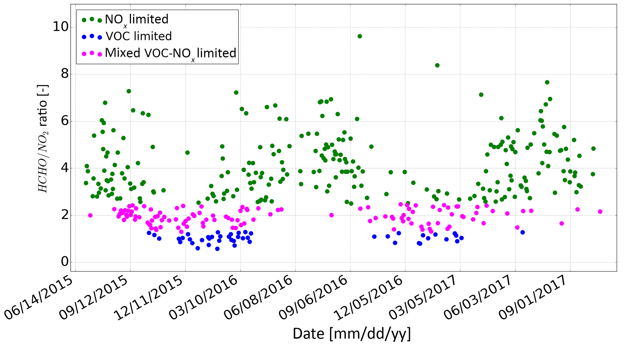
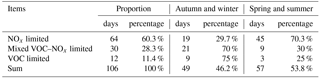
Figure 7 shows time series of column HCHO∕NO2 ratios which varied over a wide range from 1.0 to 9.0. The column HCHO∕NO2 ratios in summer are typically larger than those in winter, indicating that the PO3 is mainly NOx limited in summer and mainly VOC limited or mixed VOC–NOx limited in winter. Based on the calculated transition criteria, 106 days of observations that have coincident O3, HCHO, and NO2 counterparts in the reported period are classified, where 57 days (53.8 %) are in the MAM/JJA season and 49 days (46.2 %) are in the SON/DJF season. Table 4 lists the statistics for the 106 days of observations, which shows that NOx-limited, mixed VOC–NOx-limited, and VOC-limited PO3 accounts for 60.3 % (64 days), 28.3 % (30 days), and 11.4 % (12 days), respectively. The majority of NOx-limited (70.3 %) PO3 lies in the MAM/JJA season, while the majority of mixed VOC–NOx-limited (70 %) and VOC-limited (75 %) PO3 lies in the SON/DJF season. As a result, reductions in NOx and VOC could be more effective to mitigate O3 pollution in the MAM/JJA and SON/DJF seasons, respectively. Furthermore, considering most of PO3 is NOx limited or mixed VOC–NOx limited, reductions in NOx would reduce O3 pollution in eastern China.
We investigated the seasonal evolution and photochemical production regime of tropospheric O3 in eastern China from 2014 to 2017 by using tropospheric O3, CO, and HCHO columns derived from Fourier transform infrared spectrometry (FTS), the tropospheric NO2 column deduced from the Ozone Monitoring Instrument (OMI), the surface meteorological data, and a back trajectory cluster analysis technique. A pronounced seasonal cycle for tropospheric O3 is captured by the FTS, which roughly increases over time in the first half year and reaches the maximum in June, and then it decreases over time in the second half year. Tropospheric O3 columns in June are 1.55×10¹⁸ molecules cm−2 (56 DU (Dobson units)), and in December they are 1.05×10¹⁸ molecules cm−2 (39 DU). Tropospheric O3 columns in June were ∼50 % higher than those in December. A broad maximum within both spring and summer (MAM/JJA) is observed, and the day-to-day variations in MAM/JJA are generally larger than those in autumn and winter (SON/DJF). This differs from tropospheric O3 measurements in Vigouroux et al. (2015). However, Vigouroux et al. (2015) used measurements at relatively clean sites. Back trajectory analysis showed that air pollution in Jiangsu and Anhui provinces in eastern China; Hebei and Shandong provinces in northern China; Shaanxi, Henan, and Shanxi provinces in northwest China; and Hunan and Hubei provinces in central China contributed to the observed tropospheric O3 levels. Compared with the SON/DJF season, the observed tropospheric O3 levels in MAM/JJA are more influenced by the transport of air masses from densely populated and industrialized areas, and the high O3 level and variability in MAM/JJA is determined by the photochemical O3 production. The tropospheric-column HCHO∕NO2 ratio is used as a proxy to investigate the chemical sensitivity of the O3 production rate (PO3). The results show that PO3 is mainly nitrogen oxide (NOx) limited in MAM/JJA, while it is mainly VOC or mixed VOC–NOx limited in SON/DJF. Reductions in NOx and VOC could be more effective to mitigate O3 pollution in the MAM/JJA and SON/DJF seasons, respectively. Considering most of PO3 is NOx limited or mixed VOC–NOx limited, reductions in NOx would reduce O3 pollution in eastern China.
The SFIT4 software can be found via https://www2.acom.ucar.edu/irwg/links (last access: 23 May 2018). The data used in this paper are available on request.
The supplement related to this article is available online at: https://doi.org/10.5194/acp-18-14569-2018-supplement.
The first two authors contributed equally to this work. YS and CL prepared the paper with inputs from all coauthors. MP, CV, JN, NJ, and MDM designed the retrieval and optimized the content. QH and WS conceived ozone production regime study. WZ provided the OMI NO2 product. WW, CS, YT, XX, MZ, and JL carried out the experiments and performed back trajectory cluster analysis.
The authors declare that they have no conflict of interest.
This article is part of the special issue “Quadrennial Ozone Symposium 2016 – Status and trends of atmospheric ozone (ACP/AMT inter-journal SI)”. It is a result of the Quadrennial Ozone Symposium 2016, Edinburgh, United Kingdom, 4–9 September 2016.
This work is jointly supported by the National High Technology Research and
Development Program of China (no. 2016YFC0200800, no.2018YFC0213104, no.
2017YFC0210002, no. 2016YFC0203302), the National Science Foundation of
China (no. 41605018, no.41877309, no. 41405134, no.41775025, no. 41575021,
no. 51778596, no. 91544212, no. 41722501, no. 51778596), the Anhui Province
Natural Science Foundation of China (no. 1608085MD79), the Outstanding Youth
Science Foundation (no. 41722501), and the German Federal Ministry of
Education and Research (BMBF) (grant no. 01LG1214A). The processing and post-processing environments for SFIT4 are provided by the National Center for
Atmospheric Research (NCAR), Boulder, Colorado, USA. The NDACC networks are
acknowledged for supplying the SFIT software and advice. The HCHO
micro-windows were obtained at BIRA-IASB during the ESA PRODEX project TROVA
(2016–2018) funded by the Belgian Science Policy Office. The LINEFIT code is
provided by Frank Hase, Karlsruhe Institute of Technology (KIT), Institute
for Meteorology and Climate Research (IMK-ASF), Germany. The authors
acknowledge the NOAA Air Resources Laboratory (ARL) for making the HYSPLIT
transport and dispersion model available on the Internet. The authors would
also like to thank Jason R. Schroeder and three anonymous referees for
useful comments that improved the quality of this
paper.
Edited by: Stefan Reis
Reviewed by: five anonymous referees
Albrecht, T., Notholt, J., Wolke, R., Solberg, S., Dye, C., and Malberg, H.: Variations of CH2O and C2H2 determined from ground based FTIR measurements and comparison with model results, Adv. Space Res., 29, 1713–1718, https://doi.org/10.1016/S0273-1177(02)00120-5, 2002.
Boersma, K. F., Jacob, D. J., Trainic, M., Rudich, Y., DeSmedt, I., Dirksen, R., and Eskes, H. J.: Validation of urban NO2 concentrations and their diurnal and seasonal variations observed from the SCIAMACHY and OMI sensors using in situ surface measurements in Israeli cities, Atmos. Chem. Phys., 9, 3867–3879, https://doi.org/10.5194/acp-9-3867-2009, 2009.
Choi, Y., Kim, H., Tong, D., and Lee, P.: Summertime weekly cycles of observed and modeled NOx and O3 concentrations as a function of satellite-derived ozone production sensitivity and land use types over the Continental United States, Atmos. Chem. Phys., 12, 6291–6307, https://doi.org/10.5194/acp-12-6291-2012, 2012.
Coates, J., Mar, K. A., Ojha, N., and Butler, T. M.: The influence of temperature on ozone production under varying NOx conditions – a modelling study, Atmos. Chem. Phys., 16, 11601–11615, https://doi.org/10.5194/acp-16-11601-2016, 2016.
Duncan, B. N., Yoshida, Y., Olson, J. R., Sillman, S., Martin, R. V., Lamsal, L., Hu, Y., Pickering, K. E., Retscher, C., Allen, D. J., and Crawford, J. H.: Application of OMI observations to a space-based indicator of NOx and VOC controls on surface ozone formation, Atmos. Environ., 44, 2213–2223, https://doi.org/10.1016/j.atmosenv.2010.03.010, 2010.
Draxler, R. R., Stunder, B., Rolph, G., and Taylor, A.: HYSPLIT_4 User's Guide, via NOAA ARL website, NOAA Air Resources Laboratory, Silver Spring, MD, December 1997, revised January 2009, available at: http://www.arl.noaa.gov/documents/reports/hysplit user guide.pdf (last access: 19 May 2017), 2009.
Edwards, P. M., Young, C. J., Aikin, K., deGouw, J., Dubé, W. P., Geiger, F., Gilman, J., Helmig, D., Holloway, J. S., Kercher, J., Lerner, B., Martin, R., McLaren, R., Parrish, D. D., Peischl, J., Roberts, J. M., Ryerson, T. B., Thornton, J., Warneke, C., Williams, E. J., and Brown, S. S.: Ozone photochemistry in an oil and natural gas extraction region during winter: simulations of a snow-free season in the Uintah Basin, Utah, Atmos. Chem. Phys., 13, 8955–8971, https://doi.org/10.5194/acp-13-8955-2013, 2013.
Franco, B., Hendrick, F., Van Roozendael, M., Müller, J.-F., Stavrakou, T., Marais, E. A., Bovy, B., Bader, W., Fayt, C., Hermans, C., Lejeune, B., Pinardi, G., Servais, C., and Mahieu, E.: Retrievals of formaldehyde from ground-based FTIR and MAX-DOAS observations at the Jungfraujoch station and comparisons with GEOS-Chem and IMAGES model simulations, Atmos. Meas. Tech., 8, 1733–1756, https://doi.org/10.5194/amt-8-1733-2015, 2015.
Gardiner, T., Forbes, A., de Mazière, M., Vigouroux, C., Mahieu, E., Demoulin, P., Velazco, V., Notholt, J., Blumenstock, T., Hase, F., Kramer, I., Sussmann, R., Stremme, W., Mellqvist, J., Strandberg, A., Ellingsen, K., and Gauss, M.: Trend analysis of greenhouse gases over Europe measured by a network of ground-based remote FTIR instruments, Atmos. Chem. Phys., 8, 6719–6727, https://doi.org/10.5194/acp-8-6719-2008, 2008.
Hase, F.: Improved instrumental line shape monitoring for the ground-based, high-resolution FTIR spectrometers of the Network for the Detection of Atmospheric Composition Change, Atmos. Meas. Tech., 5, 603–610, https://doi.org/10.5194/amt-5-603-2012, 2012.
Jin, X. and Holloway, T.: Spatial and temporal variability of ozone sensitivity over China observed from the Ozone Monitoring Instrument, J. Geophys. Res.-Atmos., 120, 7229–7246, https://doi.org/10.1002/2015JD023250, 2015.
Jin, X. M., Fiore, A. M., Murray, L. T., Valin, L. C., Lamsal, L. N., and Duncan, B.: Evaluating a Space-Based Indicator of Surface Ozone-NOx-VOC Sensitivity Over Midlatitude Source Regions and Application to Decadal Trends, J. Geophys. Res.-Atmos., 122, 10231–10253, 2017.
Jones, N. B., Riedel, K., Allan, W., Wood, S., Palmer, P. I., Chance, K., and Notholt, J.: Long-term tropospheric formaldehyde concentrations deduced from ground-based fourier transform solar infrared measurements, Atmos. Chem. Phys., 9, 7131–7142, https://doi.org/10.5194/acp-9-7131-2009, 2009.
Kalnay, E., Kanamitsu, M., and Kistler, R.: The NCEP/NCAR 40-year reanalysis project, B. Am. Meteorol. Soc., 77, 437–472, 1996.
Kleinman, L., Daum, P., Lee, Y. N., Nunnermacker, L., Springston, S., Weinstein-Lloyd, J., Rudolph, J.: A comparative study of ozone production in five U.S. metropolitan areas, J. Geophys. Res.-Atmos, 110, D02301, https://doi.org/10.1029/2004JD005096, 2005.
Lei, W., Zavala, M., de Foy, B., Volkamer, R., and Molina, L. T.: Characterizing ozone production and response under different meteorological conditions in Mexico City, Atmos. Chem. Phys., 8, 7571–7581, https://doi.org/10.5194/acp-8-7571-2008, 2008.
Martin, R., Fiore, A., Van Donkelaar, A.: Space-based diagnosis of surface ozone sensitivity to anthropogenic emissions, Geophys. Res. Lett., 31, L06120, https://doi.org/10.1029/2004GL019416, 2004a.
Martin, R., Parrish, D., Ryerson, T., Nicks, D., Chance, K., Kurosu, T., Jacob, D., Sturges, E., Fried, A., and Wert, B.: Evaluation of GOME satellite measurements of tropospheric NO2 and HCHO using regional data from aircraft campaigns in the southeastern United States, J. Geophys. Res., 109, D24307, https://doi.org/10.1029/2004JD004869, 2004b.
Mahajan, A. S., De Smedt, I., Biswas, M. S., Ghude, S., Fadnavis, S., Roy, C., and van Roozendael, M.: Inter-annual variations in satellite observations of nitrogen dioxide and formaldehyde over India, Atmos. Environ., 116, 194–201, https://doi.org/10.1016/j.atmosenv.2015.06.004, 2015.
Millet, D. B., Jacob, D. J., Boersma, K. F., Fu, T.-M., Kurosu, T. P., Chance, K., Heald, C. L., and Guenther, A.: Spatial distribution of isoprene emissions from North America derived from formaldehyde column measurements by the OMI satellite sensor, J. Geophys. Res., 113, D02307, https://doi.org/10.1029/2007JD008950, 2008.
Oltmans, S. J., Lefohn, A. S., Harris, J. M., Galbally, I., Scheel, H. E., Bodeker, G., Brunke, E., Claude, H., Tarasick, D., Johnson, B. J., Simmonds, P., Shadwick, D., Anlauf, K., Hayden, K., Schmidlin, F., Fujimoto, T., Akagi, K., Meyer, C., Nichol, S., Davies, J., Redondas, A., and Cuevas, E.: Long-term changes in tropospheric ozone, Atmos. Environ., 40, 3156–3173, https://doi.org/10.1016/j.atmosenv.2006.01.029, 2006,
Rothman, L. S., Gordon, I. E., Barbe, A., Benner, D. C., Bernath, P. F., Birk, M., Boudon, V., Brown, L. R., Campargue, A., Champion, J.-P., Chance, K., Coudert, L. H., Danaj, V., Devi, V. M., Fally, S., Flaud, J.-M., Gamache, R. R., Goldmanm, A., Jacquemart, D., Kleiner, I., Lacome, N., Lafferty, W. J., Mandin, J.-Y., Massie, S. T., Mikhailenko, S. N., Miller, C. E., Moazzen-Ahmadi, N., Naumenko, O. V., Nikitin, A. V., Orphal, J., Perevalov, V. I., Perrin, A., Predoi-Cross, A., Rinsland, C. P., Rotger, M., Šime. cková, M., Smith, M. A. H., Sung, K., Tashkun, S. A., Tennyson, J., Toth, R. A., Vandaele, A. C., and Vander Auwera, J.: The Hitran 2008 molecular spectroscopic database, J. Quant. Spectrosc. Ra., 110, 533–572, 2009.
Rubin, J. I., Kean, A. J., Harley, R. A., Millet, D. B., and Goldstein, A. H.: Temperature dependence of volatile organic compound evaporative emissions from motor vehicles, J. Geophys. Res.-Atmos., 111, d03305, https://doi.org/10.1029/2005JD006458, 2006.
Schroeder, J. R., Crawford, J. H., Fried, A., Walega, J., Weinheimer, A., Wisthaler, A., Wisthaler, A., Muller, M., Mikoviny, T., Chen, G., Shook, M., Blake, D., and Tonesen, G. S.: New insights into the column CH2O∕NO2 ratio as an indicator of near-surface ozone sensitivity, J. Geophys. Res. Atmos., 122, 8885–8907, https://doi.org/10.1002/2017JD026781, 2017.
Sillman, S.: The use of NOy, H2O2, and HNO3 as indicators for ozone-NOx hydrocarbon sensitivity in urban locations, J. Geophys. Res., 100, 14175–14188, 1995a.
Sillman, S. and Samson, P. J.: Impact of temperature on oxidant photochemistry in urban, polluted rural and remote environments, J. Geophys. Res.-Atmos., 100, 11497–11508, 1995b.
Streets, D. G., Canty, T., Carmichael, G. R., de Foy, B., Dickerson, R. R., Duncan, B. N., Edwards, D. P., Haynes, J. A., Henze, D. K., Houyoux, M. R., Jacob, D. J., Krotkov, N. A., Lamsal, L. N., Liu, Y., Lu, Z., Martin, R. V., Pfister, G. G., Pinder, R. W., Salawitch, R. J., and Wecht, K. J.: Emissions estimation from satellite retrievals: A review of current capability, Atmos. Environ., 77, 1011–1042, https://doi.org/10.1016/j.atmosenv.2013.05.051, 2013.
Stunder, B.: An assessment of the Quality of Forecast Trajectories, J. Appl. Meteorol., 35, 1319–1331, 1996.
Su, W., Liu, C., Hu, Q., Fan, G., Xie Z., Huang, X., Zhang, T., Chen, Z., Dong, Y., Ji, X., Liu, H., Wang, Z., and Liu, J.: Characterization of ozone in the lower troposphere during the 2016 G20 conference in Hangzhou, Sci. Rep.-UK, 7, 17368, https://doi.org/10.1038/s41598-017-17646-x, 2017.
Sun, Y., Palm, M., Liu, C., Hase, F., Griffith, D., Weinzierl, C., Petri, C., Wang, W., and Notholt, J.: The influence of instrumental line shape degradation on NDACC gas retrievals: total column and profile, Atmos. Meas. Tech., 11, 2879–2896, https://doi.org/10.5194/amt-11-2879-2018, 2018.
Tang, G., Wang, Y., Li, X., Ji, D., Hsu, S., and Gao, X.: Spatial-temporal variations in surface ozone in Northern China as observed during 2009–2010 and possible implications for future air quality control strategies, Atmos. Chem. Phys., 12, 2757–2776, https://doi.org/10.5194/acp-12-2757-2012, 2012.
Tian, Y., Sun, Y. W., Liu, C., Wang, W., Shan, C. G., Xu, X. W., and Hu, Q. H.: Characterisation of methane variability and trends from near-infrared solar spectra over Hefei, China, Atmos. Environ., 173, 1352–2310, https://doi.org/10.1016/j.atmosenv.2017.11.001, 2018.
Tonnesen, G. S. and Dennis, R. L.: Analysis of radical propagation efficiency to assess ozone sensitivity to hydrocarbons and NO2. Long-lived species as indicators of ozone concentration sensitivity, J. Geophys. Res., 105, 9227–9241, https://doi.org/10.1029/1999JD900372, 2000.
Viatte, C., Strong, K., Walker, K. A., and Drummond, J. R.: Five years of CO, HCN, C2H6, C2H2, CH3OH, HCOOH and H2CO total columns measured in the Canadian high Arctic, Atmos. Meas. Tech., 7, 1547–1570, https://doi.org/10.5194/amt-7-1547-2014, 2014.
Vigouroux, C., Hendrick, F., Stavrakou, T., Dils, B., De Smedt, I., Hermans, C., Merlaud, A., Scolas, F., Senten, C., Vanhaelewyn, G., Fally, S., Carleer, M., Metzger, J.-M., Müller, J.-F., Van Roozendael, M., and De Mazière, M.: Ground-based FTIR and MAX-DOAS observations of formaldehyde at Réunion Island and comparisons with satellite and model data, Atmos. Chem. Phys., 9, 9523–9544, https://doi.org/10.5194/acp-9-9523-2009, 2009.
Vigouroux, C., Blumenstock, T., Coffey, M., Errera, Q., García, O., Jones, N. B., Hannigan, J. W., Hase, F., Liley, B., Mahieu, E., Mellqvist, J., Notholt, J., Palm, M., Persson, G., Schneider, M., Servais, C., Smale, D., Thölix, L., and De Mazière, M.: Trends of ozone total columns and vertical distribution from FTIR observations at eight NDACC stations around the globe, Atmos. Chem. Phys., 15, 2915–2933, https://doi.org/10.5194/acp-15-2915-2015, 2015.
Vigouroux, C., Bauer Aquino, C. A., Bauwens, M., Becker, C., Blumenstock, T., De Mazière, M., García, O., Grutter, M., Guarin, C., Hannigan, J., Hase, F., Jones, N., Kivi, R., Koshelev, D., Langerock, B., Lutsch, E., Makarova, M., Metzger, J.-M., Müller, J.-F., Notholt, J., Ortega, I., Palm, M., Paton-Walsh, C., Poberovskii, A., Rettinger, M., Robinson, J., Smale, D., Stavrakou, T., Stremme, W., Strong, K., Sussmann, R., Té, Y., and Toon, G.: NDACC harmonized formaldehyde time series from 21 FTIR stations covering a wide range of column abundances, Atmos. Meas. Tech., 11, 5049–5073, https://doi.org/10.5194/amt-11-5049-2018, 2018.
Wang, T., Xue, L. K., Brimblecombe, P., Lam, Y. F., Li, L., and Zhang, L.: Ozone pollution in China: A review of concentrations, meteorological influences, chemical precursors, and effects, Sci. Total Environ., 575, 1582–1596, 2017.
Wang, W., Tian, Y., Liu, C., Sun, Y., Liu, W., Xie, P., Liu, J., Xu, J., Morino, I., Velazco, V. A., Griffith, D. W. T., Notholt, J., and Warneke, T.: Investigating the performance of a greenhouse gas observatory in Hefei, China, Atmos. Meas. Tech., 10, 2627–2643, https://doi.org/10.5194/amt-10-2627-2017, 2017.
Wennberg, P. O. and Dabdub, D.: Atmospheric chemistry. Rethinking ozone production, Science, 319, 1624-5 https://doi.org/10.1126/science.1155747, 2008.
Witte, J. C., Duncan, B. N., Douglass, A. R., Kurosu, T. P., Chance, K., and Retscher, C.: The unique OMI HCHO∕NO2 feature during the 2008 Beijing Olympics: Implications for ozone production sensitivity, Atmos. Environ., 45, 3103–3111, https://doi.org/10.1016/j.atmosenv.2011.03.015, 2011.
Xing, C., Liu, C., Wang, S., Chan, K. L., Gao, Y., Huang, X., Su, W., Zhang, C., Dong, Y., Fan, G., Zhang, T., Chen, Z., Hu, Q., Su, H., Xie, Z., and Liu, J.: Observations of the vertical distributions of summertime atmospheric pollutants and the corresponding ozone production in Shanghai, China, Atmos. Chem. Phys., 17, 14275–14289, https://doi.org/10.5194/acp-17-14275-2017, 2017.