2.1 The aerosol model

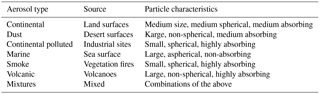
An aerosol model was developed to calculate the optical properties of pure aerosols which are generated by a single source (e.g. dust produced by the deserts, marine particles produces by the oceans). In this article, six classes of pure aerosol are considered: continental, continental polluted, dust, marine, smoke, and volcanic (Table 1). The aerosol model combines the Global Aerosol Data Set (Koepke et al., 1997) along with the T-matrix numerical method (Mishchenko et al., 1996; Waterman, 1971) to iteratively compute the intensive optical properties of each aerosol type. The chemical composition of each pure aerosol type was picked up from the OPAC (Optical Properties of Aerosols and Clouds) software package (Hess et al., 1998). The chemical composition of each aerosol type was varied in certain limits (the limits are detailed in Table 2 and refer to particle number density mixing ratios) in order to reproduce the large variety of particles present in the atmosphere. The synthetic database developed using the aerosol model is built for 350, 550, and 1000 nm sounding wavelengths. These wavelengths were selected from the 61 wavelengths (0.25–40 µm) of OPAC for which the microphysical characteristics of the aerosols are available from GADS. The selected wavelengths are then rescaled to the usual lidar wavelengths (i.e. 355, 532, and 1064 nm) using an Ångström exponent equal to 1. This was considered a valid assumption for all aerosol types, taking into account the small difference between the lidar and the model wavelengths. If required, the aerosol model can be extended to other wavelengths.

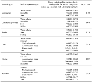
Each pure aerosol type is built as an internal mixture of basic components which do not interact physically or chemically, having different mixing ratios. The basic components are picked up from OPAC: water soluble, insoluble, soot, mineral (nucleation, accumulation, coarse), sulfates, and sea salt (accumulation, coarse). The GADS database is used for the microphysical properties of each component (Koepke et al., 1997). However, with the current values of the complex refractive index of soot in GADS, values greater than 1.2 for the Ångström exponent (550∕350 nm) cannot be achieved for smoke and continental-polluted types. Based on the findings of Schnaiter et al. (2003) and Henriksen et al. (2007), a typical value of 1.41 was considered for the real part of the refractive index, instead of 1.75 as it is currently in GADS.

In the aerosol model, particles were considered to be spheroids with different aspect ratios (i.e. the ratio of the polar to equatorial lengths) to simulate the aerosol anisotropy (Table 2). Dust and volcanic aerosols were considered oblate (i.e. aspect ratio <1). Also, the proportion of soot was increased to counterbalance for the low hematite (iron oxide) content, consistent with Dubovik et al. (2002) and Gasteiger et al. (2011b).

Starting from the microphysical properties (i.e. mode radius, width of the log-normal distribution, number density, density, and mass concentration) of each component, the microphysical properties of the pure aerosol were calculated by varying the critical component in certain limits (i.e. its number density mixing ratio), while the total mixture is normalized to 1 (Table 2). The mixing ratio of the aerosol components is given by

where NC represents the number of components, N_t is the total number of particles, N_j is the number of particles for component j, and the boundary condition is given by

For each wavelength selected in the aerosol model, the real and the imaginary parts of the complex refractive index were determined with the Lorentz–Lorentz model:

where m_p and m_j represent the complex refractive index for the particle and for the j components of the aerosol mixture. The aerosol radius (r_p) is calculated with the following equation

where $r_j^{\text{mod}}$ is the radius of the component j with respect to relative humidity (RH). The aerosol size distribution (n(r)) as a function of aerosol radius (r) assuming mono-modal log-normal distribution is given by

where ${\mathit{\sigma }}_p={\sum }_j{\mathit{\mu }}_j\cdot {\mathit{\sigma }}_j$ represents the width of the distribution for aerosols, and σ_j is the width of the distribution for component j (computed as the standard deviation of the log of the distribution with $r_j^{\text{mod}}$ mod radius).

Using the calculated microphysical properties with the T-matrix code (Mishchenko and Travis, 1994), the effective cross section for the particle scattering (C_sca) and extinction (C_ext) as well as the scattering matrix elements (phase functions) were obtained. These parameters are further used to determine (for a single particle) the aerosol optical parameters. The extinction coefficient (α) is determined from Eq. (6) and the backscatter coefficient (β) from Eq. (7), where F₁₁ is the first element of the scattering matrix (phase function).

The integration domain (R_min:R_max), for which the effective radius, the extinction coefficient, and scattering coefficient are calculated, covers medium-size particles with a radius between 0.1 and 5.0 µm that contribute to the scattering and extinction of light. The radius was not increased further due to computing time limitations and model design limitations (i.e. the code used for the calculation of the optical parameters for spheroids does not achieve the convergence for non-spherical particles). However, the latter limitation is not considered critical for the range of lidar wavelengths.

The single-scattering albedo ($\stackrel{\mathrm{‾}}{\mathit{\omega }}$) is yielded as the ratio of the scattering and extinction effective cross sections:

The lidar ratio (LR) is determined by the following relationship,

while the particle linear depolarization (δ) is calculated based on the elements of the scattering matrix,

The algorithm is iterated for each composition, wavelength, and RH value until the entire selected domain is covered. The domain represents the range in which the parameters are varied (e.g. the domain for the wavelength is [350, 500, 1000 nm]; the domain for RH is [50 %, 70 %, 80 %, 90 %]; the domain for the number density mixing ratios for each component of each pure aerosol type is listed in Table 2). The algorithm generates the properties and mixing ratio of each component, the optical and microphysical properties of the aerosol, for each wavelength, each RH value, and each composition.

Four classes of RH (i.e., 50 %, 70 %, 80 %, 90 %) are considered, out of the eight classes in OPAC. The high RH values (i.e. above 90 %) were excluded in order to avoid ambiguous results related to activation of the hygroscopic particles. Dry particles, those with 0 % RH, considered too rarely present in the ambient atmosphere. For a better representation of the particle growth, the OPAC RH classes were linearly interpolated with a 1 % step for pure types and 5 % for mixed types and linearly extrapolated down to 40 %. Thus, within a 40 %–90 % range the hygroscopic growth is considered linear for all pure aerosols included in the model.

Even while considering a certain variation of the aerosol composition and of RH, the simulated optical parameters are not covering the whole range of measured values. This is partly due to the limitations of the model itself and partly due to the various uncertainties associated with the measurements, either due to the instrument (e.g. biases, calibration) or due to the data treatment (e.g. algorithms applied in preprocessing to correct or average raw signals, algorithms used to calculate data products). Optical parameters calculated from lidar measurements are reported in the EARLINET database as the mean value (x_med) and associated uncertainty (absolute error, Δx). Optical parameters calculated from synthetic data do not carry this uncertainty; therefore a fixed relative error was considered, which was multiplied with the value to obtain the absolute error (uncertainty). For the actual retrieval of the aerosol type, any value between (x_med−uncertainty) and (x_med+uncertainty) was possible; therefore the algorithm was applied for all these values with a certain step (i.e. the finesse). The output is a “bundle” of possible aerosol types, with a dimension equal to the finesse. A compromise should be made between the finesse and computing time.

Based on the values reported in the literature (Ansmann et al., 2002; Freudenthaler et al., 2009), a large uncertainty is associated with the extinction coefficient derived with the Raman method, mainly due to noisy Raman lidar signals (i.e. the relative error reported in the lidar measurements is 30 %–150 % and the fixed relative error considered in the synthetic data is 50 %). Particle depolarization is very sensitive to the calibration, both for the raw signals of the two channels and for the backscattering. Thus, the values for particle depolarization also have a significant uncertainty (i.e. the relative error reported in the lidar measurements is 2 %–50 % and the fixed relative error considered in the synthetic data is 30 %). The backscatter coefficient calculated from the combination of Raman-elastic channels is less sensitive (i.e. the relative error reported in the lidar measurements is 10 %–50 % and the fixed relative error considered in the synthetic data is 20 %). Even in the case of HSRL, for which the extinction and the backscattering are independently calculated, the cross-talk between the Mie and the Rayleigh channels still introduces systematic errors, which are larger for the extinction than for the backscattering.

The relative errors considered here are 50 % for the extinction, 20 % for the backscattering and 30 % for the depolarization. Note that these values were assumed to be inclusive to mimic high-precision but also moderate-precision retrieved parameters. Although for the microphysical inversion the recommended maximum value for the uncertainty of the optical parameters is 20 % (Müller et al., 1999a, b), this is not critical for aerosol classification, as long as a relevant number of parameters is provided (e.g. measured lidar ratios and Ångström exponent are required).

Figure 1The generation chain of the synthetic data for the NATALI algorithm.

Download

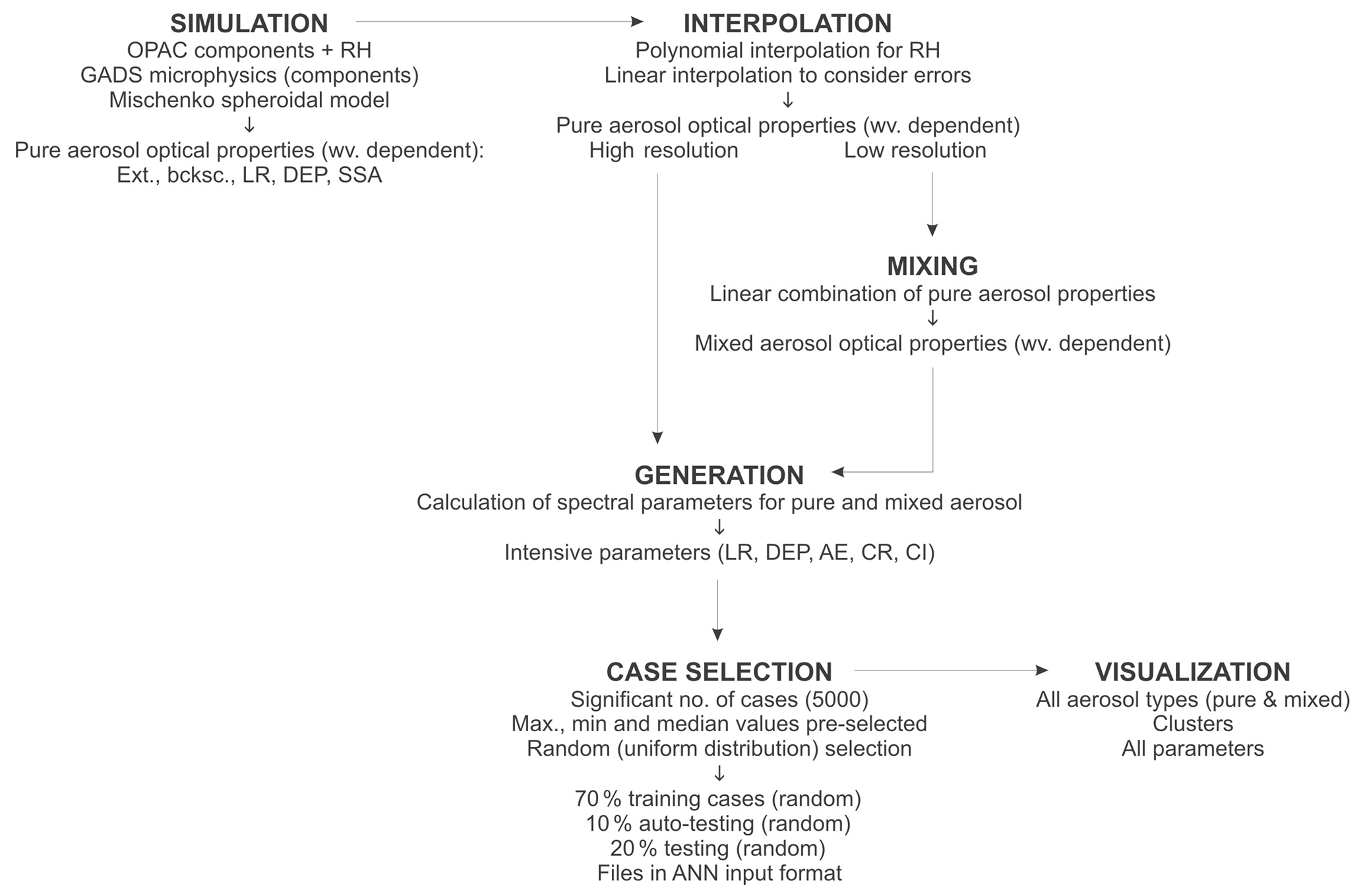
Table 4 shows the aerosol types considered in this study: six pure aerosols, seven mixtures of two pure aerosols, and two mixtures of three pure aerosols. The mixtures were obtained by linear combination of pure aerosol properties. The mixtures composed of only two pure types were considered not sufficient. For example, transcontinental transport involves at least three types of pure aerosols (e.g. transport from Africa to Europe can result in a mixture of continental, dust, and marine aerosols). Adding marine aerosols drastically changes the optical properties of the mixtures of two pure aerosols. Thus, mixtures of three aerosol types were considered, especially those containing marine types. From the total number of possible mixtures of two and three aerosols (i.e. 35 mixtures), only those that are most frequently observed and can still be distinguished were selected (i.e. 9 mixtures; see Table 4). This selection of mixtures was also a compromise between the time performance of the algorithm and the minimum number of output aerosol types considered significant in atmosphere.

The generated optical properties of pure aerosols and mixtures serve as a basis for the determination of the extinction Ångström exponent (κ_ext) and the backscatter Ångström exponent (κ_bsca), also referred to as a colour ratio, for each wavelength combination (Fig. 1). Thus, the Ångström exponent is given by the relationship

Similarly, the backscatter Ångström coefficient (colour index) can be determined using the equation

After the calculation of the spectral parameters for pure and mixed aerosols, the synthetic data are used as an input for the artificial neural networks.

2.2 The architecture artificial neural networks

The ANNs can be calibrated or “trained” for a specific purpose. Here, ANNs are trained to classify aerosols using solely the lidar intensive properties as input data, without any complementary information. The ANNs used here to classify aerosols were developed using NeuroSolutions a neural network development environment. Several ANNs architectures have been explored: Multilayer Perceptron (MLP), Jordan/Elman Network (JE), Generalized Feed Forward Network (GFF), Self-Organizing Feature Maps (SOFM), Recurrent Neural Network (RNN). Each ANN architecture contains several hidden layers and different learning rules. Each layer is composed of a vector of processing elements of identical parameters (e.g. TanhAxon, SigmoidAxon, LinearTanhAxon) with an associated learning rule and learning parameters.

No significant improvement in the classification of the aerosols has been achieved for different types of processing elements on the ANN structure. Thus, TanhAxon were subsequently used. The TanhAxon applies a bias and a hyperbolic tangent function (i.e. tanh) to each neuron in the layer and replaces a part of the tanh by a line with a slope β. The values of each neuron are forced to be in the interval −1 and 1. For TanhAxon the activation function is defined as

where $x_i^{\text{lin}}=\mathit{\beta }{x}_i$ and w_i is the bias vector.

Table 3Selected types of artificial neural networks and their structures.

Download Print Version | Download XLSX

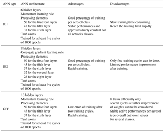
Table 4Correspondence between the aerosol types defined in the algorithm, as they can be retrieved by NATALI in high resolution and low resolution.

Download Print Version | Download XLSX

Supervised training has been used to train ANNs. Thus, sets of input and output parameters have been being successively presented to the networks for around 1000 epochs (i.e. one forward pass and one backward pass of all the training examples) per training cycle. Backpropagation is the most common form for training ANNs with more than one hidden layer. In the case of backpropagation, the weights on input elements are changed based on their previous value and a correction term. This training approach has been used also for the design of the NATALI ANN: the input data being continuously presented to the ANN and the output compared with the known aerosol type from synthetic database in order to adjust the weights until the desired result is achieved. The optimal values of weights and the minimum errors were taken into account for the testing process. The minimum classification errors were 75 % for more than 80 % of the measured data and 75 % for more than 90 % of the synthetic data.

Several learning rules have been tested: momentum, conjugate gradient descent, step, and Levenberg–Marquardt. The momentum learning rule is a simple and efficient approach in comparison with a standard gradient. It provides the gradient descent with some inertia, depending on the momentum parameter, which gives the smoothness of the gradient estimation. The momentum parameter is the same for all processing elements on a layer. The conjugate gradient has no parameters that need to be adjusted (e.g. learning rates, momentum parameter) and is faster and more accurate with respect to the standard backpropagation. The other two rules, the step rule – a type of standard gradient descent algorithm that allows the user to set a default step size for all weights within the activation component – and the Levenberg–Marquardt rule, which gives a numerical solution to the problem of minimizing a non-linear function, were found inadequate for aerosol-typing purpose. The step rule recognized all aerosol types after the first training cycle, but its active performance was low. The Levenberg–Marquardt algorithm was blocked after several epochs.

Figure 2Artificial neural network logical scheme for the NATALI algorithm.

Download

The cross-validation and test set methods have been used to stop the learning process and to assess the performances. Cross-validation monitors the error for a set of data and stops training when this error begins to increase. After a full process of training, in our case 5–10 training cycles, a testing set of data is presented to the ANN and the network output is compared with the known aerosol type from the synthetic database. In total 68 ANN structures have been explored, starting from the simplest (reduced number of hidden layers) to the most complex ones in order to compromise between the minimum possible time of training and testing, and avoiding saturation effects. Examples of six pure, seven double-component mixtures, and two triple-component mixtures obtained within the 68 explored ANN are presented in Table 4. For the selection of the ANNs, the synthetic database has been split randomly into data used to train the ANN (70 % of all synthetic data sets), data used to test ANN (20 % of all synthetic data sets), and data used for validation (10 % of all synthetic data sets). In the training process, data sets are presented to the ANN with the correct answer. The training is performed iteratively until the testing and validation classification errors are below 25 % (Fig. 2). A finer adjustment of the weighting coefficients is done during the testing process. The last 10 % of the data are presented to the ANN without the known result in order to validate the optimum training process and the capability of the network to classify new data inputs.

Three basic ANNs (adjusted to accommodate all data) have been chosen as appropriate to classify the multiwavelength lidar data in parallel, for both high- and low-resolution classification: the Jordan–Elman with 6 or 8 hidden layers, and the generalized feedforward with 10 hidden layers (Table 3). The selected types of ANNs classify the aerosols based on the response with higher confidence (i.e. the probability of having one of the aerosol types). The ANNs have been trained using 3500 samples for each aerosol type and successive training sessions until the best weights are reached (i.e. the classification process is ended, and the classification errors are low).

Figure 3Schematics of the NATALI algorithm for aerosol typing.

Download

2.3 The typing algorithm

Following the methodology described in Sect. 2.1 and taking into account the uncertainty threshold of each optical parameter, a bundle of inputs for each measured or simulated aerosol layer was generated. Answers with low confidence are filtered out (e.g. by using a threshold of minimum 0.7 confidence). The correct answer is selected based on a statistical approach considering two criteria: (a) which answer has a higher confidence; (b) which answer is more stable over the uncertainty range.

The input parameters for NATALI are typical data products from EARLINET database: backscatter coefficient (β) profiles at 1064, 532 and 355 nm, extinction coefficient (α) profiles at 532 and 355 nm, and, optionally, linear particle depolarization (δ) profile at 532 nm. The identification of aerosol types is not always possible due to its dependence on the physical content (i.e. with or without δ) and the quality of the optical data (i.e. calibration, uncertainty). For these reasons three classification schemes are used with different aerosol type resolutions (Table 4). First, when particle depolarization is available and all optical parameters are provided with a high-quality (uncertainty of the aerosol extinction coefficient ≤50 %, uncertainty of the aerosol backscatter coefficient ≤20 %, uncertainty of the particle linear depolarization ration ≤30 %), the typing is performed in high resolution (AH). This means that the mixtures can be resolved and the number of outputs is 14 (i.e. pure with minimum 90 %, mixtures of two, and mixtures of three pure aerosol types). Second, when particle depolarization is available and the optical parameters have a high uncertainty (uncertainty of the aerosol extinction coefficient >50 %, uncertainty of the aerosol backscatter coefficient >20 %, uncertainty of the particle linear depolarization ration >30 %), the typing is performed in low resolution (AL). In this case, the number of outputs is six (i.e. pure with maximum 30 % traces of other types). Third, when the particle depolarization is not available, the typing is performed in low resolution, again meaning that the mixtures cannot be resolved. In this case, the predominant aerosol type is retrieved for four outputs (pure with maximum 30 % traces of other types), whereby if only spectral parameters are provided, the volcanic type cannot be distinguished from dust nor continental pollution and are therefore excluded as output.

The three ANNs (Table 3) were developed for three classification schemes (Table 4) to increase the confidence of the aerosol typing. A voting procedure selects the most probable answer out of the three (possibly different) individual returns. The selection is made based on the confidence level of the ANN outputs and stability over the uncertainty range (i.e. the percentage of agreement for values between error limits).

2.4 The NATALI code

The Neural Network Aerosol Typing Algorithm based on LIdar data (NATALI) developed in the Python programming language is built on three modules: (a) an input module to prepare the inputs in the specific format of the ANNs, (b) a typing module to run the ANNs and decide on the most probable aerosol type and (c) an output module to save the results and logs. The input module reads the lidar files in EARLINET NetCDF format, checks for the availability of all required parameters (β1064, β532, β355, α532, α355, and optionally δ532 nm), identifies the layer geometrical boundaries and calculates within each layer the mean intensive optical parameters (i.e. Ångström exponent, colour indexes colour ratios, lidar ratios, particle linear depolarization ratio) and their associated uncertainty) (Fig. 3).

The layer boundaries are calculated by applying the gradient method on the 1064 nm backscatter coefficient profile (Belegante et al., 2014). The inflexion points of the second derivative of the profile data, computed with the Savitzky-Golay filter, give the top and the bottom of the layers. The window size of the cubic Savitzky–Golay filter, which is modified by the user, has a default value of 700 m. The filter was applied twice to obtain the second derivative. A signal-to-noise ratio filter is applied at this point, making sure the ratio is at least 5. The layer boundaries are moved towards the median height until the SNR criteria is met; if the criteria cannot be satisfied with a layer height greater than 300 m, the layer is discarded. A coarse or fine structure of the aerosol layers is revealed by a higher or lower value of the adjustable smoothing parameter (FINESSE). The layers with thicknesses of more than 300 m are considered, whereby the intensive optical properties and their uncertainties are computed for the middle of each layer in the range of at least 200 m thickness to exclude the margins likely affected by the smoothing

Several filters are applied to the data, and only layers which pass the following criteria are further considered for typing:

• availability of all necessary intensive optical parameters,

• values of the intensive optical parameters are between acceptable limits (Table 5),

• the relative error of each intensive optical parameter is lower than 50 %.

Table 5Acceptable limits for the layer average intensive optical parameters.

Download Print Version | Download XLSX

For each layer and for each intensive optical parameter, the input module generates an adjustable number N of values x with uncertainties (Δx) in the range x−Δx and x+Δx. Data are than scrambled considering that any combination has a similar probability to describe the reality. The cluster of possible combinations of intensive optical parameters is then converted into the ANN input format.

The typing module runs parallel to the ANNs for each data set representing a layer, and applies the voting procedure to identify the most probable aerosol type. In the case that the depolarization is available, the module runs in six parallel ANNs, three for high resolution (i.e. A1H, A2H, A3H) and three for low-resolution typing (i.e. A1L, A2L, A3L). The probable aerosol type is provided by the high-resolution ANNs, while the predominant type is provided by the low-resolution ANNs. As such, if typing in high resolution fails due the data quality, the user still has access to information in low resolution. If the depolarization is not available, the module runs three ANNs (i.e. B1L, B2L, B3L) in parallel and returns only the most probable predominant aerosol type (volcanic overlaps, in all existing parameters, completely with dust or continental-polluted type and cannot be retrieved in low resolution). The output module prepares and saves the files in two formats, csv and human-readable (telegrams) files, and writes a log. The csv files and the telegrams contain the identification of the data sets for which typing is performed and provide the following parameters:

• identification of the data sets for which the typing was performed;

• for each identified layer

  • the geometrical top and bottom,

  • the intensive optical parameters and associated uncertainties,

  • the aerosol type retrieved by each ANN, and the number of agreements,

  • the most probable type selected with the voting procedure (in low and high resolution separately if so),

  • the type of the ANN delivering the result (i.e. 1, 2, or 3),

  • comments generally referring to situations in which optical data did not pass the quality criteria or errors in the retrieval procedure.

Table 6Optical properties of aerosols from the synthetic data set and measurements.

Download XLSX

The NATALI code additional information (e.g. run time, run parameters, network error messages) is included in the telegrams. The software structure resembles the three module approach described earlier: an input module (nt_input.py), a typing module (nt_typing.py), and an output module (nt_output.py). The three modules are coordinated by the natali.py script, which contains the high-level algorithm and calls the required module routines/codes.

3.1 Comparison of the aerosol model with the literature

Synthetic aerosol optical properties, i.e. Ångström exponent (AE_{550_350}), colour ratios (CR_{550_350} and, CR_{1000_550)}), lidar ratios (LR₃₅₀ and LR₅₅₀), and linear particle depolarization ratio at 550 nm (DEP₅₅₀) generated by the developed aerosol model have been compared with the measured intensive parameters for the six classes of pure aerosol. The comparison with previous literature was only possible for pure types because the properties of mixed aerosols are computed based on a linear progression of the corresponding optical properties for two pure types. As shown in Table 6, the synthetic data are in general in very good agreement with the values reported in previous studies (i.e. the range of synthetic values is between the minimum and maximum values reported in the literature). Synthetic values lower than those observed are for continental-rural (AE_{550_350}), continental-polluted (CR_{1000_500}), and dust (CR_{1000_500}) types. Synthetic values greater than those from the literature are for continental-rural (LR₃₅₀) and volcanic (DEP₅₅₀) types. The reasons for these discrepancies are many. In some cases, values reported in the literature have high uncertainties because of natural variability, improper calibration, and retrieval. The aerosol model has also some limitations, e.g. due to spheroidal model and mono-modal log-normal distribution.

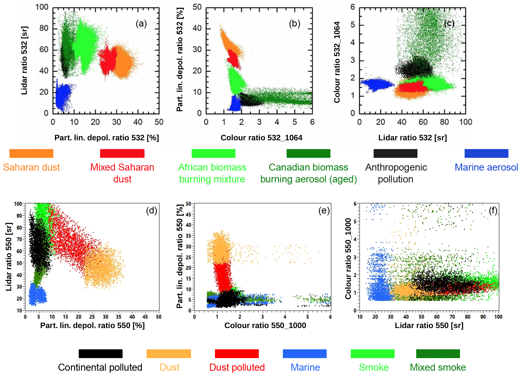
Figure 4Characteristic quantities of various atmospheric aerosol types form lidar measurements (a–c, adapted from Groß et al., 2013, their Fig. 5) and from synthetic measurements (d–f). (a, d) Lidar ratio versus linear particle depolarization. (b, e) Linear particle depolarization versus colour ratio. (c, f) Colour ratio versus lidar ratio.

Download

When comparing the aerosol model with the results from the previous studies, the changes in OPAC concerning the hygroscopic growth need to be considered (Zieger et al., 2013). These changes have not been implemented here, because when this study was conducted the new OPAC hygroscopicity was not available. However, the changes in OPAC are not expected to produce major changes in the aerosol model, considering the large uncertainties introduced to the model to simulate the observations.

In Fig. 4 comparisons between the synthetic data for pure aerosol obtained from the model and the measurements obtained by Groß et al. (2013) are provided. Based on the Airborne High Spectral Resolution Lidar (HSRL) data and in situ measurements of aerosol microphysical and optical properties collected during a series of measurement campaigns in 1998 (Lindenberg Aerosol Characterization Experiment, LACE), 2006 (The Saharan Mineral Dust Experiment, Morocco, SAMUM-1), and 2008 (The Saharan Mineral Dust Experiment, Cabo Verde islands, SAMUM-2 and European integrated project on Aerosol Cloud Climate, EUCAARI), Groß et al. (2013) developed an aerosol classification scheme for six aerosol types and aerosol mixtures (i.e. Saharan mineral dust, Saharan dust mixtures, Canadian biomass burning aerosol, African biomass burning mixture, anthropogenic pollution aerosol, and marine aerosol). The aerosol typing based on the lidar ratio and the linear depolarization ratio at 550 nm, show, in general, good agreement between the synthetic data and the observations at 532 nm from Groß et al. (2013) (Fig. 4a and d), especially for smoke/biomass burning, industrial and marine types. The continental and volcanic aerosols are not represented in the measurements, so were not compared. Dust presents lower values for depolarization for the synthetic data (Fig. 4b and e) but similar values for the lidar ratio (Fig. 4c and f). Clusters were identified both in synthetic and observational data, which means that for pure aerosols the combination of extinction, backscatter, and depolarization at one wavelength could be sufficient for the ANN training.

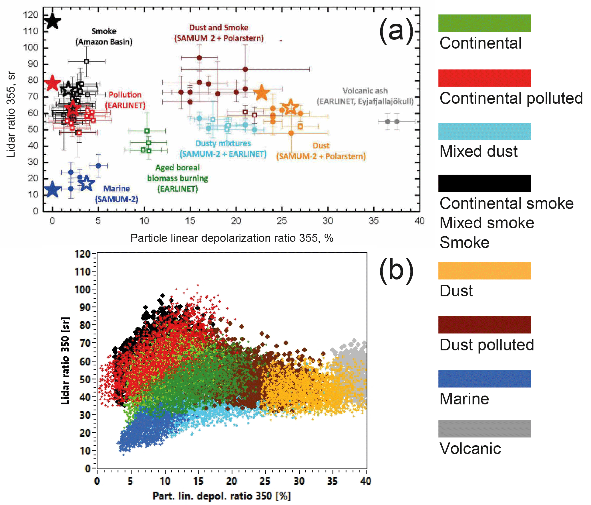
Figure 5Lidar ratio versus particle linear depolarization ratio. (a) Synthesis of ground-based observations and simulations adapted from Wandinger et al. (2016) (their Fig. 1). Filled stars represent simulations using the components of Aerosol CCI and variations with different refractive indexes and shape distributions (open stars). (b) Synthetic data from the NATALI aerosol model.

Download

Wandinger et al. (2016) provided a synthesis of ground-based observations of lidar ratio and particle linear depolarization at 355 nm for different aerosol types (i.e. dust, smoke, pollution, marine, aerosol, volcanic ash) and mixtures, collected during a series of measurement campaigns, i.e. PollyXT measurements at Cabo Verde (Groß et al., 2011), at EARLINET stations of Leipzig and Munich (Groß et al., 2012), in the Amazon Basin (Baars et al., 2012), and on board Polarstern over the North Atlantic (Kanitz et al., 2013) (Fig. 5a). The synthetic data show a wider spread because of large uncertainty accepted for the input parameters. Very high values for the linear depolarization for smoke in the Aerosol CCI (European Space Agency Aerosol Climate Change Initiative) could not be achieved in the aerosol model (Fig. 5b).

When the entire output of the aerosol model is considered (i.e. 14 aerosol types) there is a high overlap between clusters, in particular for mixtures, due to the built-in uncertainty (Fig. 6a). Smoke and continental pollution almost completely overlap (Fig. 6a), which is consisted with measurements reported in literature (Table 6). This makes the typing challenging. The importance of particle depolarization shown relatively recently (Freudenthaler et al., 2009) can improve the aerosol typing (Fig. 6b). Particle depolarization contributes to the identification of complex mixtures and to the differentiation between mineral and volcanic particles. The main issue for particle depolarization is calibration, having been recently addressed (Belegante et al., 2018; McCullough et al., 2017) and thus few data sets satisfy the depolarization ratio quality criteria for aerosol typing. However, even without particle depolarization information, the low-resolution typing can identify the predominant aerosol types in a mixture.

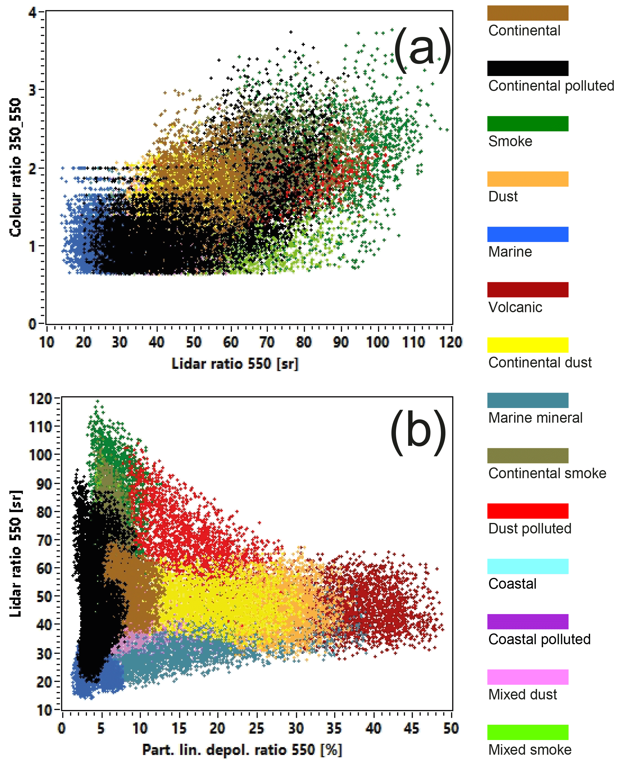
Figure 6Synthetic data set with (a) colour ratio versus lidar ratio, and (b) lidar ratio versus linear particle depolarization ratio using the NATALI classification.

Download

3.2 ANN performance

Figure 7 shows the overall performances of the ANNs for the high-resolution typing (i.e. A1H, A2H, A3H) and low-resolution typing (i.e. A1L, A2L, A3L). In high-resolution typing at least 70 % of the aerosol types defined (i.e. 10 out of 14) should be correctly assessed in more than 75 % of the cases with a confidence higher than 0.7. In low-resolution typing at least 70 % of the predominant aerosol types (i.e. 4 out of 5) defined should be correctly assessed in more than 65 % of the cases with a confidence higher than 0.7.

The aerosol type is recognized in more than 96 % of all cases in high-resolution typing (Fig. 7a). The missed cases are, in general, due to the complete overlap between the input parameters. For example, continental smoke is classified as smoke in 22 % of the missed cases (i.e. 1.9 % of the total number of cases); continental dust is classified as dust in 9 % of the missed cases (i.e. 0.3 % of the total number of cases). Note that 33 % of the missed cases (1.2 % of the total number of cases) are classified as unknown.

The predominant aerosol is recognized in more than 91 % of the cases in low-resolution typing (Fig. 7b). Most of the missed cases are due to the ANNs not being able to distinguish between continental aerosol and smoke, and continental-polluted aerosol (i.e 36 % of the missed cases representing 3.2 % of the total number of cases), and between continental, smoke and marine aerosols, and continental-polluted aerosols (i.e. 35 % of the missed cases, 3.1 % of all cases). Continental-polluted and marine aerosols are sometimes identified by the ANNs as continental (i.e. 27 % of all missed cases, 2.4 % of the total number of cases).

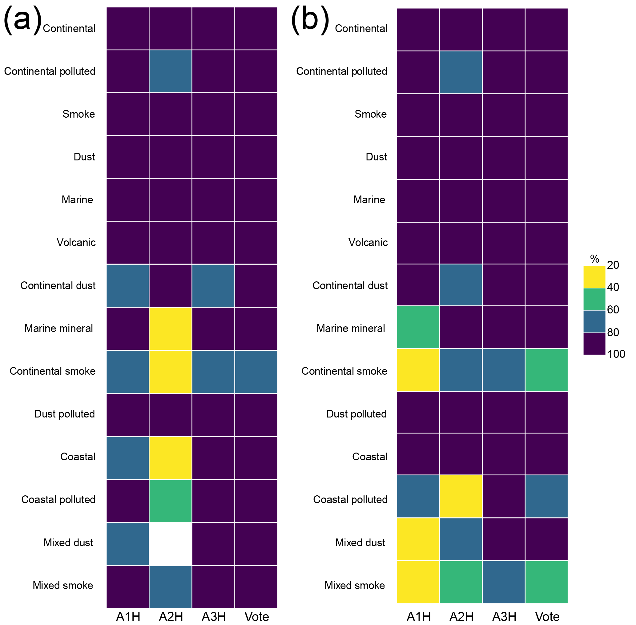
Figure 7Performances of ANNs for (a) high-resolution typing and (b) low-resolution typing for each ANN (i.e. A1H, A2H, A3H) and the combine results (vote) of the three ANNs. The intervals of ANN confidence levels are shaded according to the scale.

Download

A3H and A3L were the best-performing ANNs but did not always have a high confidence level (Fig. 7). A2H and A2L have the lowest performances, but they can help in certain cases, for example in recognizing continental-dust aerosols. The voting procedure does not always provide the right answer, for example when A3H provides the correct typing but its confidence level is low.

The dependence of the aerosol typing on RH shows that the performances of the ANNs are decreased with an increase in RH, only for continental-smoke and continental-dust for high-resolution typing (Fig. 8) and for continental smoke and mixed smoke for low-resolution typing (Fig. 8). Pure aerosol types are recognized for all values of RH. For coastal polluted, the relative humidity increase results in an increase of typing performance. Overall, lower performances are obtained in low-resolution typing.

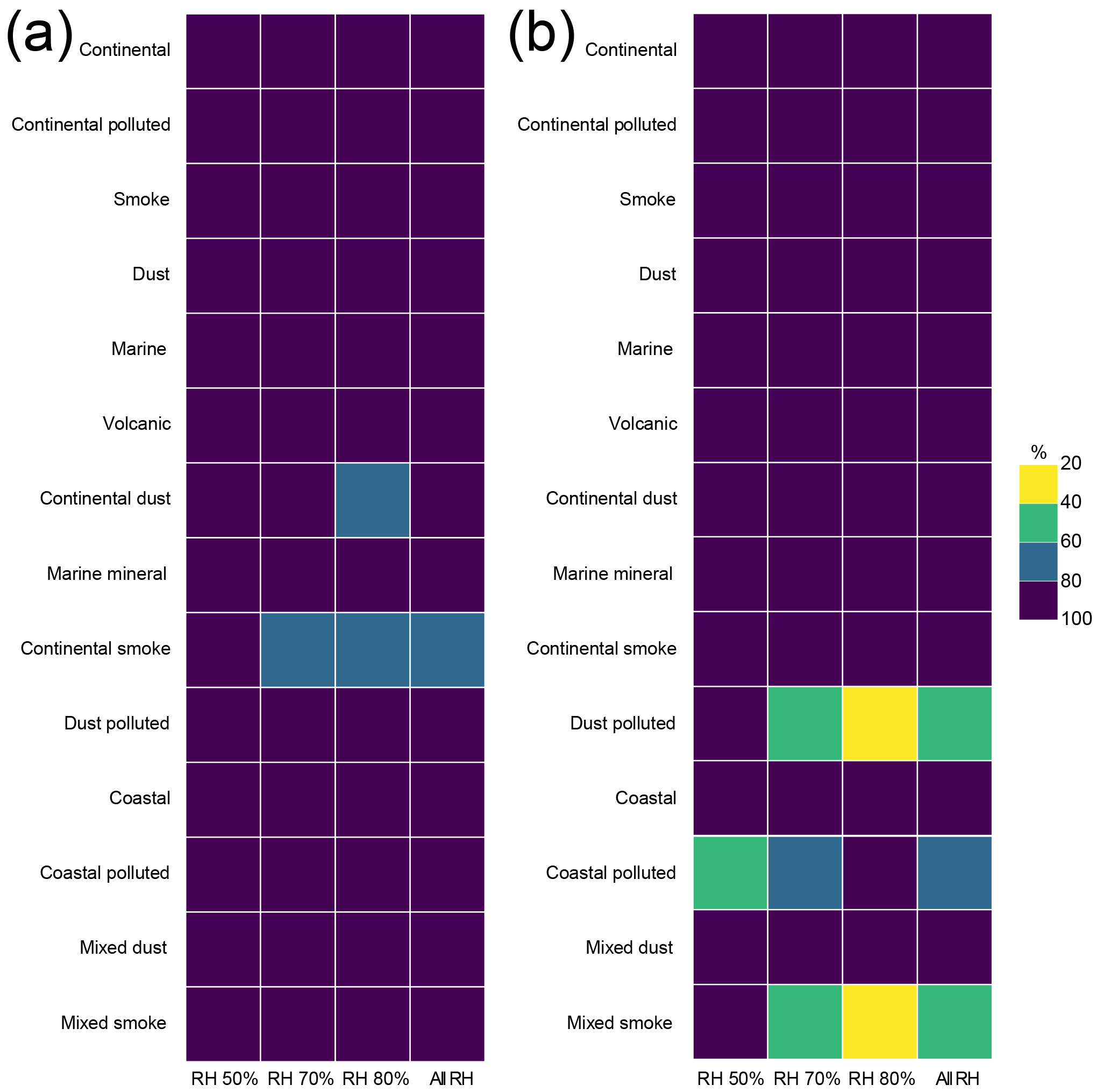
Figure 8Performances of the ANNs for different relative humidity values (i.e. 50 %, 70 %, 80 %) for (a) high-resolution typing and (b) low-resolution typing. The intervals of ANN confidence levels are shaded according to scale.

Download

3.3 Comparison with EARLINET-CALIPSO classification

Observational data from EARLINET Data Base (https://www.earlinet.org/index.php?id=earlinet_homepage, last access: 18 September 2018), related to the CALIPSO (Cloud-aerosol Lidar and Infrared Pathfinder Satellite Observation) overpasses over different EARLINET observational sites, were compared with the synthetic data obtained from the aerosol model. The EARLINET-CALIPSO database (Pappalardo et al., 2010), covers the data of 2000–2018 and includes a total of 718 cases and 21 aerosol and cloud types. Only 13 of these cases contained all of the necessary parameters (i.e. 3 backscatters, 2 extinctions and 1 depolarization). In general, the missing parameter is the particle depolarization. To increase the number of cases, the particle depolarization was added assuming values reported in literature as typical for the corresponding aerosol type. This way, 105 cases containing all needed parameters were obtained. The cases for which all parameters were within 20 % of relative error were selected (63 cases), whereby 57 corresponded to known aerosol types.

Additionally, profiles available at the EARLINET site in Bucharest/Măgurele, established by the Romanian National Institute for Research and Development of Optoelectronics (INOE), were used to increase the validation measurement sample. The INOE database contains 464 measurement sets performed with the multiwavelength Raman depolarization Lidar (Belegante et al., 2011) between June 2012 and September 2014. About 44.6 % of measurements were conducted at night-time (including the Raman-derived extinction coefficient profiles). Out of these, 871 processed layers containing backscattering, extinction and particle depolarization profiles averaged over 1 h. Only layers with significant loads (i.e. layers for which the uncertainty of the retrieved optical parameters is below the limits accepted by the algorithm) were selected, for which all intensive parameters were retrieved with accuracies higher than 20 %. Mean values within each layer were computed, excluding the edges of the layers, where the smoothing introduces large errors due to the high gradients. For each layer, the Ångström exponent, colour ratio, colour index, lidar ratio, and linear particle depolarization ratio were computed. Thresholds were then used to estimate the type of aerosol at first glance, which resulted in a data set with 311 layers accepted by the algorithm, of which for only 182 layers of auxiliary data were available. Auxiliary data were used to compare the results of the typing.

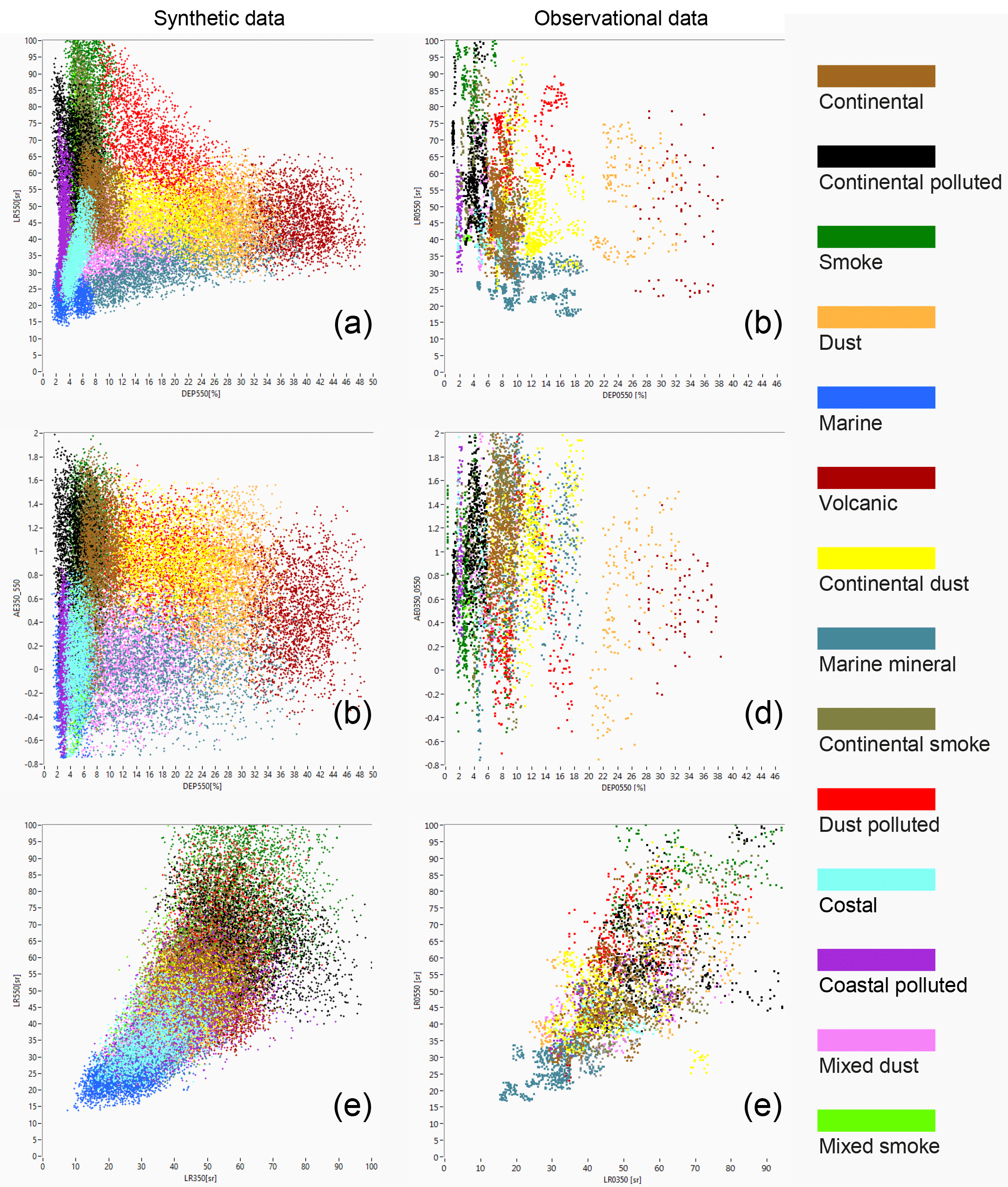
Figure 9Results of the aerosol typing from NATALI aerosol model (synthetic data) and observations (observational data, EARLINET-CALIPSO database and additional data sets collected at the EARLINET station in Bucharest). (a, b) Lidar ratio and particle depolarization (VIS), (c, d) Ångström exponent and particle depolarization (VIS), and (e, f) lidar ratio (VIS) and lidar ratio (UV).

Download

The time series of lidar measurements (532 nm volume depolarization and 355, 532, and 1064 nm range corrected signals) were used to identify the aerosol layers. The identification of the aerosol source was based on 96 h backward trajectories using HYSPLIT (Stein et al., 2016). The source was assumed to originate at the region where the trajectory was closest to the ground, providing guidance for identifying possible emission sources. The rainfall along the trajectory was used as an indicator of likely wet deposition. A synoptic diagnosis of the main meteorological file (e.g. pressure, geopotential height, temperature, relative humidity, wind), based on NCEP/NCAR Reanalysis (Kalnay et al., 1996), was used to confirm the aerosol trajectories and to determine the type of atmospheric circulation, weather regimes, and weather phenomena along the trajectories.

Figure 9 shows the comparison between the aerosol typing based on the aerosol model (synthetic data) and the EARLINET-CALIPSO and INOE database (observed data). The large spread of the measured parameters is caused by the mixtures of three components, incorrect calibration, or inappropriate estimation of aerosol type. On the other hand, the sparse observational data led to apparently incomplete clusters. No conclusions can be drawn for marine aerosols, as they are not represented in the observational data.

Low values are observed in the Ångström exponent for several cases of dust polluted and smoke categories, as well as low values for the 532 nm lidar ratio are seen for several cases of continental and continental-dust types, indicating a small portion of marine particles. This is most likely due to the fact that particles are transported over a short distance above the sea before reaching the target and thus are misclassified. The high values for the Ångström exponent for some of the marine mineral aerosols indicate a mixture with smoke. Values of the Ångström exponent greater than 1.8, measured for smoke and continental-polluted aerosols, failed to be simulated. Actually, in general, the agreement of classification of the simulated data and the real observations is very good, given all limitations discussed.