the Creative Commons Attribution 4.0 License.
the Creative Commons Attribution 4.0 License.
 | 10 Oct 2018
Atmospheric oxidation in the presence of clouds during the Deep Convective Clouds and Chemistry (DC3) study
Xinrong Ren
Li Zhang
Jingqiu Mao
David O. Miller
Bruce E. Anderson
Donald R. Blake
Ronald C. Cohen
Glenn S. Diskin
Samuel R. Hall
Thomas F. Hanisco
L. Gregory Huey
Benjamin A. Nault
Jeff Peischl
Ilana Pollack
Thomas B. Ryerson
Taylor Shingler
Armin Sorooshian
Kirk Ullmann
Armin Wisthaler
Paul J. Wooldridge
Deep convective clouds are critically important to the distribution of atmospheric constituents throughout the troposphere but are difficult environments to study. The Deep Convective Clouds and Chemistry (DC3) study in 2012 provided the environment, platforms, and instrumentation to test oxidation chemistry around deep convective clouds and their impacts downwind. Measurements on the NASA DC-8 aircraft included those of the radicals hydroxyl (OH) and hydroperoxyl (HO2), OH reactivity, and more than 100 other chemical species and atmospheric properties. OH, HO2, and OH reactivity were compared to photochemical models, some with and some without simplified heterogeneous chemistry, to test the understanding of atmospheric oxidation as encoded in the model. In general, the agreement between the observed and modeled OH, HO2, and OH reactivity was within the combined uncertainties for the model without heterogeneous chemistry and the model including heterogeneous chemistry with small OH and HO2 uptake consistent with laboratory studies. This agreement is generally independent of the altitude, ozone photolysis rate, nitric oxide and ozone abundances, modeled OH reactivity, and aerosol and ice surface area. For a sunrise to midday flight downwind of a nighttime mesoscale convective system, the observed ozone increase is consistent with the calculated ozone production rate. Even with some observed-to-modeled discrepancies, these results provide evidence that a current measurement-constrained photochemical model can simulate observed atmospheric oxidation processes to within combined uncertainties, even around convective clouds. For this DC3 study, reduction in the combined uncertainties would be needed to confidently unmask errors or omissions in the model chemical mechanism.
- Article
(6093 KB) -
Supplement
(11083 KB) - BibTeX
- EndNote


Deep convective clouds alter the chemical composition of the middle and upper troposphere (Chatfield and Crutzen, 1984). At its base, a cloud ingests air containing volatile organic compounds (VOCs) and anthropogenic pollutants emitted into the atmospheric boundary layer, lifts it to the upper troposphere where it spreads into the anvil, and is eventually mixed with the surrounding air, including some from the lower stratosphere. Inside the convective cloud, the chemical composition is transformed: boundary layer air is diluted with cleaner midlatitude air; water-soluble chemical species are scrubbed by contact with cloud particles; and nitrogen oxides are added by lightning. At the same time, shading in the cloud core extends the lifetime of certain photochemically active compounds. This transformed chemical composition profoundly alters the atmospheric oxidation in the upper troposphere.
Atmospheric oxidation is driven primarily by hydroxyl (OH), whose concentration is strongly dependent on ozone (O3), especially in the upper troposphere (Logan et al., 1981). Ozone is a source of OH through its destruction by solar ultraviolet radiation, which produces an excited state oxygen atom that can react with water vapor to produce OH. Hydroxyl reactions with methane (CH4) and VOCs produce oxygenated volatile organic compounds (OVOCs), including organic peroxyl (RO2, where R=CH3, C2H5, …) and hydroperoxyl (HO2). At the same time, OH reacts with carbon monoxide to produce HO2. The reaction of these peroxyls with NO creates new nitrogen dioxide (NO2), which then absorbs solar radiation to produce NO and O(3P), and O(3P) combines with O2 to form new O3. In the absence of nitrogen oxides (), the formation of OH and HO2 acts to destroy O3 through OH production and the reactions O3+HO2 and O3+OH. Thus, atmospheric oxidation is strongly dependent on the chemical composition of the air exiting deep convective clouds.
Deep convective clouds transform the chemical composition of the upper troposphere in several ways (Barth et al., 2015, and references therein). NOx produced by lightning can have mixing ratios of several parts per billion (ppbv) in the anvil downwind of convection (Ridley et al., 1996; Schumann and Huntrieser, 2007; Pollack et al., 2016; Nault et al., 2017). In addition to long-lived chemical species such CH4, carbon monoxide (CO), and alkanes, short-lived chemical species such as isoprene and its reaction products or those found in fire plumes can be rapidly transported from the planetary boundary layer (PBL) by convection into the upper troposphere (Apel et al., 2012, 2015). Convection also provides cloud particle liquid and solid surfaces, which can interact with gas-phase chemical species such as peroxides, potentially scrubbing some chemical species from the gas phase, thereby altering the gas-phase chemistry and its products (Jacob, 2000; Barth et al., 2016). The mixture of organics and nitrogen oxides forms organic nitrates, which act as sinks for both organic and hydrogen radicals and nitrogen oxides (Nault et al., 2016). This mixture of organic and hydrogen peroxyl and nitrogen oxides is calculated to enhance upper tropospheric O3 production in the range of 2–15 ppbv day−1 (Pickering et al., 1990; Ren et al., 2008; Apel et al., 2012; Olson et al., 2012). Much of upper tropospheric OH and HO2 is produced by the photolysis of oxygenated chemical species such as formaldehyde (CH2O) and peroxides, which are products of organic chemical species that were lofted into the upper troposphere (Jaeglé et al., 1997; Wennberg et al., 1998; Ravetta et al., 2001; Ren et al., 2008).
Aircraft observations of tropospheric OH and HO2 have been compared to photochemical box models constrained by other simultaneous measurements (Stone et al., 2012). In the planetary boundary layer, measurements of HO2 (Fuchs et al., 2011) and, in some instruments, measurements of OH (Mao et al., 2012) are affected by interferences due predominantly to high abundances of alkenes and aromatics. In the free troposphere, where the abundances of these chemical species are much lower, measured and modeled OH and/or HO2 often agreed to within their combined uncertainties, which are similar to those for ground-based studies (Chen et al., 2012; Christian et al., 2017), but in most of these studies, either modeled and measured OH or HO2 inexplicably disagreed beyond combined model and measurement uncertainty for certain altitudes or chemical compositions (Mauldin III et al., 1998; Faloona et al., 2004; Tan et al., 2001; Olson et al., 2004, 2006, 2012; Ren et al., 2008, 2012; Stone et al., 2010; Kubistin et al., 2010; Regelin et al., 2013).
Only a few studies included OH and HO2 measurements to test the impact of deep convective clouds on atmospheric oxidation in the upper troposphere. During the First Aerosol Characterization Experiment (ACE-1), modeled OH was 40 % greater than measured OH in clouds, possibly due to uptake of OH or HO2 on the cloud particles (Mauldin III et al., 1998). In a different study, downwind of persistent deep convective clouds over the United States, the ratio of measured-to-modeled HO2 increased from approximately 1 below 8 km altitude to 3 at 11 km altitude, suggesting an unknown source of HOx () coming from the nearby convection (Ren et al., 2008). During the African Monsoon Multidisciplinary Analyses (AMMA) campaign, daytime HO2 observations were generally simulated with a photochemical steady-state model, but not in clouds, where modeled HO2 greatly exceeded observed HO2 (Commane et al., 2010), suggesting HO2 uptake on liquid cloud drops.
Heterogeneous chemistry on aerosol can impact OH and HO2 abundances (Burkholder et al., 2015, and references therein). Typical OH and HO2 accommodation coefficients used in global models are 0.2 on aerosol particles and 0.4–1.0 on ice. Results from a study over the North Atlantic Ocean indicated that the lower observed-than-modeled HO2 could be resolved by including heterogeneous HO2 loss (Jaeglé et al., 2000), but this loss did not resolve the same difference in clear air. This result differs from an analysis of in-cloud measurements over the western Pacific, which provides evidence that uptake in ice clouds has little impact on HO2 (Olson et al., 2004). However, in the same study, the observed-to-modeled HO2 during liquid cloud penetrations was on average only 0.65, compared to 0.83 outside of clouds, and this difference depended upon both the duration of the cloud penetration and the liquid water content (Olson et al., 2006). The uptake of HO2 in liquid cloud particles was also observed by Whalley et al. (2015).
Laboratory studies show that the HO2 effective uptake coefficient for moist aerosol particles that contain copper is probably much lower than 0.01 in the lower troposphere but may be greater than 0.1 in the upper troposphere (Thornton et al., 2008). However, other laboratory studies show that adding organics to the particles or lowering the relative humidity can reduce uptake coefficients (Lakey et al., 2015, 2016). These values are generally lower than the HO2 effective uptake coefficient assumed in global chemical transport models. On ice surfaces, the OH uptake coefficient is thought to be at least 0.1 and probably larger (Burkholder et al., 2015). In global models, metal catalyzed HO2 destruction on aerosol particles can reduce global HO2 in a way that is more consistent with observed OH and HO2 (Mao et al., 2010). More recently, a global sensitivity analysis shows that modeled HO2 is most sensitive to aerosol uptake at high latitudes (Christian et al., 2017), consistent with the conclusion of Mao et al. (2010).
In this paper, we focus on the comparison of measured and modeled OH and HO2 near deep convective clouds and the implications of this comparison. Our goal is to test the understanding of atmospheric oxidation around deep convective clouds and in the cloud anvils. One possible effect is heterogeneous uptake of OH, HO2, and RO2 around and in these clouds, which could alter OH and HO2. The data for this analysis were collected during the Deep Convective Clouds and Chemistry (DC3) study in 2012.
2.1 The DC3 study
Barth et al. (2015) provide a detailed description of the objectives, strategy, locations, instrument payloads, and modeling for DC3. DC3 was designed to quantify the link between the properties of deep convective clouds and changes in chemical composition in the troposphere. This section provides information on the aspects of DC3 that relate most directly to the measured and modeled OH, HO2, and OH reactivity.
DC3 involved several heavily instrumented aircraft, ground-based dual Doppler radar, lightning mapping arrays, and satellites (Barth et al., 2015). Studies were generally focused on areas in Colorado, Texas/Oklahoma, and Alabama that had dual Doppler radar coverage to quantify cloud properties. The field study took place in May–June 2012. The aircraft were based in Salina, Kansas, which was central to the three main target regions in Colorado, Texas/Oklahoma, and Alabama. The NASA DC-8 sampled deep convection six times in Colorado, four times in Texas/Oklahoma, and three times in Alabama. Typically working with the National Science Foundation (NSF) Gulfstream V (GV) aircraft, the DC-8 would sample the inflow region to a growing cumulus cloud and then after it formed, spiral up to the anvil height (∼8–12 km) and join the NSF GV in sampling the outflow region of the same convection.
In addition, during the night before 21 June, the outflow from a mesoscale convective system (MCS) in the Midwest spread over Iowa and Missouri and then into Illinois and Tennessee. The DC-8 sampled the outflow of this MCS starting at sunrise of 21 June, flying six legs, each approximately 400 km long, across the outflow roughly perpendicular to the wind and adjusting the downwind distance to account for the outflow velocity (Nault et al., 2016). The southern two-thirds of the first three legs were in a thin cirrus cloud and the rest was clear.
Most DC3 flights began in the late morning in order to be in position to sample near active deep convection occurring in the late afternoon and concluded near dusk for safety. About 90 % of the flight time occurred when the solar zenith angle was less than 85∘. Only the photochemical evolution flight on 21 June began before dawn.
The NASA DC-8 aircraft was the only aircraft that had an instrument to measure OH and HO2. The DC-8 payload was quite comprehensive, thus providing detailed chemical composition, particle characteristics, and meteorological parameters to constrain the photochemical box model that is used to compare observed and modeled OH and HO2. Direct comparison between observed and modeled OH and HO2 is valid because the lifetimes of OH and HO2 are short: a few seconds or less for OH and a few tens of seconds for HO2. Thus, the analyses in this paper use only measurements from the DC-8.
2.2 Measurement of hydroxyl (OH) and hydroperoxyl (HO2)
OH and HO2 were measured with the Penn State Airborne Tropospheric Hydrogen Oxides Sensor (ATHOS), which uses laser-induced fluorescence (LIF) in low-pressure detection cells (Hard et al., 1984). ATHOS is described by Faloona et al. (2004). Sampled air is pulled through a 1.5 mm pinhole into a tube that leads to two detection axes. The pressure varies from 12 hPa at low altitudes to 3 hPa aloft. The laser beam is passed 32 times through the detection region with a multi-pass cell set at right angles to the gated microchannel plate detector. As the air passes through a laser beam, OH absorbs the laser radiation (3 kHz repetition rate, 20 ns pulse length) and fluoresces. In the first 100 ns, the signal contains fluorescence as well as scattering from the walls, Rayleigh scattering, and clouds drops. OH fluorescence is detected from 150 to 700 ns after each laser pulse. OH is detected in the first axis; reagent nitric oxide (NO) is added before the second axis to convert HO2 to OH, which is then detected by LIF. The laser wavelength is tuned on resonance with an OH transition for 15 s and off resonance for 5 s, resulting in a measurement time resolution of 20 s. The OH fluorescence signal is the difference between on-resonance and off-resonance signals. The ATHOS nacelle inlet is attached below a nadir plate of the forward cargo bay of the DC-8, and the lasers, electronics, and vacuum pumps were inside the forward cargo bay.
In clouds, cloud particles can be pulled into the detection system and remain intact enough to cause large, short scattering signals in the fluorescence channels randomly during on-resonance and off-resonance periods. Differencing these signals to find OH creates large positive and negative noise, which reduces the measurement precision by as much as a factor of 5. When the background signal due to these cloud particles exceeded the average background signal by 4 standard deviations, the online and offline data were removed from the data set before the analyses were performed. Less than 3 % of the data were removed. The overall results for OH and HO2 vary less than 4 % for filtering between 2 and 6 standard deviations.
The instrument was calibrated on the ground both in the laboratory and during the field campaign. Different sizes of pinholes were used in the calibration to produce different detection cell pressures to mimic different altitudes. Monitoring laser power, Rayleigh scattering, and laser linewidth maintained this calibration in flight. For the calibration, OH and HO2 were produced through water vapor photolysis by UV light at 184.9 nm. Absolute OH and HO2 mixing ratios were calculated by knowing the 184.9 nm photon flux, which was determined with a Cs-I phototube referenced to a NIST-calibrated photomultiplier tube, the H2O absorption cross section, the H2O mixing ratio, and the exposure time of the H2O to the 184.9 nm light. The absolute uncertainty was estimated to be ±16 % for both OH and HO2 at a 1σ confidence level. The 1σ precision for a 1 min integration time during this campaign was about 0.01 parts per trillion by volume (pptv, equivalent to pmol mol−1) for OH and 0.1 pptv for HO2. Further details about the calibration process may be found in Faloona et al. (2004).
For environments with substantial amounts of alkenes and aromatics, ATHOS has interferences for both OH (Mao et al., 2012) and HO2 (Fuchs et al., 2011). New ATHOS measurement strategies have minimized these interferences, but these strategies were not fully developed in time for DC3. However, recent missions have shown that the OH interference is significant only just above forests or cities and is negligible above the PBL. On the other hand, the deep convective clouds encountered in DC3 can lift short-lived VOCs that cause the HO2 interference to the upper troposphere. Because ATHOS was still sensitive to this RO2 interference in DC3, we are not able to determine if this interference is affecting the HO2 observations around and in these clouds. For OH, we will factor in the likelihood that the OH has an interference in the PBL above forests in the discussion comparing observed and modeled OH.
For HO2, the correction method uses more than 1000 RO2 chemical species modeled by the Master Chemical Mechanism v3.3.1 (MCMv3.3.1) and assumes that they are ingested into the detection flow tube without any wall loss. The model then calculates the resulting OH, which is what would be detected as HO2. The calculated concentration of reactant NO is cm−3 and the reaction time was determined to be 3.7 ms, as verified by the HO2 conversion rate measured in the laboratory. This calculation was repeated for each 1 min time step and this calculated interference was then subtracted from the observed HO2, resulting in the HO2 values reported here. Observed HO2 was reduced by an average of 2 %, with some peaks of 10 %, both in the PBL and aloft. Because the model RO2 mechanisms are uncertain, the uncertainty for this correction is estimated to be a factor of 2, which increases the absolute uncertainty for HO2 from ±16 % to ±20 % (1σ confidence).
2.3 Measurement of OH reactivity
The OH reactivity is the sum of the product of OH reactants and their reaction rate coefficients with OH and is the inverse of the OH lifetime. It is directly measured by adding OH to the air flowing through a tube and then monitoring the decay of the logarithm of the OH signal as the reaction time between the OH addition and OH detection is increased (Kovacs and Brune, 2001). OH can also be lost to the tube walls, so the measured OH reactivity must be corrected for this wall loss. The OH reactivity can be determined with Eq. (1).
[OH]0 is the initial OH concentration, [OH] is the [OH] concentration after a reaction time Δt between OH and its reactants, and kwall is the OH wall loss.
The OH reactivity is measured with the OH reactivity instrument (OHR), which sits in a rack in the DC-8 forward cargo (Mao et al., 2009). Ambient air is forced into a flow tube (10 cm diameter) at a velocity of 0.3–0.7 m s−1, flows past the pinhole of an OH detection system similar to the one used for ATHOS, and then is expelled out of the aircraft. In a movable wand in the center of the flow tube, OH is produced by the photolysis of water vapor by 185 nm radiation and then injected into the flow tube, mixing with the ambient air flow. As the wand is pulled back, the distance between the injected OH and the OH reactants in the air increases, resulting in the OH decay. The distance divided by the measured velocity gives the reaction time. The wand moves 10 cm in 12 s and then returns to the starting position, measuring a decay every 20 s.
The OHR calibration was checked in the laboratory before and after DC3 using several different known amounts of different chemical species. During a semiformal OHR intercomparison in Jülich, Germany, in October 2015, the OHR instrument was combined with a different laser, wand drive, and electronics, and despite the difficulties encountered, it was found to produce accurate OH reactivity measurements (Fuchs et al., 2017).
The uncertainty in the OH reactivity measurement consists of an absolute uncertainty and the uncertainty associated with the wall loss subtraction. Changes in the OHR instrument between Arctic Research of the Composition of the Troposphere from Aircraft and Satellites (ARCTAS) and DC3 result in slightly different instrument operation, wall loss, and measurement uncertainties between this paper and Mao et al. (2009). The pressure dependence of the OH wall loss was measured in the laboratory using ultra zero air (99.999 % pure) and was found to be between 2 and 4 s−1 over the range pressures equivalent to 0 to 12 km altitude. The flow tube wall is untreated aluminium so that every OH collision with the wall results in complete OH loss no matter the environment or altitude. Mao et al. (2009) confirm the zero found in the laboratory agrees with the zero found in flight. From these laboratory calibrations, the estimated uncertainty in the wall loss correction is ±0.5 s−1 (1σ confidence). When the OH reactivity is 1 s−1, the combined uncertainty from the absolute uncertainty and the zero decay is ±0.6 s−1 (1σ confidence), which suggests that 90 % of the measurements should be within ±1.2 s−1 of the mean value.
Air entering the OHR flow tube was warmed by ∼5 ∘C at altitudes below 2 km to by as much as 75 ∘C at 12 km. The flow tube pressure was 50 hPa greater than ambient due to the ram force pushing air through the flow tube. These temperature and pressure differences can affect the reaction rate coefficients for some OH reactants and thus change the OH reactivity. In order to compare observed and model-calculated OH reactivity, the model was run for both ambient conditions and for the OHR flow tube pressure and temperature, but the observed and model-calculated OH reactivity will be compared for the OHR flow tube pressure and temperature.
2.4 Measurement of other chemical species, photolysis frequencies, and other environmental variables
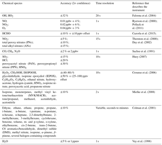
Accurate measurements of other chemical species and environmental variables are critical for this comparison of measured and modeled OH, HO2, and OH reactivity. The photolysis frequency measurements are particularly critical for DC3 because of all the time spent flying around clouds and in the deep convection anvil. A list of these measurements is given in Table 1 and is summarized in Barth et al. (2015, 2016) and Pollack et al. (2016). The list of measured chemical species includes CO, CH4, N2O, NO, NO2, O3, organic nitrates, alkanes, alkenes, aromatics, aldehydes, alcohols, and peroxides.
2.5 Photochemical box model
The photochemical box model used in this study is based on the Matlab-based modeling framework, the Framework for Zero-Dimensional Atmospheric Modeling (F0AM), which was developed and made freely available by Glenn Wolfe (Wolfe et al., 2016). The gas-phase photochemical mechanism was MCMv3.3.1 (Saunders et al., 2003; Jenkin et al., 2003). This model was constrained by all simultaneous measurements of chemical species, photolysis frequencies, and meteorological variables (Table 1) and then run to calculate OH, HO2, and all reaction products that were not measured, such as organic peroxy radicals. Pernitric acid (HO2NO2) was measured but was not used to constrain the model because few measurements were reported below 4 km. Measured and modeled HO2NO2 agree to within ∼25 % from 5 to 9 km, and modeled HO2NO2 is 1.7 times that measured above 8 km. This difference between using modeled and observed HO2NO2 made only a few percent difference in modeled OH and HO2.
A publicly available merge file provided the constraining measurements for the photochemical model (Aknan and Chen, 2017). We chose the 1 min merge as a compromise between higher-frequency measurements that needed to be averaged into 1 min bins and lower-frequency measurements that needed to be interpolated between 1 min bins. OH and HO2 measurements, made every 20 s, were averaged into the 1 min bins.
Heterogeneous chemistry was added to the model for some model runs. While many chemical species undergo heterogeneous chemistry, most of the chemical species that strongly influence OH and HO2 were measured so that their heterogeneous chemistry can be ignored in these comparisons between observed and modeled OH and HO2. However, organic peroxyl radicals were not measured and their heterogeneous chemistry could have an influence on OH and HO2. Thus, heterogeneous chemistry is implemented in the model for OH, HO2, and RO2, even though the uptake of RO2 is thought to be small.
The common types of particles encountered with convection are humidified submicron aerosol particles around and in the convection, liquid drops in lower-altitude clouds, and ice particles in the deep convective cloud anvil. The effective uptake of OH, HO2, and RO2 onto these surfaces was found from Eq. (2).
γeff is the effective uptake coefficient, γsurface is surface reaction uptake, α is the accommodation coefficient, γsol is uptake due to diffusion through the liquid, γrxn is uptake due to aqueous-phase reactions, and the last term is the inverse of the gas-phase diffusion in terms of the Knudsen number, Kn (Burkholder et al., 2015; Tang et al., 2014). The first term on the right-hand side is the total uptake coefficient, γtotal. The gas-phase molecular diffusion of chemical species to the particle surface can limit the uptake, especially for large accommodation coefficients and large particles.
The total uptake coefficient for OH and HO2 depends on the particle chemical composition, phase, and size (Burkholder et al., 2015). While some particle properties were measured in DC3, there are unknowns in particle composition and uncertainties in trying to calculate the uptake coefficient for each 1 min time step. The goal of including heterogeneous chemistry in the model is to determine if heterogeneous chemistry has a substantial impact on the comparison between the observed and modeled OH and HO2. Thus, we will run the model with fixed values for the total uptake; if the impact on the modeled OH and HO2 is substantial, then we will have to improve the parameterization of the total uptake.
For aerosol particles, the dry aerosol particle radius is multiplied by the growth factor and then the area-weighted median ambient aerosol radius is determined. The surface area is found by summing the surface area in each bin, multiplying by the bin width, and then correcting by the square of the growth factor for each minute. Ice particles are assumed to be spherical and their size distribution is used to determine the median particle radius. The surface area per cm−3 of air is determined by summing the surface area per cm−3 of air multiplied by the bin width, which was provided in the merge file for each minute.
The model is then run for three different primary cases: gas phase with no heterogeneous chemistry (called “no-het”), heterogeneous chemistry (called “het”) with αaer=0.2 (which is consistent with the value used in some global models) and αice=1.0 for OH, HO2, and RO2, and maximum heterogeneous chemistry (called “hetmax”) with αaer=1.0 and αice=1.0. The observed and modeled OH and HO2 are compared for these three cases.
OH reactivity was also modeled for comparison to observed OH reactivity. Modeled OH reactivity was calculated from the measured chemical species plus OH reactants that were not measured but were produced by the photochemical model. Examples of these additional OH reactants are organic peroxy, organic peroxides, and unmeasured aldehydes. Uncertainty in the modeled OH reactivity is estimated to be ±10 % (1σ confidence) (Kovacs et al., 2001).
Uncertainty in the photochemical box model can be assessed with Monte Carlo methods in which model constraints are varied randomly over their uncertainty ranges and then the widths of the resulting distributions for OH and HO2 abundances are used to determine the model uncertainties. If just reaction rate coefficients, photolysis frequencies, and reaction products are varied, the OH and HO2 uncertainties at the 1σ confidence level are typically ±(10–15) % (Thompson and Stewart, 1991; Kubistin et al., 2010; Olson et al., 2012; Regelin et al., 2013). When uncertainties in the measurements used to constrain the model are included, uncertainties at the 1σ confidence level are typically ±20 % or more for both local and global models (Chen et al., 2012; Christian et al., 2017). We use ±20 % uncertainty at the 1σ confidence level for the model uncertainty in this paper, which can be combined with the measurement uncertainty of about ±20 % uncertainty at the 1σ confidence level. We note that the observed-to-modeled difference for statistical significance lies approximately at the sum of the standard deviations of the mean for the observations and model. As a result, the factors of 1.4 and 1∕1.4 serve as indicators for agreement between observed and modeled OH, HO2, and OH reactivity.
We decided to make the comparisons between observations for all DC3 results, including transit from Salina, KS, to the deep convection regions. Using all the data gives a more robust comparison and was found to give comparison results identical to those using data sets restricted to the radar-enhanced sites in Colorado, Texas/Oklahoma, and Alabama near the vicinity of convection. The direct impact of deep convection is also tested by examining the observed-to-modeled comparison as a function of the ice surface area per cm−3 of air. This analysis achieves the goals laid out in the introduction.
The model was run 27 times to test the sensitivity of the calculated OH and HO2 to different factors. First, the chemical mechanism was expanded to include the reactions of CH3O2+OH and C2H5O2+OH (Assaf et al., 2017), and in some cases, reactions of OH with the next 300 most significant RO2 species that comprise 95 % of the modeled RO2 total, assuming a reaction rate coefficient of 10−10 cm−3 s−1. Adding the measured reactions decreased OH by ∼1 % (5 % maximum) and increased HO2 by <1 % (15 % maximum); adding the assumed reactions of OH with other RO2 species changed modeled OH and HO2 by less than 3 %. Second, the decay frequency of the unconstrained modeled oxygenated intermediates was varied from 6 h to 5 days. The resulting modeled OH and HO2 varied by ∼10 % over this range. This decay time serves as a proxy for surface deposition in the planetary boundary layer as well as for recently measured rapid reactions of highly oxidized RO2+RO2 to form peroxides (Bernt et al., 2018). This decay time is highly uncertain. The mean of the model runs using decay times of 6 h, 1 day, and 5 days and using the model mechanism including CH3O2+OH and C2H5O2+OH was used for the comparisons to the measurements.
The DC3 chemical environments dictate the OH and HO2 abundances. Using all the flight data, altitude profiles of NO, CO, O3, and particle surface area were collected into 0.5 km altitude bins and the median values were found (Fig. 1). The radar altitude is used for these comparisons because the surface elevations and thus planetary boundary layer (PBL) are at different pressure altitudes for the Colorado, Texas/Oklahoma, and Alabama regions.

Figure 1Altitude profiles of median NO, CO, O3, and aerosol (purple) and ice (yellow) surface area (SA). Gray points are individual 1 min data, while median values are represented by the lines. These data are for the entire DC3 study.
Median NO exhibits a C-shaped profile with median values near 50 pptv in the planetary boundary layer, a minimum of 10 pptv at 5 km altitude, and a maximum value of 0.5 ppbv above 10 km. NO in the PBL was largely due to anthropogenic pollution; NO aloft was mainly due to a combination of lightning and stratospheric NOx. Median CO slightly decreased from ∼120 ppbv near the surface to ∼80 ppbv at 12 km. Median O3 was 50 ppbv in the PBL and then increased to as much as 100 ppbv near 12 km, likely due to stratospheric ozone influence. The surface area per cm−3 of air of aerosol was 10−6 cm2 cm−3 in the PBL, but was about cm2 cm−3 above that. Median ice surface area was as much as cm2 cm−3, with high variability spanning a factor of 100.
3.1 Comparing HOx observations with the no-het model
Observations will be compared to the no-het model, which should be considered as the base case; the heterogeneous cases will be considered later. When observed and modeled OH and HO2 are plotted against time, model results generally agree with the observed values to within combined uncertainties, with occasional periods in which the observed values can be either much larger or smaller than all the model variants. A plot of this time series of observed and modeled OH and HO2 includes 14 model runs with model integration times varied from 3 to 24 h, dilution frequencies varied from 6 h to 5 days, and with or without including the RO2+OH reaction (Fig. S1 in the Supplement). Another way to examine these results is to plot the observed and modeled values as a function of altitude and other influential chemical species, photolysis frequency, or location.
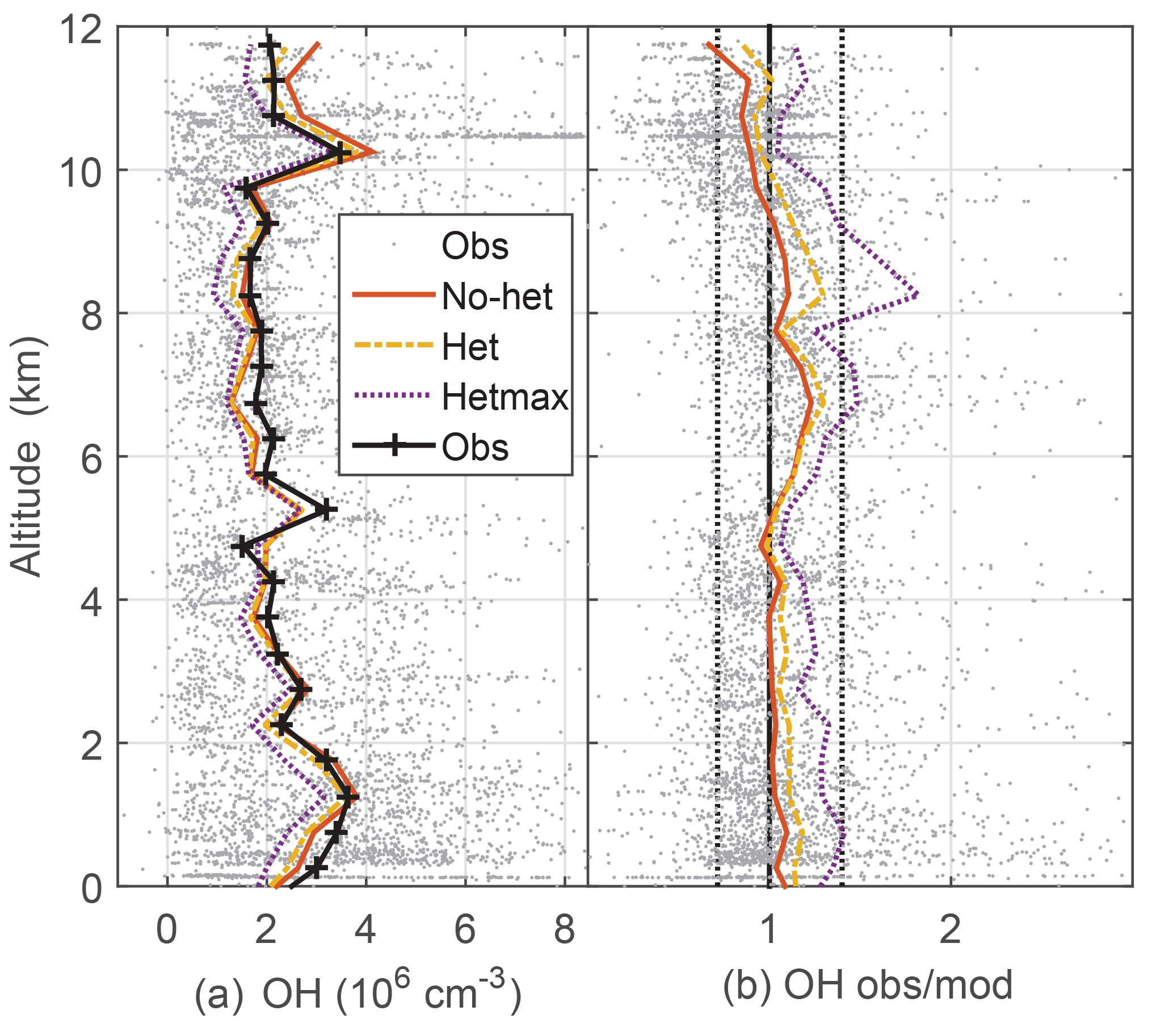
Figure 2Median measured and modeled OH as a function of altitude (a); median ratio of observed-to-modeled OH as a function of altitude (b) for the three models. Gray points are individual 1 min OH observations and ratios of observed to no-het-modeled OH. Dotted vertical black lines on the right (1∕1.4, 1.4) are approximate indicators of measurement–model agreement.
Median observed OH was about 2×106 cm−3 from ∼3 km to 10 km altitude, but was greater than 3×106 cm−3 below 3 km and just above 10 km, where a spike in OH brings the median OH to 3.5×10⁶ (Fig. 2). This profile is consistent with the NO profile; for the NO amounts measured in DC3, increased NO shifts more HOx to OH. The median OH observed-to-modeled ratio for the no-het case is close to 1.0 at 0–4 km, is 1.2–1.3 between 5 and 9 km, and 0.8–0.9 above 10 km. Generally, the observed-to-modeled ratio is within the estimated combined uncertainties described previously. The statistics from scatter plots using a fitting routine that considered uncertainty in both the observations and the model (York et al., 2004) indicate generally good agreement between observed and modeled OH, with the model explaining 85 % of the OH variance (Table 2, Fig. S2).
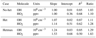
Median observed HO2 was 20–22 pptv below 2 km altitude and decreased almost linearly to 3 pptv at 12 km (Fig. 3). This profile is consistent with the altitude distribution of HOx sources, which are greater near the surface, and, even with convective uplift of oxygenated chemical species such as HCHO, are still much lower than at the surface. Again, the observed-to-modeled ratio is within the estimated combined uncertainties. In addition, the statistics from scatter plots indicate generally good agreement between observed and modeled HO2, with the model explaining 68 % of the HO2 variance (Table 2, Fig. S2). However, the median observed-to-modeled ratio for the no-het case is 1.3 at 1 km altitude, decreases to ∼1 at 5 km, and remains near 1 above 5 km. The ratio of the modeled RO2 to HO2 is typically 1 in the PBL and 0.5 above 5 km. Error in our assumptions for the RO2 interference in the HO2 measurement is a possible cause of the greater observed-to-modeled HO2 below 3 km, but this difference is still well within the combined uncertainty limits.

Figure 3Median measured and modeled HO2 as a function of altitude (a); median ratio of observed-to-modeled HO2 as a function of altitude (b) for the three models. Gray points are individual 1 min OH observations and ratios of observed to no-het-modeled OH. Dotted vertical black lines on the right (1∕1.4, 1.4) are approximate indicators of measurement–model agreement.
An indicator of the HOx cycling between OH and HO2 is the HO2∕OH ratio. If the primary HOx production rate is smaller than the OH–HO2 cycling rate and there is sufficient NO, the HO2∕OH ratio approximately equals the OH loss frequency that cycles OH into HO2 divided by the reaction frequency of HO2 reactions that cycle HO2 to OH, primarily HO2 reactions with NO and O3. Both the observed and modeled HO2∕OH ratios are greater than 100 below 4 km and fall to less than 10 at 12 km (Fig. S3). This profile comes from the greater amount of OH reactants at lower altitudes, which increases the ratio, as opposed to the greater NO amount aloft, which decreases the HO2∕OH ratio. The observed-to-modeled ratio is within the approximate uncertainty limits (1σ confidence) of a factor of 1∕1.4 to 1.4.
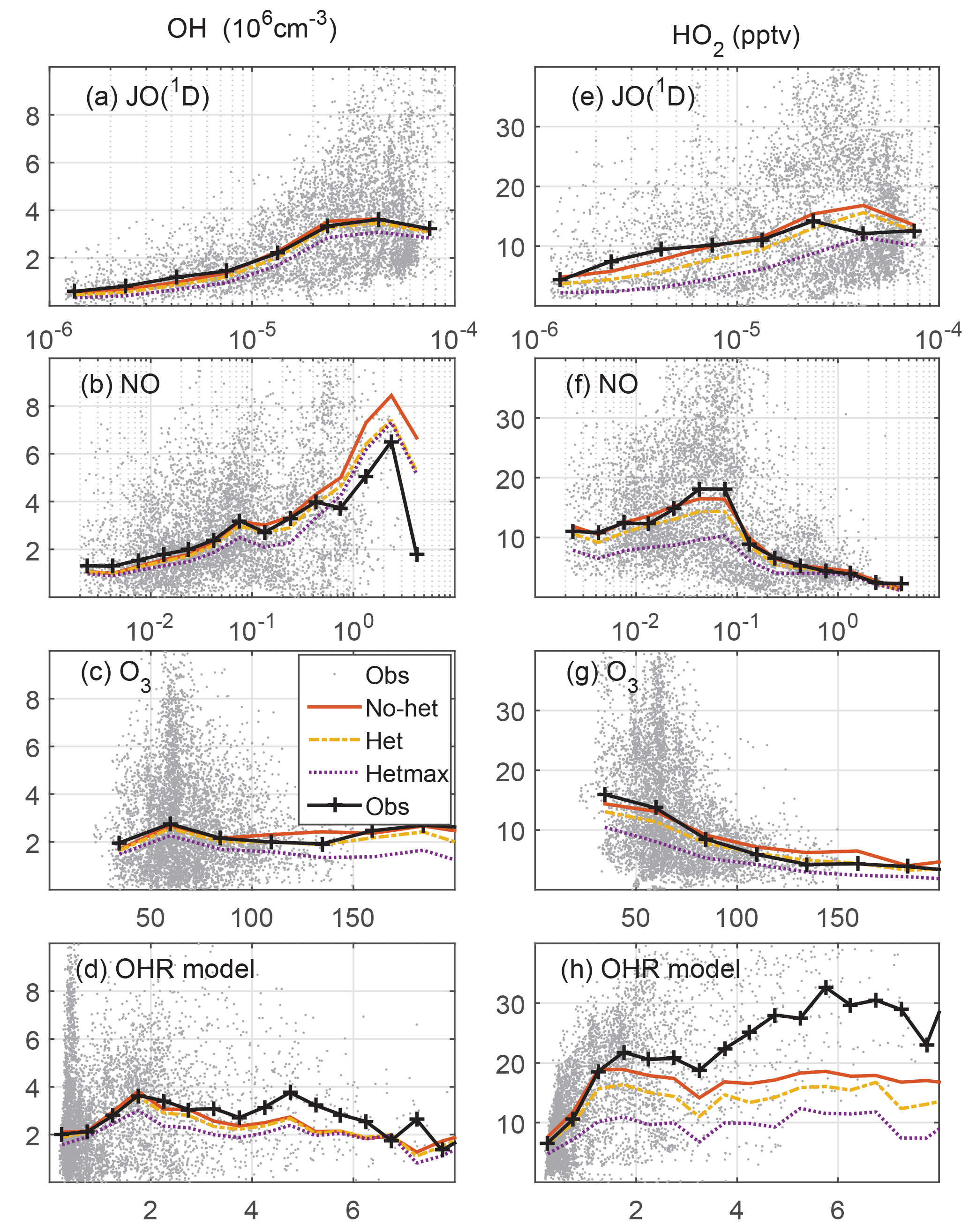
Figure 4Measured and modeled OH (a, b, c, d) and HO2 (e, f, g, h) as a function of controlling variables: JO(1D) in s−1, NO in ppbv, O3 in ppbv, and modeled OH reactivity in s−1. On the left, OH is in units of 106 cm−3; on the right, HO2 is in units of pptv.
Another good test of the model photochemistry is the comparison of observed and modeled OH and HO2 as a function of controlling variables (Fig. 4). The photolysis frequency for O3 producing an excited state O atom, JO(1D), and O3 are both involved in the production of OH. O3 and NO cycle HO2 to OH, while modeled OH reactivity cycles OH back to HO2. In general, measured and modeled OH and HO2 agree from to s−1 for JO(1D), from to ppbv for NO, and from 40 to 100 ppbv for O3. For JO(1D) greater than s−1, the median observed-to-modeled HO2 ratio is 0.98; the in-cloud ratio is an insignificant 10 % less than in clear air, indicating that the observed photolysis frequency measurement is accurate even in clouds. The observed-to-modeled HO2 ratio shows little evidence of a NO dependence, although observed-to-modeled HO2 exceeded 2 for ∼2 % of the values when NO was more than 0.5 ppbv. For the O3 observations greater than 200 ppbv, which are 0.5 % of all observations, the observed-to-modeled HO2 and OH were both ∼0.5. It is possible that the behavior as a function of controlling variables is also a function of altitude. However, with the exception of low values of JO(1D), the median observed-to-modeled OH and observed-to-modeled HO2 are generally independent of both the controlling variables and altitude (Fig. S4). The observed-to-modeled OH and HO2 are also independent of whether the measurements were made in Colorado, Texas/Oklahoma, or Alabama (Fig. S5), although the ratios for some altitudes vary widely due to fewer data points in the altitude medians.
3.2 Comparing OH reactivity observations with the no-het model
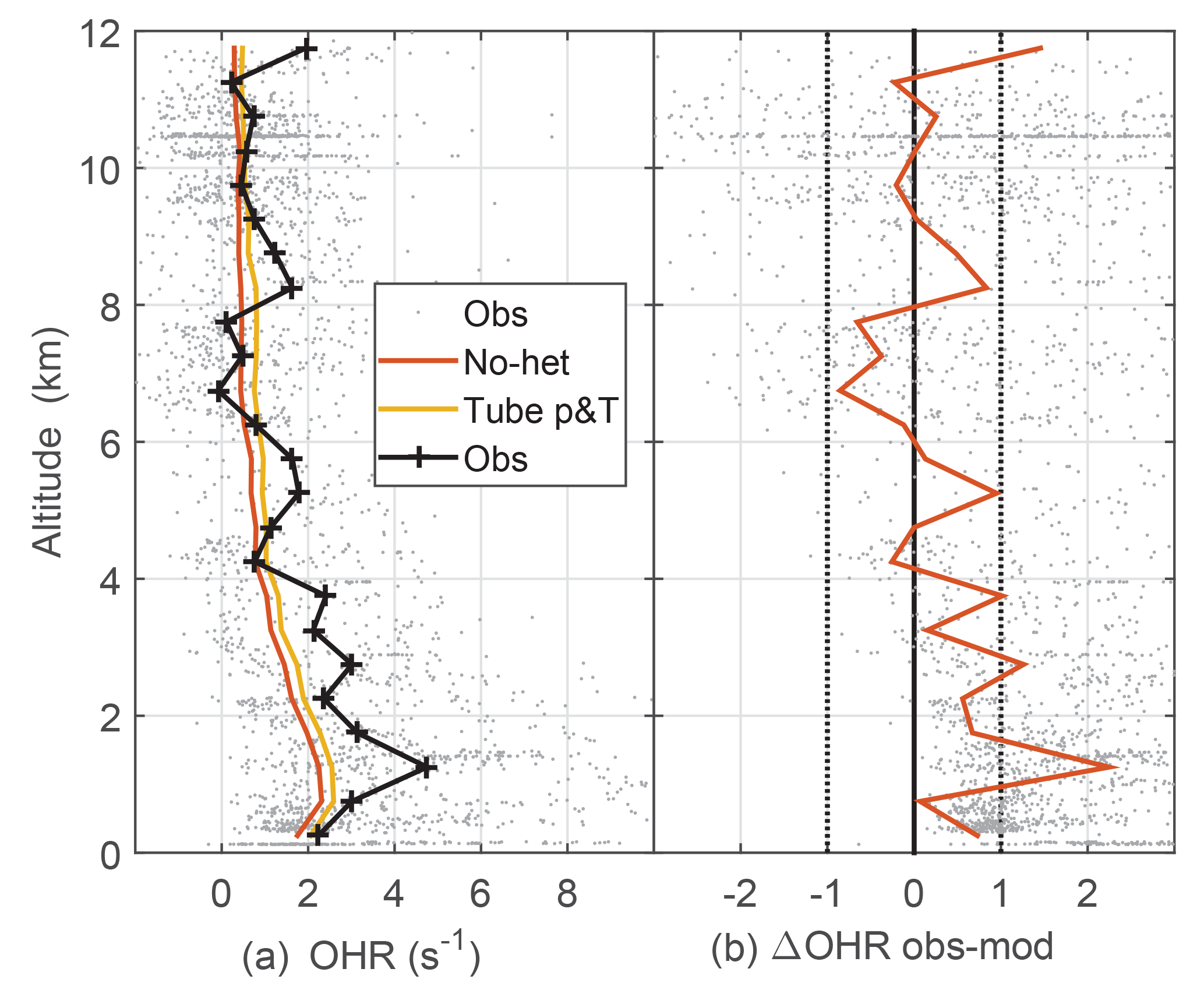
Figure 5Median observed and model-calculated OH reactivity (a) and the difference between observed and modeled OH reactivity (b). The model-calculated OH reactivity was determined for ambient conditions (no-het) and for the OHR flow tube pressure and temperature (tube p&T); see text for explanation. Dotted vertical black lines on the right are approximate indicators of measurement–model agreement.
The measured OH reactivity was typically 2 to 5 s−1 in the PBL but fell to less than 1 s−1 at 12 km altitude (Fig. 5). Observed and modeled OH reactivity is in reasonable agreement when considered in the context of the typical limit of detection for OH reactivity (Fuchs et al., 2017). For DC3, limit of detection for 20 s measurements is estimated to be about 0.6 s−1, which means that most OH reactivity measurements were at or below the limit of detection. The modeled OH reactivity for the OHR flow tube temperature and pressure is greater than the modeled OH reactivity for ambient temperature and pressure by about 0.3 s−1 below 2 km and by about 0.2 s−1 above 10 km (Fig. 5). This difference is negligible below 2 km, but grows to a factor of 1.7 at 10 km where the ambient OH reactivity is just 0.2–0.3 s−1. For the entire altitude range, the difference between the observed and modeled OH reactivity is 0.2 s−1 larger for the modeled OH reactivity at OHR flow tube conditions than for the modeled OH reactivity at ambient conditions, a difference that is swamped by the noise in the observed OH reactivity. The median observed OH reactivity is 1–3 s−1 greater than the modeled OH reactivity below 3 km, and this difference could be evidence of missing OH reactivity.
The percent error between the OH reactivity calculated with modeled OH reactants and that calculated from only the measured OH reactants is, on average, less than 4 %. In the PBL over Alabama, the OH reactivity calculated from the model after 1 day of integration was on average 10 % larger than that calculated from the chemical species measurements. In the Colorado and Texas PBL, the average difference was less than 4 %. According to the model calculations, CO contributes the most to the OH reactivity, with ∼20 % in the PBL and 30–40 % aloft. Next is CH4 at (5–10) %, HCHO at (5–10) %, O3 at (2–10) %, CH3CHO at ∼5 %, and isoprene at (1–2) %, except in some PBL plumes where it was as much as 60 %. The most significant 10 chemical species were all measured and account for (60–70) % of the total model-calculated OH reactivity. Thus, for much of DC3, the OH reactivity calculated from the DC3 measurements almost completely comprises the measured OH reactivity.
3.3 Comparing OH production and OH loss
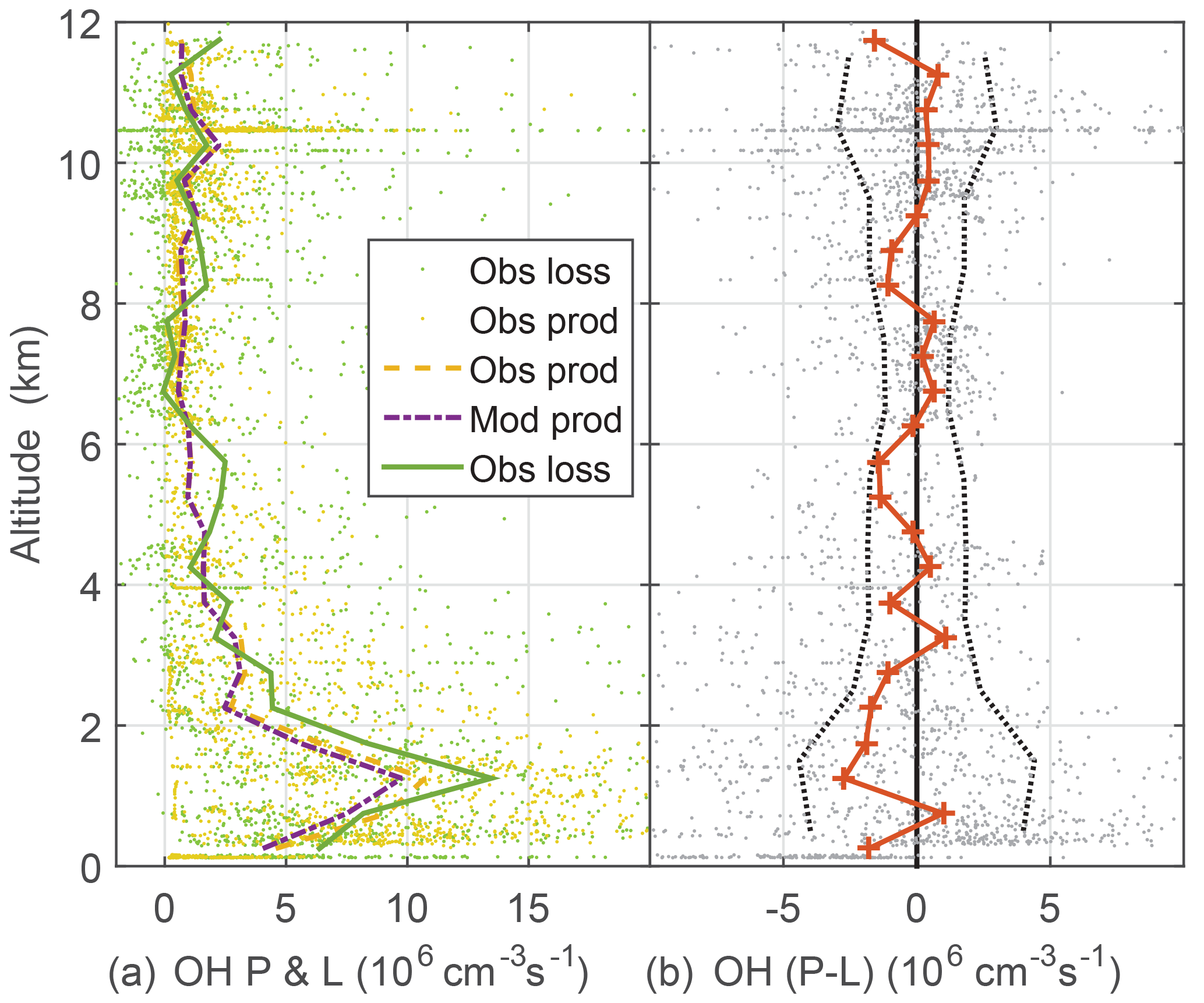
Figure 6OH production and loss (a) and difference between measured OH production and measured OH loss, cm−3 s−1 divided (b). Modeled OH production and loss are equal. Dots are individual 1 min calculations of OH production using observed atmospheric constituents and photolysis frequencies. Dotted vertical black lines on the right are indicators of OH production and loss agreement at the 1σ confidence level and were determined by a propagation of error analysis.
Another critical test of OH photochemistry is the balance between OH production and loss (Fig. 6). The OH lifetime is typically tenths of a second or less in the PBL and a few seconds at high altitude. Thus, for 1 min averages, OH production and loss should essentially be in balance to within the uncertainty estimates from a propagation of error analysis. Modeled OH production and loss are in balance. These uncertainty estimates were obtained by assuming that OH production is dominated by and O3 photolysis followed by reaction of excited state oxygen atoms with water vapor and that the OH loss is given by the OH reactivity multiplied by the OH concentration. The largest contributor to the uncertainty is the zero offset for the OH reactivity instrument. The observed OH loss is the observed OH multiplied by the observed OH reactivity, which was corrected for the difference between ambient and OHR flow tube conditions. While this analysis cannot preclude missing or additional OH production and loss of 106 cm−3 s−1 or less, the OH production and loss, which are calculated mostly from observations, agree to within uncertainties.
3.4 Comparing HOx observations with models containing heterogeneous chemistry
Ample aerosol and ice during DC3 provide tests for possible effects of heterogeneous chemistry on OH and HO2. We look first at the impact that adding heterogeneous chemistry (het, αice=1.0; αaer=0.2), and maximum heterogeneous chemistry (hetmax, αice=1.0; αaer=1.0) to the model has on the comparison of median observed and modeled OH and HO2.
In Figs. 2–4 and S6–S7 and Tables 2 and S1, the no-het and het models agree with the observed OH and HO2 to within the combined uncertainties, with the exception of the het model for HO2 when the aerosol surface area per cm−3 of air was greater than 10−6 cm2 cm−3. In that case, the ratio of the observed-to-modeled HO2 was too large, indicating that the het model was reducing HO2 too much. On the other hand, the difference between the observations and hetmax model is greater than the uncertainty limits in almost every comparison. When the OH observed-to-modeled ratio is plotted as a function of aerosol surface area (Fig. 7), the no-het model gives a better agreement with the observations as a function of surface area than the het model does. For HO2, the difference between the het model and the observations exceeds the combined uncertainty limits when the aerosol surface area per cm−3 of air exceeds 10−6 cm2 cm−3.

Figure 7Median observed-to-modeled OH (a) and HO2 (b) versus aerosol surface area per cm−3 of air. Dotted horizontal black lines are approximate indicators of measurement–model agreement.
For heterogeneous uptake on ice, the observed-to-modeled comparisons of OH and HO2 are roughly independent of ice surface area (Fig. S8). Comparing the model with HO2 uptake on ice equalling 1 to a model with HO2 uptake on ice set to 0 decreases OH and HO2 by only 10 % for the largest ice surface area per cm−3 of air of cm2 cm−3. HO2 uptake on ice causes at most a few percent decrease in HO2.
The addition of RO2 heterogeneous chemistry on aerosol and ice did reduce the modeled RO2 by 10 % on average for the het model, but did not reduce either OH or HO2 by more than 1 % on average. Including RO2 uptake along with OH and HO2 uptake had only a small impact on the heterogeneous effects on OH and HO2.
3.5 Evolution of OH and HO2 downwind of a nighttime mesoscale convective system
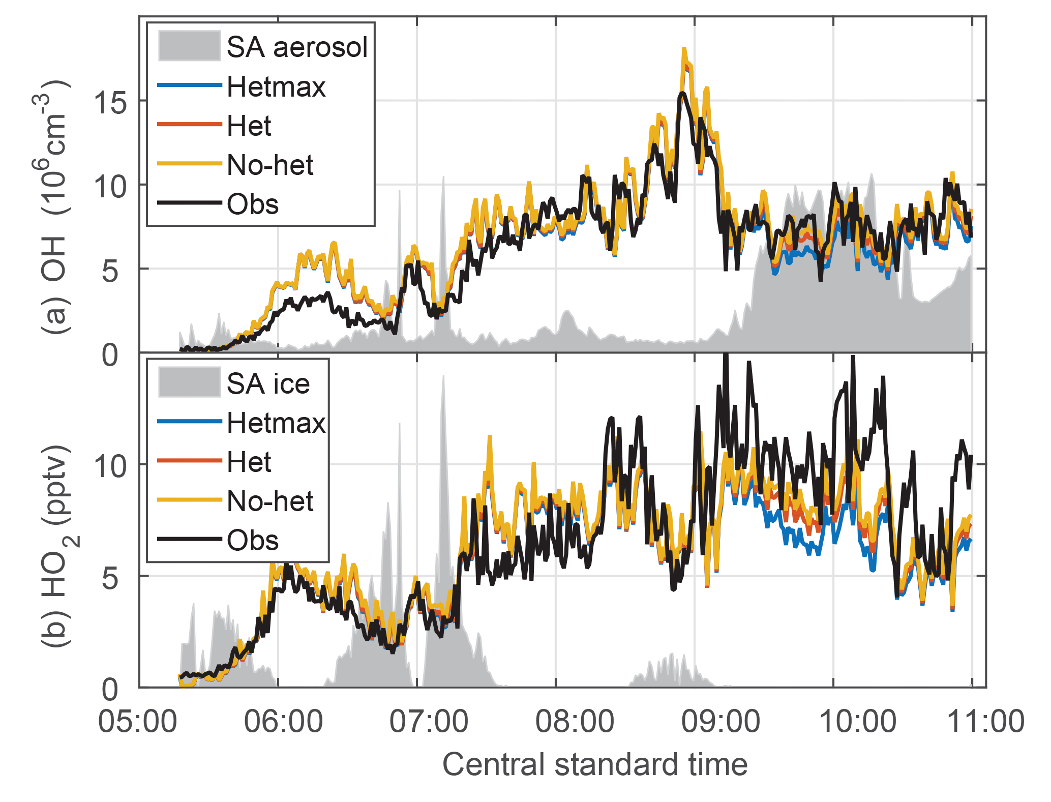
Figure 8Evolution of OH (a) and HO2 (b) downwind of a MCS. The het and hetmax models are essentially identical to the no-het model for this flight except in heavy aerosol amounts from 9:00 to 11:00 CST. The gray shading is scaled aerosol surface area (a) and is scaled ice surface area (b).
The quasi-Lagrangian tracking of convective outflow on 21 June provided an opportunity to test the photochemical evolution of OH and HO2 on the morning of 21 June. The flight legs perpendicular to the wind were approximately advected downwind. Initially, observed and modeled OH and HO2 were close to 0 (Fig. 8). However, both modeled OH and HO2 soon grew to exceed measured OH and HO2 by about 20 %–50 % until about 08:00 CST. For the remainder of the flight, observed and modeled OH are in substantial agreement for all three models, which are essentially identical except between 09:30 and 11:00 CST when the aerosol surface area per cm−3 of air was the greatest. For HO2, observed HO2 exceeds modeled by a factor of ∼1.5 after 09:00 CST. In this time period, the observations agree best with the no-het and het models. Thus, the basic observed behavior of OH and HO2 is captured by the no-het and het models although there is quantitative disagreement between the model and observations of OH and HO2 for local solar time between 05:45 and 08:15 CST and of HO2 after 09:00 CST.
Even though more than half of the first three legs were in an ice cloud, the scaled surface area for aerosol particles (Fig. 8a) and ice (Fig. 8b) does not correlate with the differences between observed and modeled OH and HO2.
As a test of the photochemistry, OH can be calculated from the observed decay of OH reactants. Nault et al. (2016) showed that the observed decay of ethane, ethyne, and toluene was consistent with an average observed OH of 9.5×106 cm−3 for times from 07:35 to 09:50 CST. An ATHOS recalibration since the publication of Nault et al. (2016) brings the mean observed number for this time interval down to 8.8×106 cm−3. This recalibration was needed to account for the window absorption of calibrated 185 nm radiation that was neglected in the initial DC3 calibration. This median revised observed OH concentration is consistent with the mean modeled OH concentration of 9.6×106 cm−3. These results agree well within uncertainties and support the observed OH.
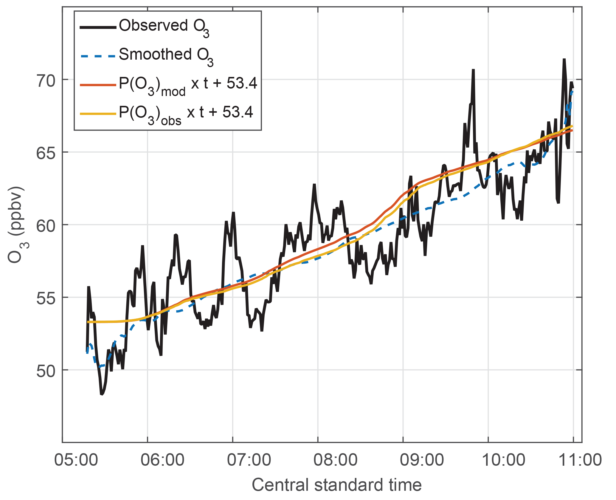
Figure 9The O3 trend in MCS outflow. Observed O3 – 1 min data (black line) and smoothed data (dashed blue line, 180 min filter) – shows variability along the legs set perpendicular to the air flow and also shows the O3 trend with time. The calculated O3 uses the accumulated calculated O3 production rates (P(O3) × time) for observed (yellow) and modeled HO2 (red) and adds those values to an initial value of 53.4 ppbv to show the calculated O3 trend.
Another good test of the photochemistry is a comparison between the observed O3 change and the accumulated calculated O3 production rate (Fig. 9). The O3 change is actually slightly larger than the observed O3 because some of the new O3 is partitioned into NO2, so that the quantity of interest is the change in O3 plus the change in NO2. The ozone production rate, P(O3), can be calculated with Eq. (3).
k is a reaction rate coefficient and L(O3) is the loss term for ozone. In this case, the loss term was only a few tenths ppbv h−1 (Fig. S9) and can be neglected. These rates are calculated in ppbv min−1 and then accumulated at times from 05:45 to 11:15 CST, in order to match the time period over which the DC-8 was sampling the MCS plume. This accumulated ozone production was calculated for the observed HO2 plus modeled RO2 and for the modeled HO2 plus modeled RO2. Modeled RO2 is primarily CH3O2 and CH3CH2O2 and its mixing ratio is half the HO2 mixing ratio above 5 km. HO2 accounts for a little more than half the total O3 production. In order to compare the observed O3 change to that accumulated from calculated O3 production, an ozone offset of 53.4 ppbv was added to the accumulated O3 production at 06:00 CST, which is when the ozone production commenced.
Ozone varied by 5–7 ppbv over the legs and was higher on one end of the leg than the other. These variations are smoothed using a 180 min filter. During the 5 h from 06:00 to 11:00 CST, the observed O3 change was 14 ppbv, although 2 ppbv of that change were in the final few minutes of observation. For the same time period, the ozone production calculated from modeled HO2 and modeled RO2 was 13 ppbv, and the ozone production calculated from observed HO2 and modeled RO2 was 13 ppbv. These three methods for determining O3 production agree to well within their uncertainties and provide additional confirmation of the observed and modeled HO2 and the modeled RO2.
These comparisons between median observed and modeled OH, HO2, and OH reactivity display an agreement that is generally within the combined uncertainties of the observations and model. This agreement within uncertainties generally holds in scatter plots and associated statistics and as a function of altitude, JO(1D), NO, O3, and the modeled OH reactivity. It also holds for the wide range of environments encountered during DC3, which includes different altitudes, cloudiness, and sunlight over roughly one-third of the continental United States.
A closer look at the figures shows seemingly random differences between observed and modeled OH and HO2. While most observed and modeled OH, HO2, and OH reactivity 1 min data are within the combined uncertainties (1σ confidence) of each other (57 %), there are sometimes persistent unexplained differences (Fig. S1). An example is from the 21 June flight over Missouri and Illinois (Fig. 8). For both OH and HO2, there are times when the modeled OH and HO2 are higher than the measurements, lower than the measurements, and equal to the measurements. At the same time, the measured OH reactivity is sometimes greater than the modeled OH reactivity and sometimes equal to it. These types of discrepancies are proving to be hard to resolve. A simple correlation analysis found no strong correlation between the observed-to-modeled ratio or difference and any model output variable. Employing more sophisticated methods in future work may be more productive.
4.1 Comparing DC3 to previous studies
All previous aircraft studies that included measurements of OH and HO2 have compared these observations to calculations from constrained photochemical box models. There is uncertainty in comparing the results from one study to another because often the instruments, their calibrations, and models are different or have evolved over time. Comparing results from very different environments amplifies this problem. As a result, the comparisons here are restricted to previous studies in air that was heavily influenced by convection.
NO, CO, O3, and JO(1D) from DC3 are remarkably similar to those observed in the Intercontinental Chemical Transport Experiment – North America Phase A (INTEX-A) in 2004 during flights over the central and eastern US (Ren et al., 2008) and to those observed from only 7 to 10 km for HOOVER 2 in summer 2007 during flights over central Europe (Regelin et al., 2013). As in DC3, observed and modeled OH agree to within uncertainties for INTEX-A and HOOVER 2 over their altitude ranges. On the other hand, observed and modeled HO2 agree to within uncertainties for DC3, HOOVER 2, and INTEX-A up to 8 km, but then observed HO2 grows to exceed modeled HO2 by a factor of 3 at 11 km for INTEX-A, in contrast to both DC3 and HOOVER 2 where observed and modeled HO2 agree to within the combined uncertainties.
One explanation for the HO2 discrepancy in INTEX-A could be the treatment of the HO2NO2 formation rate in the model. MCMv3.3.1 uses a reaction rate coefficient that takes the much lower low-temperature reaction rate coefficient of the laboratory study of Bacak et al. (2011) into account, while the Jet Propulsion Laboratory (JPL) evaluation (Burkholder et al., 2015) does not. For DC3, using the MCMv3.3.1 rate coefficient, observed-to-modeled OH and HO2 are 0.85–0.9 at altitudes above 10 km altitude, and modeled HO2NO2 is 1.9 times measured, but if the JPL recommended rate is used, then modeled OH and HO2 both increase by a factor of 1.5 at altitudes above 10 km, shifting the observed-to-modeled ratios to 1.3–1.4, while increasing modeled HO2NO2 to 5–10 times that observed (Fig. S10). The JPL-recommended reaction rate coefficient was used in the model for INTEX-A, which could explain some of the difference with DC3, except that the observed-to-modeled OH ratio should also be a factor of 3 for INTEX-A.
For DC3, observed and modeled HO2 appear to agree as a function of NO up to about 3 ppbv, which are the highest NO values encountered. For several previous ground-based studies, the observed HO2 was not obviously greater than the modeled HO2 until NO reached ∼2 ppbv or greater (Martinez et al., 2003; Ren et al., 2003; Shirley et al., 2006; Kanaya et al., 2007; Brune et al., 2016). For aircraft studies, in some cases, the observed HO2 did not obviously exceed the modeled HO2 until NO approached 2 ppbv (Baier et al., 2017), while in other studies, the obvious exceedance occurred when NO was only a few hundred pptv (Faloona et al., 2000; Ren et al., 2008). Olson et al. (2006) showed that the Faloona et al. (1999) results for the SUCCESS campaign (central US, 1996) could be explained by the averaging of sharp plumes containing high NO and depleted HO2 with the surrounding air. They showed that the SONEX (North Atlantic, 1997) results could be mostly explained by including all observed HOx precursors and updated kinetic rate coefficients and photolysis frequencies in the model. For INTEX-A (Ren et al., 2008), the enhanced NO is in the upper troposphere, where the observed-to-modeled HO2 reached a factor of 3. It is possible that the HO2 calibration was in error at low pressure (i.e., higher altitudes), although observed and modeled HO2 agree in the stratosphere. It is also possible that there were missing HO2 sources or outdated reaction rates in the model chemistry. We intend to re-examine INTEX-A and other previous NASA DC-8 missions that included ATHOS to see if an updated model can better simulate these HO2 observations.
The production rates of HOx (Fig. S11) and O3 (Fig. S9) are comparable to those found in previous studies (Ren et al., 2008; Olson et al., 2012). Modeled HOx production is dominated by O3 photolysis below 8 km, as has been previously observed (Regelin et al., 2013), but HCHO photolysis dominates above 10 km. HOx production by HONO photolysis essentially balances HOx loss by HONO formation. The calculated O3 production rates are also comparable to these other studies, which find production rates of a few ppbv h−1 in the PBL and above 10 km with a small loss at mid-altitude (Fig. S9). A spike in excess of 5 ppbv h−1 was found in a fire plume on 22 June (day of year 174), where abundances of both VOCs and NOx were enhanced.
4.2 Effects of heterogeneous chemistry on OH and HO2
These DC3 results indicate that a total uptake coefficient is much lower than 1 for aerosol. They also suggest that a total uptake coefficient of 0.2 is probably also too high because the model calculates HO2 values that are much lower than observed HO2 when the aerosol surface area per cm−3 of air was greater than 10−6 cm2 cm−3. In the DC3 environment, HOx has substantial gas-phase loss pathways, making it difficult for heterogeneous chemistry to be dominant when the model uses an uptake coefficient consistent with laboratory studies, except at the largest aerosol surface area per cm−3 of air. For the het case with a total uptake coefficient of 0.2, HOx loss including heterogeneous loss is 1.4 times the gas-phase-only loss when the aerosol surface area per cm−3 of air is cm2 cm−3, but grows to 1.5 at cm2 cm−3 and 2.5 for the few 1 min data points when it is greater than cm2 cm−3. This increase in HOx loss translates into decrease in the modeled HOx, with the decrease changing roughly as the square root of the increase in the HOx loss.
In DC3, the DC-8 spent hours flying in anvils of the cumulus clouds, which consisted of ice particles. DC3 provides evidence that the HO2 uptake on ice is small. These results are consistent with HO2 results over the western Pacific Ocean (Olson et al., 2004) but not with those over the northern Atlantic (Jeaglé et al., 2000). In Mauldin III et al. (1998), a large difference between the observed and modeled OH was found in clouds, but this difference may have been due to the lack of photolysis frequency measurements, which are crucial to test photochemistry in a cloudy environment. In DC3, the DC-8 spent essentially no time in liquid clouds, for which there is evidence of measurable HO2 uptake (Olson et al., 2006; Commane et al., 2010; Whalley et al., 2015). Thus, these DC3 results provide constraints of HO2 uptake on aerosol and ice particles, but not on liquid water particles.
In other cleaner environments or dirtier environments with a large amount of high aerosol surface area per cm−3 of air, heterogeneous chemistry can be a substantial fraction of the entire HOx loss and thus affect HO2 and OH abundances. Measuring OH and HO2 in these environments will provide a better test of the understanding of HO2 heterogeneous chemistry on aerosol particles than DC3 did.
The general agreement between the observed and modeled OH and HO2 for the complex DC3 environment is encouraging. It suggests that a photochemical box model can simulate the observed OH and HO2 to well within combined uncertainties, if properly constrained with measurements of other chemical species, photolysis frequencies, and environmental conditions. On the other hand, it is difficult to explain the unexpected deviations between observed and modeled OH and HO2, such as is observed in Figs. 8 or S1. Neither heterogeneous chemistry nor organic peroxyl chemistry are able to explain these deviations.
There are other possible causes for these discrepancies. First, it can be difficult to maintain instrument calibrations for not only OH and HO2 but also for all the other measurements that were used to constrain the model to calculate OH and HO2. Second, the simultaneous measurements need to be properly conditioned so that they can be used as model constraints. This process includes filling in isolated missing values because, if this was not done, the constraining data set would be sparse. For DC3, using the merged data set with no interpolation is less than 10 % of the full data set, but the observed and modeled OH and HO2 have essentially the same relationships as with the interpolated data set (Table S21). Third, the model parameters, such as integration times and decay times, must be set up so that the model calculations represent the observations and their variations. Varying these times caused a range of modeled values that was far smaller than the large observed-to-modeled differences, as seen in Fig. S1. For DC3, the 1 min data are adequate for the timescale of variations for most cases, except in small fire plumes and some spikes in lightning NOx in the anvil. Fourth, multiple methods are needed to determine if differences between observations and model are significant. For DC3, the comparisons between observations and models are robust despite the method of comparison. Thus, none of these appear to be the cause of the unexplained deviations between observed and modeled OH and HO2. A more thorough model uncertainty and sensitivity analysis could unveil the cause.
Even with these observed-to-modeled discrepancies, the general agreement for observed and modeled OH and HO2 suggests that current photochemical models can simulate observed atmospheric oxidation processes even around clouds to within these combined uncertainties. Reducing these uncertainties will enable comparisons of observed and modeled OH, and HO2 to provide a more stringent test of the understanding of atmospheric oxidation chemistry and thus to lead to an improvement in that understanding.
The Matlab code used for the zero-dimensional photochemical box modeling with the MCMv3.3.1 mechanism can be downloaded from Wolfe (2017). The paper describing this model is Wolfe et al. (2016).
The merge file for the DC3 DC-8 data and the updated OH, HO2, and OH reactivity numbers can be accessed by DOI: https://doi.org/10.5067/Aircraft/DC3/DC8/Aerosol-TraceGas (Aknan and Chen, 2017).
The supplement related to this article is available online at: https://doi.org/10.5194/acp-18-14493-2018-supplement.
WHB, XR, LZ, JM, DOM, BEA, DRB, RCC, GSD, SRH, TFH, LGH, BAN, JP, IP, TBR, TS, AS, KU, AW, and PJW made the DC3 measurements that are critical for the modeling and comparison of modeled and measured OH and HO2 in this paper. WB performed the modeling, did the analysis, wrote the manuscript, and made edits provided by the co-authors before submitting the manuscript.
The authors declare that they have no conflict of interest.
The Deep Convective Clouds and Chemistry (DC3) experiment is sponsored by the
U.S. National Science Foundation (NSF), the National Aeronautics and Space
Administration (NASA), the National Oceanic and Atmospheric Administration
(NOAA), and the Deutsches Zentrum für Luft- und Raumfahrt (DLR). Data
provided by NCAR/EOL are supported by the National Science Foundation.
Acetone/propanal measurements aboard the DC-8 during DC3 were supported by
the Austrian Federal Ministry for Transport, Innovation, and Technology
(BMVIT) through the Austrian Space Applications Programme (ASAP) of the
Austrian Research Promotion Agency (FFG). Support for ATHOS and OHR
measurements aboard the NASA DC-8 during DC3 comes from NASA grant
NNX12AB84G. We thank NASA management, pilots, and operations personnel for
the opportunity to gather these observations; the people of Salina, KS, for
hosting us and providing excellent facilities; Glenn Wolfe for his publicly
available F0AM model framework; and the University of Leeds for the publicly
available MCMv3.3.1 photochemical model. We also thank Joel Thornton for his
insights into HO2 heterogeneous chemistry, and Paul Lawson, Paul
Wennberg, John Crounse, and Jason. St. Clair
for the use of their
measurements.
Edited by: Dwayne Heard
Reviewed by: two anonymous referees
Aknan, A. and Chen, G.: NASA LaRC Airborne Science Data for Atmospheric Composition – DC3, https://doi.org/10.5067/Aircraft/DC3/DC8/Aerosol-TraceGas, 2017.
Apel, E. C., Olson, J. R., Crawford, J. H., Hornbrook, R. S., Hills, A. J., Cantrell, C. A., Emmons, L. K., Knapp, D. J., Hall, S., Mauldin III, R. L., Weinheimer, A. J., Fried, A., Blake, D. R., Crounse, J. D., Clair, J. M. St., Wennberg, P. O., Diskin, G. S., Fuelberg, H. E., Wisthaler, A., Mikoviny, T., Brune, W., and Riemer, D. D.: Impact of the deep convection of isoprene and other reactive trace species on radicals and ozone in the upper troposphere, Atmos. Chem. Phys., 12, 1135–1150, https://doi.org/10.5194/acp-12-1135-2012, 2012.
Apel, E. C., Hornbrook, R. S., Hills, A. J., Blake, N. J., Barth, M. C., Weinheimer, A., Cantrell, C., Rutledge, S. A., Basarab, B., Crawford, J., Diskin, G., Homeyer, C. R., Campos, T., Flocke, F., Fried, A., Blake, D. R., Brune, W., Pollack, I., Peischl, J. Ryerson, T., Wennberg, P. O., Crounse, J. D., Wisthaler, A., Mikoviny, T., Huey, G., Heikes, B., O'Sullivan, D., and Riemer, D. D.: Upper tropospheric ozone production from lightning NOx-impacted convection: Smoke ingestion case study from the DC3 campaign. J. Geophys. Res. Atmos., 120, 2505–2523, 2015.
Assaf, E., Sheps, L., Whalley, L., Heard, D., Tomas, A., Schoemaecker, C., and Fittschen, C.: The Reaction between CH3O2 and OH Radicals: Product Yields and Atmospheric Implications, Environ. Sci. Technol., 51, 2170–2177, https://doi.org/10.1021/acs.est.6b06265, 2017.
Bacak, A., Cooke, M. C., Bardwell, M. W., McGillen, M. R., Archibald, A. T., Huey, L. G., Tanner, D., Utembe, S. R., Jenkin, M. E., Derwent, R. G., Shallcross, D. E., and Percival, C. .: Kinetics of the HO2 + NO2 Reaction: On the Impact of New Gas-Phase Kinetic Data for the Formation of HO2NO2 on HOx, NOx and HO2NO2 Levels in the Troposphere, Atmos. Environ., 45, 6414–6422, 2011.
Baier, B. C., Brune, W. H., Miller, D. O., Blake, D., Long, R., Wisthaler, A., Cantrell, C., Fried, A., Heikes, B., Brown, S., McDuffie, E., Flocke, F., Apel, E., Kaser, L., and Weinheimer, A.: Higher measured than modeled ozone production at increased NOx levels in the Colorado Front Range, Atmos. Chem. Phys., 17, 11273–11292, https://doi.org/10.5194/acp-17-11273-2017, 2017.
Barth, M. C., Cantrell, C. A., Brune, W. H., Rutledge, S. A., Crawford, J. H., Huntrieser, H., Carey, L. D., MacGorman, D., Weisman, M., Pickering, K. E., Bruning, E., Anderson, B., Apel, E., Biggerstaff, M., Campos, T., Campuzano-Jost, P. Cohen, R., Crounse, J., Day, D. A., Diskin, G., Flocke, F., Fried, A., Garland, C., Heikes, B., Honomichl, S., Hornbrook, R., Huey, L. G., Jimenez, J. L., Lang, T., Lichtenstern, M., Mikoviny, T., Nault, B., O'Sullivan, D., Pan, L. L., Peischl, J., Pollack, I., Richter, D., Riemer, D., Ryerson, T., Schlager, H., St Clair, J., Walega, J., Weibring, P., Weinheimer, A., Wennberg, P., Wisthaler, A., Wooldridge, P. J., and Ziegler, C.: The Deep Convective Clouds and Chemsitry (DC3) Field Campaign, B. Am. Meteorol. Soc., 96, 1281–1309, 2015.
Barth, M. C., Bela, M. M., Fried, A., Wennberg, P. O., Crounse, J. D., St Clair, J. M., Blake, N. J., Blake, D. R., Homeyer, C. R., Brune, W. H., Zhang, L., Mao, J., Ren, X., Ryerson, T. B., Pollack, I. B., Peischl, J., Cohen, R. C., Nault, B. A., Huey, L. G., Liu, X., and Cantrell, C. A.: Convective transport and scavenging of peroxides by thunderstorms observed over the central US during DC3, J. Geophys. Res.-Atmos., 121, 4272–4295, 2016.
Bernt, T., Scholz, W., Mentler, B., Fischer, L., Herrmann, H., Kumala, M., and Hansel, A.: Accretion Product Formation from Self- and Cross-Reactions of RO2 Radicals in the Atmosphere, Angew. Chem. Int. Edit., 57, 3820–3824, https://doi.org/10.1002/anie.201710989, 2018.
Brune, W. H., Baier, B. C., Thomas, J., Ren, X., Cohen, R. C., Pusede, S. E., Browne, E. C., Goldstein, A. H., Gentner, D.R., Keutsch, F. N., Thornton, J. A., Harrold, S., Lopez-Hilfiker, F. D., and Wennberg, P. O.:, Ozone production chemistry in the presence of urban plumes, Faraday Discuss., 189, 169–189, 2016.
Burkholder, J. B., Sander, S. P., Abbatt, J., Barker, J. R., Huie, R. E., Kolb, C. E., Kurylo, M. J., Orkin, V. L., Wilmouth, D. M., and Wine, P. H.: Chemical Kinetics and Photochemical Data for Use in Atmospheric Studies, Evaluation No. 18, JPL Publication 15–10, Jet Propulsion Laboratory, Pasadena, https://doi.org/10.13140/RG.2.1.2504.2806, 2015.
Cazorla, M., Wolfe, G. M., Bailey, S. A., Swanson, A. K., Arkinson, H. L., and Hanisco, T. F.: A new airborne laser-induced fluorescence instrument for in situ detection of formaldehyde throughout the troposphere and lower stratosphere, Atmos. Meas. Tech., 8, 541–552, https://doi.org/10.5194/amt-8-541-2015, 2015.
Chatfield, R. B. and Crutzen, P. J.: Sulfur dioxide in remote oceanic air: Cloud transport of reactive precursors, J. Geophys. Res., 89, 7111–7132, https://doi.org/10.1029/JD089iD05p07111, 1984.
Chen, S., Brune, W. H., Oluwole, O. O., Kolb, C. E., Bacon, F., Li, G. Y., and Rabitz, H.: Global Sensitivity Analysis of the Regional Atmospheric Chemical Mechanism: An Application of Random Sampling-High Dimensional Model Representation to Urban Oxidation Chemistry, Environ. Sci. Technol., 46, 11162–11170, https://doi.org/10.1021/es301565w, 2012.
Christian, K. E., Brune, W. H., and Mao, J.: Global sensitivity analysis of the GEOS-Chem chemical transport model: ozone and hydrogen oxides during ARCTAS (2008), Atmos. Chem. Phys., 17, 3769–3784, https://doi.org/10.5194/acp-17-3769-2017, 2017.
Colman, J. J., Swanson, A. J., Meinardi, S., Sive, B. C., Blake, D. R., and Rowland, F. S.: Description of the Analysis of a Wide Range of Volatile Organic Compounds in Whole Air Samples Collected during PEM-Tropics A and B, Anal. Chem., 73, 3723–3731, 2001.
Commane, R., Floquet, C. F. A., Ingham, T., Stone, D., Evans, M. J., and Heard, D. E.: Observations of OH and HO2 radicals over West Africa, Atmos. Chem. Phys., 10, 8783–8801, https://doi.org/10.5194/acp-10-8783-2010, 2010.
Crounse, J. D., McKinney, K. A., Kwan, A. J., and Wennberg, P. O.: Measurement of gas-phase hydroperoxides by chemical ionization mass spectrometry, Anal. Chem., 78, 6726–6732, 2006.
Day, D. A., Woolridge, P. J., Dillon, M. B., Thornton, J. A., and Cohen, R. C.: A thermal dissociation laser-induced fluorescence instrument for in situ detection of NO2, peroxy nitrates, alkyl nitrates, and HNO3, J. Geophys. Res., 107, 4046–4053, 2002.
Faloona, I., Tan, D., Brune, W., Jaegle, L., Jacob, D., Kondo, Y., Koike, M., Chatfield, M., Pueschel, R., Ferry, G., Sachse, G., Vay, S., Anderson, B., Hannon, J., and Fuelberg, H.: Observations of HOx and its relationship with NOx in the upper troposphere during SONEX, J. Geophys. Res., 105, 3771–3783. 2000.
Faloona, I. C., Tan, D., Lesher, R. L., Hazen, N. L., Frame, C. L., Simpas, J. B., Harder, H., Martinez, M., Di Carlo, P., Ren, X. R., and Brune, W. H.: A laser-induced fluorescence instrument for detecting tropospheric OH and HO2: Characteristics and calibration, J. Atmos. Chem., 47, 139–167, 2004.
Fuchs, H., Bohn, B., Hofzumahaus, A., Holland, F., Lu, K. D., Nehr, S., Rohrer, F., and Wahner, A.: Detection of HO2 by laser-induced fluorescence: calibration and interferences from RO2 radicals, Atmos. Meas. Tech., 4, 1209–1225, https://doi.org/10.5194/amt-4-1209-2011, 2011.
Fuchs, H., Novelli, A., Rolletter, M., Hofzumahaus, A., Pfannerstill, E. Y., Kessel, S., Edtbauer, A., Williams, J., Michoud, V., Dusanter, S., Locoge, N., Zannoni, N., Gros, V., Truong, F., Sarda-Esteve, R., Cryer, D. R., Brumby, C. A., Whalley, L. K., Stone, D., Seakins, P. W., Heard, D. E., Schoemaecker, C., Blocquet, M., Coudert, S., Batut, S., Fittschen, C., Thames, A. B., Brune, W. H., Ernest, C., Harder, H., Muller, J. B. A., Elste, T., Kubistin, D., Andres, S., Bohn, B., Hohaus, T., Holland, F., Li, X., Rohrer, F., Kiendler-Scharr, A., Tillmann, R., Wegener, R., Yu, Z., Zou, Q., and Wahner, A.: Comparison of OH reactivity measurements in the atmospheric simulation chamber SAPHIR, Atmos. Meas. Tech., 10, 4023–4053, https://doi.org/10.5194/amt-10-4023-2017, 2017.
Hard, T. M., O'Brian, R. J., Chan, C. Y., and Mehrabzadeh, A. A.: Tropospheric free radical determination by FAGE, Environ. Sci. Technol., 18, 768–777, 1984.
Huey, L. G.: Measurement of trace atmospheric species by chemical ionization mass spectrometry: Speciation of reactive nitrogen and future directions, Mass Spectrom. Rev., 26, 166–184, 2007.
Jacob, D. J.: Heterogeneous chemistry and tropospheric ozone, Atmos. Environ., 34, 2131–2159, 2007.
Jaeglé, L., Jacob, D.J., Wennberg, P. O., Spivakowsky, C. M., Hanisco, T. F., Lanzendorf, E. J., Hintsa, E. J., Fahey, D. W., Keim, E. R., Proffitt, M. H., Atlas, E. L., Flocke, F., Schauffler, S., McElroy, C. T., Midwinter, C., Pfister, L., and Wilson, J. C.: Observed OH and HO2 in the upper troposphere suggest a major source from convective injection of peroxides, Geophys. Res. Lett., 24, 3181–3184, https://doi.org/10.1029/97GL03004, 1997.
Jaeglé, L., Jacob, D., Brune, W., Faloona, I., Tan, D., Heikes, B., Kondo, Y., Sachse, G., Anderson, B., Gregory, G., Singh, H., Pueschel, R., Ferry, G., Blake, D., and Shetter, R.: Photochemistry of HOx in the upper troposphere at northern latitudes, J. Geophys. Res., 105, 3877–3892, 2000.
Jenkin, M. E., Saunders, S. M., Wagner, V., and Pilling, M. J.: Protocol for the development of the Master Chemical Mechanism, MCM v3 (Part B): tropospheric degradation of aromatic volatile organic compounds, Atmos. Chem. Phys., 3, 181–193, https://doi.org/10.5194/acp-3-181-2003, 2003.
Kanaya, Y., Cao, R., Akimoto, H., Fukuda, M., Komazaki, Y., Yokouchi, Y., Koike, M., Tanimoto, H., Takegawa N., and Kondo, Y.: Urban photochemistry in central Tokyo: 1. Observed and modeled OH and HO2 radical concentrations during the winter and summer of 2004, J. Geophys. Res., 112, D21312, https://doi.org/10.1029/2007jd008670, 2007.
Kovacs, T. and Brune, W.: Total OH Loss Rate Measurement, J. Atmos. Chem., 39, 105–122, 2001.
Kubistin, D., Harder, H., Martinez, M., Rudolf, M., Sander, R., Bozem, H., Eerdekens, G., Fischer, H., Gurk, C., Klüpfel, T., Königstedt, R., Parchatka, U., Schiller, C. L., Stickler, A., Taraborrelli, D., Williams, J., and Lelieveld, J.: Hydroxyl radicals in the tropical troposphere over the Suriname rainforest: comparison of measurements with the box model MECCA, Atmos. Chem. Phys., 10, 9705–9728, https://doi.org/10.5194/acp-10-9705-2010, 2010.
Lakey, P. S. J, George, I. J., Baeza-Romero, M. T., Whalley, L. K., and Heard, D. E.: Organics Substantially Reduce HO2 Uptake onto Aerosols Containing Transition Metal ions, J. Phys. Chem. A, 120, 1421–1430, https://doi.org/10.1021/acs.jpca.5b06316, 2015.
Lakey, P. S. J., Berkemeier, T., Krapf, M., Dommen, J., Steimer, S. S., Whalley, L. K., Ingham, T., Baeza-Romero, M. T., Pöschl, U., Shiraiwa, M., Ammann, M., and Heard, D. E.: The effect of viscosity and diffusion on the HO2 uptake by sucrose and secondary organic aerosol particles, Atmos. Chem. Phys., 16, 13035–13047, https://doi.org/10.5194/acp-16-13035-2016, 2016.
Logan, J. A., Prather, M. J., Wofsy, S. C., and McElroy: M. B., Tropospheric chemistry: A global perspective, J. Geophys. Res., 86, 7210–7254, 1981.
Mao, J., Ren, X., Brune, W. H., Olson, J. R., Crawford, J. H., Fried, A., Huey, L. G., Cohen, R. C., Heikes, B., Singh, H. B., Blake, D. R., Sachse, G. W., Diskin, G. S., Hall, S. R., and Shetter, R. E.: Airborne measurement of OH reactivity during INTEX-B, Atmos. Chem. Phys., 9, 163–173, https://doi.org/10.5194/acp-9-163-2009, 2009.
Mao, J., Jacob, D. J., Evans, M. J., Olson, J. R., Ren, X., Brune, W. H., Clair, J. M. St., Crounse, J. D., Spencer, K. M., Beaver, M. R., Wennberg, P. O., Cubison, M. J., Jimenez, J. L., Fried, A., Weibring, P., Walega, J. G., Hall, S. R., Weinheimer, A. J., Cohen, R. C., Chen, G., Crawford, J. H., McNaughton, C., Clarke, A. D., Jaeglé, L., Fisher, J. A., Yantosca, R. M., Le Sager, P., and Carouge, C.: Chemistry of hydrogen oxide radicals (HOx) in the Arctic troposphere in spring, Atmos. Chem. Phys., 10, 5823–5838, https://doi.org/10.5194/acp-10-5823-2010, 2010.
Mao, J., Ren, X., Zhang, L., Van Duin, D. M., Cohen, R. C., Park, J.-H., Goldstein, A. H., Paulot, F., Beaver, M. R., Crounse, J. D., Wennberg, P. O., DiGangi, J. P., Henry, S. B., Keutsch, F. N., Park, C., Schade, G. W., Wolfe, G. M., Thornton, J. A., and Brune, W. H.: Insights into hydroxyl measurements and atmospheric oxidation in a California forest, Atmos. Chem. Phys., 12, 8009–8020, https://doi.org/10.5194/acp-12-8009-2012, 2012.
Martinez, M, Harder, H., Kovacs, T. A., Simpas, J. B., Bassis, J., Lesher, R., Brune, W. H., Frost, G. J., Williams, E. J., Stroud, C. A., Jobson, B. T., Roberts, J. M., Hall, S. R., Shetter, R. E., Wert, B., Fried, A., Alicke, B., Stutz, J., Young, V. L., White, A. B., and Zamora, R. J.: OH and HO2 concentrations, sources, and loss rates during the Southern Oxidants Study in Nashville, Tennessee, summer 1999, J. Geophys. Res.-Atmos., 108, 4617, https://doi.org/10.1029/2003JD003551, 2003.
Mauldin III, R. L., Tanner, D. J., Frost, G. J., Chen, G., Prevot, A. S. H., Davis, D. D., and Eisele, F. L.: OH measurements during ACE-1: observations and model comparisons, J. Geophys. Res.-Atmos., 103, 16713–16729, 1998.
Mielke, L. H., Erickson, D. E., McLuckey, S. A., Müller, M., Wisthaler, A., Hansel, A., and Shepson, P. B.: Development of a Proton-Transfer Reaction-Linear Ion Trap Mass Spectrometer for Quantitative Determination of Volatile Organic Compounds, Anal. Chem., 80, 8171–8177, https://doi.org/10.1021/ac801328d, 2008.
Nault, B. A., Garland, C., Wooldridge, P. J., Brune, W. H., Campuzano-Jost, J., Crounse, J. D., Day, D. A., Dibb, J., Hall, S. R., Huey, L. G., Jimenez, J. L., Liu, X. X., Mao, J. Q., Mikoviny, T., Peischl, J., Pollack, I. B., Ren, X. R., Ryerson, T. B., Scheuer, E., Ullmann, K., and Wennberg, P. O., Wisthaler, A., Zhang, L., and Cohen, R.C.: Observational Constraints on the Oxidation of NOx in the Upper Troposphere, J. Phys. Chem. A, 120, 1468–1478, 2016.
Nault, B. A., Laughner, J. L., Wooldridge, P. J., Crounse, J. D., Dibb, J., Diskin, G., and Cohen, R. C.: Lightning NOx emissions: reconciling measured and modeled estimates with updated NOx chemistry, Geophys. Res. Lett., 44, 9479–9488, https://doi.org/10.1002/2017GL074436, 2017.
Olson, J. R., Crawford, J. H., Chen, G., Fried, A., Evans, M., Jordan, C. E., Sandholm, S. T., Davis, D. D., Anderson, B. E., Avery, M. A., Barrick, J. D., Blake, D. R., Brune, W. H., Eisele, F. L., Flocke, F., Harder, H., Jacob, D. J., Kondo, Y., Lefer, B. L., Martinez M., Mauldin, R. L., Sachse, G. W., Shetter, R. E., Singh, H. B., Talbot, R. W., and Tan D.:, Testing fast photochemical theory during TRACE-P based on measurements of OH, HO2, and CH2O, J. Geophys. Res.-Atmos., 109, D15S10, https://doi.org/10.1029/2003JD004278, 2004.
Olson, J. R., Crawford, J. H., Chen, G., Brune, W. H., Faloona, I. C., Tan, D., Harder, H., and Martinez, M.: A reevaluation of airborne HOx observations from NASA field campaigns, J. Geophys. Res.-Atmos., 111, D10301, https://doi.org/10.1029/2005JD006617, 2006.
Olson, J. R., Crawford, J. H., Brune, W., Mao, J., Ren, X., Fried, A., Anderson, B., Apel, E., Beaver, M., Blake, D., Chen, G., Crounse, J., Dibb, J., Diskin, G., Hall, S. R., Huey, L. G., Knapp, D., Richter, D., Riemer, D., Clair, J. St., Ullmann, K., Walega, J., Weibring, P., Weinheimer, A., Wennberg, P., and Wisthaler, A.: An analysis of fast photochemistry over high northern latitudes during spring and summer using in-situ observations from ARCTAS and TOPSE, Atmos. Chem. Phys., 12, 6799–6825, https://doi.org/10.5194/acp-12-6799-2012, 2012.
Pickering, K. E., Thompson, A. M., Dickerson, R. R., Luke, W. T., McNamara, D. P., Greenberg, J. P., and Zimmerman, P. R.: Model calculations of tropospheric ozone production potential following observed convective events, J. Geophys. Res.-Atmos., 95, 14049–14062, https://doi.org/10.1029/JD095iD09p14049, 1990.
Pollack, I. B., Lerner, B. M., and Ryerson, T. B.: Evaluation of ultraviolet light-emitting diodes for detection of atmospheric NO2 by photolysis-chemiluminescence, J. Atmos. Chem., 65, 111–125, https://doi.org/10.1007/s10874-011-9184-3, 2011.
Pollack, I. B., Homeyer, C. R., Ryerson, T. B., Aikin, K. C., Peichl, J., Apel, E. C., Campos, T., Flocke, F., Hornbrook, R. S., Knapp, D. J., Montzka, D. D., Weinheimer, A. J., Riemer, D., Diskin, G., Sachse, G., Mikoviny, T., Wisthaler, A., Bruning, E., MacGorman, D., Cummings, K. A., Pickering, K. E., Huntrieser, H., Lichtenstern, M., Schlager, H., and Barth, M. C.: Airborne quantification of upper tropospheric NOx production from lightning in deep convective storms over the United States Great Plains, J. Geophys. Res.-Atmos., 121, 2002–2028, https://doi.org/10.1002/2015JD023941, 2016.
Ravetta, F., Jacob, D. J., Brune, W. H., Tan, D., Faloona, I. F., Heikes, B. J., Anderson, B., Blake, D. R., Gregory, G. L., Sachse, G. W., Sandholm, S. T., Shetter, R. E., Singh, H. E., and Talbot, R. W.: Experimental evidence for the importance of convected methylhydroperoxide as a source of hydrogen oxide (HOx) radicals in the tropical upper troposphere, J. Geophys. Res.-Atmos., 106, 32709–32716, 2001.
Regelin, E., Harder, H., Martinez, M., Kubistin, D., Tatum Ernest, C., Bozem, H., Klippel, T., Hosaynali-Beygi, Z., Fischer, H., Sander, R., Jöckel, P., Königstedt, R., and Lelieveld, J.: HOx measurements in the summertime upper troposphere over Europe: a comparison of observations to a box model and a 3-D model, Atmos. Chem. Phys., 13, 10703–10720, https://doi.org/10.5194/acp-13-10703-2013, 2013.
Ren, X. R., Harder, H., Martinez, M., Lesher, R. L., Oliger, A., Shirley, T., Adams, J., Simpas, J. B., andBrune, W.H.: HOx concentrations and OH reactivity observations in New York City during PMTACS-NY2001, Atmos. Environ., 37, 3627–3637, 2003.
Ren, X. R., Olson, J. R., Crawford, J. H., Brune, W. H., Mao, J. Q., Long, R. B., Chen, Z., Chen, G., Avery, M. A., Sachse, G. W., Barrick, J. D., Diskin, G. S., Huey, L. G., Fried, A., Cohen, R. C., Heikes, B., Wennberg, P. O., Singh, H. B., Blake, D. R., and Shetter, R. E.: HOx chemistry during INTEX-A 2004: Observation, model calculation, and comparison with previous studies, J. Geophys. Res.-Atmos., 113, D05319, https://doi.org/10.1029/2007JD009166, 2008.
Ren, X., Mao, J., Brune, W. H., Cantrell, C. A., Mauldin III, R. L., Hornbrook, R. S., Kosciuch, E., Olson, J. R., Crawford, J. H., Chen, G., and Singh, H. B.: Airborne intercomparison of HOx measurements using laser-induced fluorescence and chemical ionization mass spectrometry during ARCTAS, Atmos. Meas. Tech., 5, 2025–2037, https://doi.org/10.5194/amt-5-2025-2012, 2012.
Ridley, B. A., Dye, J., Walega, J. G., Zheng, J., Grahek, F. E., and Rison, W.: On the production of active nitrogen by thunderstorms over New Mexico, J. Geophys. Res.-Atmos., 101, 20985–21005, https://doi.org/10.1029/96JD01706, 1996.
Ryerson, T. B., Williams, E. J., and Fehsenfeld, F. C.: An efficient photolysis system for fast-response NO2 measurements, J. Geophys. Res., 105, 26447–26461, 2000.
Sachse, G. W., Collins, J. E., Hill, G. F., Wade, L. O., Burney, L. G., and Ritter, J. A.: Airborne tunable diode-laser sensor for high-precision concentration and flux measurements of carbon-monoxide and methane, Proc. SPIE, 1433, 157–166, 1991.
Saunders, S. M., Jenkin, M. E., Derwent, R. G., and Pilling, M. J.: Protocol for the development of the Master Chemical Mechanism, MCM v3 (Part A): tropospheric degradation of non-aromatic volatile organic compounds, Atmos. Chem. Phys., 3, 161–180, https://doi.org/10.5194/acp-3-161-2003, 2003.
Shirley, T. R., Brune, W. H., Ren, X., Mao, J., Lesher, R., Cardenas, B., Volkamer, R., Molina, L. T., Molina, M. J., Lamb, B., Velasco, E., Jobson, T., and Alexander, M.: Atmospheric oxidation in the Mexico City Metropolitan Area (MCMA) during April 2003, Atmos. Chem. Phys., 6, 2753–2765, https://doi.org/10.5194/acp-6-2753-2006, 2006.
Schumann, U. and Huntrieser, H.: The global lightning-induced nitrogen oxides source, Atmos. Chem. Phys., 7, 3823–3907, https://doi.org/10.5194/acp-7-3823-2007, 2007.
Stone, D., Evans, M. J., Commane, R., Ingham, T., Floquet, C. F. A., McQuaid, J. B., Brookes, D. M., Monks, P. S., Purvis, R., Hamilton, J. F., Hopkins, J., Lee, J., Lewis, A. C., Stewart, D., Murphy, J. G., Mills, G., Oram, D., Reeves, C. E., and Heard, D. E.: HOx observations over West Africa during AMMA: impact of isoprene and NOx, Atmos. Chem. Phys., 10, 9415–9429, https://doi.org/10.5194/acp-10-9415-2010, 2010.
Stone, D., Whalley, L. K., and Heard, D. E.: Tropospheric OH and HO2 radicals: field measurements and model comparisons, Chem. Soc. Rev., 41, 6348–6404, 2012.
Tan, D., Faloona, I., Simpas, J. B., Brune, W., Olson, J., Crawford, J., Sandholm, S., Guan, H.-W., Vaughn, T., Mastromarino, J., Sachse, G., Vay, S., Podolske, J., Avery, M., Heikes, B., Snow, J., and Singh, H.: OH and HO2 in the remote tropical Pacific: results from PEM-Tropics B, J. Geophys. Res., 106, 32667–32681, 2001.
Tang, M. J., Cox, R. A., and Kalberer, M.: Compilation and evaluation of gas phase diffusion coefficients of reactive trace gases in the atmosphere: volume 1. Inorganic compounds, Atmos. Chem. Phys., 14, 9233–9247, https://doi.org/10.5194/acp-14-9233-2014, 2014.
Thompson, A. M. and Stewart, R. W.: Effect of chemical kinetics uncertainties on calculated constituents in a tropospheric photochemical model, J. Geophys. Res.-Atmos., 96, 13089–13108, https://doi.org/10.1029/91JD01056, 1991.
Thornton, J. A., Wooldridge, P. J., and Cohen, R. C.: Atmospheric NO2: In situ Laser-Induced Fluorescence Detection at Parts per Trillion Mixing Ratios, Anal. Chem., 72, 528–539, 2000.
Thornton, J. A., Jaeglé, L., and McNeill, V. F.: Assessing known pathways for HO2 loss in aqueous atmospheric aerosols: Regional and global impacts on tropospheric oxidants, J. Geophys. Res.-Atmos., 113, D05303, https://doi.org/10.1029/2007JD009236, 2008.
Vay, S. A., Anderson, B. E., Sachse, G. W., Collins Jr., J. E., Podolske, J. R., Twohy, C. W., Gandrud, B., Chan, K. R., Baughcum, S. L., and Wallio, H. A.: DC-8-based observations of aircraft CO, CH4, N2O, and H2O(g) emission indices during SUCCESS, Geophys. Res. Lett., 25, 1717–1720, 1998.
Wennberg, P. O., Hanisco, T. F., Jaegle, L., Jacob, D. J., Hintsa, E. J., Lanzendorf, E. J., Anderson, J. G., Gao, R.-S., Keim, E. R., Donnelly, S. G., Del Negro, L. A., Fahey, D. W., McKeen, S. A., Salawitch, R. J., Webster, C. R., May, R. D., Herman, R. L., Proffitt, M. H., Margitan, J. J., Atlas, E. L., Schauffler, S. M., Flocke, F., McElroy, C. T., and Bui, T. P.: Hydrogen radicals, nitrogen radicals, and the production of O3 in the upper troposphere, Science, 279, 49–53, 1998.
Whalley, L. K., Stone, D., George, I. J., Mertes, S., van Pinxteren, D., Tilgner, A., Herrmann, H., Evans, M. J., and Heard, D. E.: The influence of clouds on radical concentrations: observations and modelling studies of HOx during the Hill Cap Cloud Thuringia (HCCT) campaign in 2010, Atmos. Chem. Phys., 15, 3289–3301, https://doi.org/10.5194/acp-15-3289-2015, 2015.
Wolfe, G. M.: F0AM Box Model, available at: https://sites.google.com/site/wolfegm/models, 2017.
Wolfe, G. M., Marvin, M. R., Roberts, S. J., Travis, K. R., and Liao, J.: The Framework for 0-D Atmospheric Modeling (F0AM) v3.1, Geosci. Model Dev., 9, 3309–3319, https://doi.org/10.5194/gmd-9-3309-2016, 2016.
York, D., Evensen, N., Martinez, M., and Delgado, J.: Unified equations for the slope, intercept, and standard errors of the best straight line, Am. J. Phys., 72, 367–375, https://doi.org/10.1119/1.1632486, 2004.