the Creative Commons Attribution 4.0 License.
the Creative Commons Attribution 4.0 License.
 | 01 Oct 2018
Long-term measurements of volatile organic compounds highlight the importance of sesquiterpenes for the atmospheric chemistry of a boreal forest
Arnaud P. Praplan
Toni Tykkä
Ilona Ylivinkka
Ville Vakkari
Jaana Bäck
Tuukka Petäjä
Markku Kulmala
Hannele Hakola
The concentrations of terpenoids (isoprene; monoterpenes, MTs; and sesquiterpenes, SQTs) and oxygenated volatile organic compounds (OVOCs; i.e. aldehydes, alcohols, acetates and volatile organic acids, VOAs) were investigated during 2 years at a boreal forest site in Hyytiälä, Finland, using in situ gas chromatograph mass spectrometers (GC-MSs). Seasonal and diurnal variations of terpenoid and OVOC concentrations as well as their relationship with meteorological factors were studied.
Of the VOCs examined, C2–C7 unbranched VOAs showed the highest concentrations, mainly due to their low reactivity. Of the terpenoids, MTs showed the highest concentrations at the site, but seven different highly reactive SQTs were also detected. The monthly and daily mean concentrations of most terpenoids, aldehydes and VOAs were highly dependent on the temperature. The highest exponential correlation with temperature was found for a SQT (β-caryophyllene) in summer. The diurnal variations in the concentrations could be explained by sources, sinks and vertical mixing. The diurnal variations in MT concentrations were strongly affected by vertical mixing. Based on the temperature correlations and mixing layer height (MLH), simple proxies were developed for estimating the MT and SQT concentrations.
To estimate the importance of different compound groups and compounds in local atmospheric chemistry, reactivity with main oxidants (hydroxyl radical, OH; nitrate radical, NO3; and ozone, O3) and production rates of oxidation products (OxPRs) were calculated. The MTs dominated OH and NO3 radical chemistry, but the SQTs greatly impacted O3 chemistry, even though the concentrations of SQT were 30 times lower than the MT concentrations. SQTs were also the most important for the production of oxidation products. Since the SQTs show high secondary organic aerosol (SOA) yields, the results clearly indicate the importance of SQTs for local SOA production.
- Article
(8011 KB) -
Supplement
(1927 KB) - BibTeX
- EndNote


The boreal forest is one of the largest terrestrial biomes in the world, forming an almost continuous belt around the Northern Hemisphere. It is characterised by large volatile organic compound (VOC) emissions with strong seasonal variations (Sindelarova et al., 2014). The boreal zone is believed to be a major source of climate-relevant biogenic aerosol particles produced from the reaction products of primary emitted biogenic VOCs (BVOCs, Tunved et al., 2006). Isoprene, monoterpenes (MTs) and sesquiterpenes (SQTs) are the main reactive BVOCs emitted from the boreal forest (Guenther et al., 2012). They are known to influence particle formation and growth (e.g. Kulmala et al., 2013), the oxidation capacity of the atmosphere (Peräkylä et al., 2014), and chemical communication by plants and insects (Holopainen, 2004). Oxygenated VOCs (OVOCs) emitted from the vegetation include carbonyls, alcohols and volatile organic acids (VOAs), but their emissions are less studied and they are also produced in the atmosphere from the reactions of VOCs (Mellouki et al., 2015). Studies on total reactivity in the atmosphere of boreal forests have suggested the presence of highly reactive unmeasured BVOCs (Sinha et al., 2010; Nölscher et al., 2012; Praplan et al., 2018). In other vegetation zones, the fraction of unmeasured BVOCs has also been very high (up to 80 %; Yang et al., 2016). Therefore, better characterisation of BVOC emissions and concentrations in forested areas is needed.
Once emitted, BVOCs readily react with atmospheric oxidants, and the photochemical oxidation of even small organic compounds can lead to the formation of tens to hundreds of first-generation products, which then undergo further oxidation and transformation (Glasius and Goldstein, 2016). Thus, it will probably never be possible to identify all oxidation products (OxPRs) of all VOCs in the atmosphere. Therefore, detailed knowledge on the primary emitted compounds is crucial. The reaction rates, reaction paths and secondary organic aerosol (SOA) yields of the various terpenoids are very different (Lee et al., 2006; Ng et al., 2017), and compound-specific concentration data are essential to an understanding of biosphere–atmosphere interactions as well as local and regional atmospheric chemistry.
Proton-transfer-reaction mass spectrometers (PTR-MSs) are often used for measurements of fluxes or concentrations of MTs (Yuan et al., 2017) and there are already long data sets on ambient air concentrations of MTs measured by PTR-MSs even in boreal forest (Lappalainen et al., 2009; Kontkanen et al., 2016). PTR-MS measurements of SQT concentrations have often not been done, but there are some data available from the tropical forests (Kim et al., 2009, 2010; Jardine et al., 2011). However, PTR-MSs are not able to distinguish the various MTs or SQTs. Data on the concentrations of individual MTs measured by gas chromatograph mass spectrometers (GC-MSs) are scarce and often available only from short measurement campaigns (Kesselmeier et al., 2002; Hakola et al., 2003, 2009; Jones et al., 2011; Yassaa et al., 2012; Jardine et al., 2015; Yáñez-Serrano et al., 2018). Emissions of both MTs and SQTs have been studied in various vegetation zones (Guenther et al., 2012), but to our knowledge only three studies are available on the atmospheric concentrations of individual SQTs (Bouvier-Brown et al., 2009; Hakola et al., 2012; Yee et al., 2018). Bouvier-Brown et al. (2009) measured the ambient air concentrations of MTs and SQTs in a ponderosa pine forest in California from 20 August until 10 October in 2007 with an in situ GC-MS, and Hakola et al. (2012) measured MTs and SQTs in the air of a boreal forest in Finland in 2011. However, due to losses in the inlets and less sensitive instruments, both studies were missing β-caryophyllene, which is the main SQT known to be emitted by pine trees (Hakola et al., 2006). Yee et al. (2018) conducted SQT measurements in the central Amazon rainforest for over 4 months in 2014 and found 30 different SQTs. However, their site was located 2.5 km from the forest and they concluded that the most reactive compounds had already reacted away before arriving at the site. For example, they did not detect β-caryophyllene even though they were able to find many of its reaction products. Emission chamber measurements often suffer from losses of the most reactive SQTs on the chamber walls and inlet lines, and canopy-scale flux measurements are often not available due to the rapid reactions and low concentrations of SQTs. Therefore, ambient concentration data are clearly needed to constrain the emissions of SQTs (Duhl et al., 2008). We report here what we believe are the first quantitative measurements of the ambient concentrations of β-caryophyllene, the main SQT emitted by the boreal forest trees (Hakola et al., 2001, 2006).
Regarding OVOCs, studies of the emissions of small compounds (e.g. methanol, acetone, acetaldehyde, acetic acid) have been conducted (e.g. Aalto et al., 2014; Sindelarova et al., 2014). However, knowledge of the biogenic sources and concentrations of the larger volatile carbonyls, alcohols (C5–C10) and VOAs is very limited.
In this study, the ambient air measurements of individual BVOCs and OVOCs were conducted in 2015 and 2016 in a boreal forest at the Station for Measuring Ecosystem–Atmosphere Relations (SMEAR II) site in Hyytiälä with in situ GC-MSs. We experienced technical difficulties In the VOC measurements, and, even with the intensive campaign, our data do not cover the entire measuring period continuously. To parameterise the concentrations, understand their sources and fill the gaps in the data, we studied the dependence of the concentrations on environmental factors. Since temperature is the dominant factor controlling the emissions of these BVOCs from trees at Hyytiälä (e.g. Tarvainen et al., 2005; Hakola et al., 2006, 2017), the main focus was set on temperature dependence. Based on the temperature correlations, simplified proxies for estimating local concentrations were developed. To estimate the importance of the individual VOCs or VOC groups for the local atmospheric chemistry and SOA production, reactivities and the production rates of oxidation products were calculated.
2.1 Measurement site
The measurements were conducted in a boreal forest at SMEAR II in southern Finland. The SMEAR II station is a dedicated facility for studying the forest ecosystem–atmosphere relationships (Hari and Kulmala, 2005). The measurement station is located in Hyytiälä ( N, E; 181 m above sea level) in an approximately 55-year-old managed coniferous forest. The continuous measurements at the site include leaf-, stand- and ecosystem-scale measurements of greenhouse gases, pollutants (e.g. ozone, O3; sulfur dioxide, SO2; nitrogen oxide, NOx) and many different aerosol, vegetation and soil properties. In addition, a full suite of meteorological measurements was collected.
The vegetation nearest to the measurement container was a homogeneous Scots pine (Pinus sylvestris L.) forest (>60 %) where some birch (Betula sp.), poplar (Populus sp.) and Norway spruce (Picea abies) grow below the canopy. The canopy height is about 20 m with an average tree density of 1370 stems (diameter at breast height >5 cm) per hectare (Ilvesniemi et al., 2009). The understorey vegetation is comprised of various shrubs, grasses and moss species. The most common shrubs are cowberry (Vaccinium vitis-idaea L.) and bilberry (Vaccinium myrtillus L.), the most common mosses are Schreber's big red stem moss (Pleurozium schreberi (Brid.) Mitt.) and a dicranum moss (Dicranum Hedw. sp.), and the most common grasses are wavy hair-grass (Deschampsia flexuosa (L.) Trin.) and small cow-wheat (Melampyrum sylvaticum L.). Anthropogenic influence at the site is low. The largest nearby city is Tampere with 200 000 inhabitants. It is located 60 km to the southwest of the site.
2.2 Volatile organic compound measurements
Ambient air measurements of VOCs were conducted in 2011, 2015 and 2016. Data from 2011 were published earlier by Hakola et al. (2012). The concentrations were measured with three different in situ thermal-desorption gas chromatograph mass spectrometers (TD-GC-MSs), described hereafter as GC-MS1, GC-MS2 and GC-MS3. In 2015 and 2016 two different GC-MSs were used in parallel. The instruments were located in a container about 4 m outside the forest in a gravel-bedded clearing. In 2015 and 2016 samples for the GC-MSs were taken at a height of 1.5 m from an inlet reaching out approximately 30 cm from the container wall. In 2011 the GC-MS inlet was on the roof of a container at about 2.5 m.
The GC-MS1 was used for the measurements of isoprene and individual MTs in 2011 and May–July 2015. With the GC-MS1 air was drawn through a 3 m long stainless steel tube (1∕4 in. outer diameter, o.d.) at a flow rate of 1 L min−1. The tubes were heated to 120 ∘C to avoid losses of terpenoids. A stainless steel (grade 304 or 316) inlet line heated to 120 ∘C was used to destroy O3, and losses for SQTs and MTs are negligible. This method is described in detail by Hellén et al. (2012). Removal of O3 from the inlet flow before collection of the sample is essential for avoiding losses of the very O3-reactive compounds (e.g. β-caryophyllene). VOCs in a 30–50 mL min−1 subsample were collected in the cold trap of the thermal-desorption unit (ATD-400; PerkinElmer Inc., Waltham, MA, USA) packed with Tenax TA in 2011 and Tenax TA–Carbopack B in 2015 and analysed in situ with a GC (HP 5890; Agilent Technologies Inc., Santa Clara, CA, USA) with a DB-1 column (60 m; inner diameter, i.d., 0.25 mm; film thickness, 0.25 µm) and a mass-selective detector (HP 5972, Agilent Technologies). One 60 min sample was collected every second hour. The detection limits were below 1 ppt for all MTs. Measurements with the GC-MS1 were described in detail by Hakola et al. (2012). The system was calibrated using liquid standards in methanol solutions injected on Tenax TA and Carbopack B adsorbent tubes and analysed between the samples using the offline mode of the instrument. The stability of the MS was characterised using tetrachloromethane as an “internal standard”. The local concentration of tetrachloromethane in the ambient air was stable, and thus it was possible to detect sampling errors or shifts in calibration levels by measuring its concentration.
The GC-MS2 was used for the measurements of C5–C8 alcohols, C2–C7 VOAs and the MT sum in May–October 2015 and February–September 2016. Samples were taken every second hour. In the 3 m long fluorinated ethylene propylene (FEP) inlet (1∕8 in. i.d.), an inlet flow of 2.2 L min−1 was used to avoid losses of the compounds on the walls of the inlet tube. The samples were collected as subsamples from this ambient airflow into the cold trap (U-T17O3P-2S, Markes International Ltd, Llantrisant, Wales, UK) of the thermal-desorption unit (Unity 2 + Air Server 2, Markes International). The sampling time was 60 min and the sampling flow through the cold trap 30 mL min−1. Heated stainless steel tubing (1 m) was used for O3 removal (Hellén et al., 2012). Samples were analysed in situ with a GC (Agilent 7890A, Agilent Technologies) and a MS (Agilent 5975C, Agilent Technologies) connected to the thermal-desorption unit. The polyethylene glycol column used for separation was the 30 m DB-WAXetr (J&W 122-7332, Agilent Technologies) with an i.d. of 0.25 mm and a film thickness of 0.25 µm. The system was calibrated using liquid standards in Milli-Q water (VOAs) and methanol (other VOCs) injected into adsorbent tubes filled with Tenax TA (60∕80 mesh, Supelco Inc., Bellefonte, PA, USA) and Carbopack B (60∕80 mesh, Supelco Inc.) and analysed by the same method as samples. Liquid standards were injected into the clean nitrogen flow, which was flushed through the tubes for 10 min to remove the methanol and Milli-Q water used as a solvents. The stability of the MS was followed by running gaseous field standards containing aldehydes and aromatic hydrocarbons after every 50th sample taken and using tetrachloromethane as an internal standard. This method was described in further detail by Hellén et al. (2017). Due to the interconversion observed between the MT isomers inside the instrument presumably during the pre-concentration step in the thermal-desorption unit, only the MT sum is reported. Similar behaviour was observed by Jones et al. (2011). However, in contrast to their observations, we observed that isomerisation was not reproducible. Jones et al. (2011) also mentioned that they were able to detect β-pinene in the standards, but it was not detected in the ambient samples. In our tests, interconversion was highest for β-pinene after running several ambient samples. Interconversion and degradation were not observed with the other two GC-MS used in this study.
The GC-MS3 was used for the measurements of individual MTs, SQTs, isoprene, 2-methyl-3-buten-2-ol (MBO) and C5–C10 aldehydes in April–November 2016. With the GC-MS3 air was drawn through a 1 m long FEP inlet (1∕8 in. i.d.) and 1 m long stainless steel tubing (o.d. 1∕4 in.) at a flow rate of 1 L min−1. Stainless steel tubing heated to 120 ∘C was used to destroy O3. The O3 removal method was described in further detail in Hellén et al. (2012). VOCs in 40 mL min−1 subsamples were collected for 30 min in the cold trap (Tenax TA and Carbopack B) of the thermal-desorption unit (TurboMatrix 650, PerkinElmer Inc.) connected to a GC (Clarus 680, PerkinElmer Inc.) coupled to a MS (Clarus SQ 8 T, PerkinElmer Inc.). An HP-5 column (60 m; i.d., 0.25 mm; film thickness, 1 µm) was used for the separation. The system was calibrated using liquid standards in methanol solutions injected into a clean nitrogen flow, flushed through the Tenax TA and Carbopack B adsorbent tubes and analysed between the samples using the offline mode of the instrument. The stability of the MS was followed by running one adsorbent tube standard after every 50th sample, using tetrachloromethane as an internal standard. The calibration solutions contained all the individual compounds studied except for some SQTs. Only longicyclene, β-farnesene, β-caryophyllene and α-humulene are included in the calibration standards. Unknown SQTs were calibrated using the responses of β-caryophyllene.
Of the instruments used, the GC-MS3 was the most sensitive, able to detect very low concentrations of SQTs, much more than the GC-MS1, and therefore only the 2016 data are used in SQT data analysis. Monthly means were calculated from all the available data for each month (see number of data points in Tables 1 and 2). The daily means were calculated for days with no missing data points starting at 08:00 (UTC+2) and ending at 08:00 (UTC+2) the next day.
Table 1Mean concentrations of VOCs measured in summer (June–August) in 2011, 2015 and 2016 (GC-MS1 and GC-MS3) and monthly mean concentrations (pptv) in April–November 2016 with mean temperature (T), mean photosynthetically active radiation (PAR), mean mixing layer height (MLH), mean MLH between 00:00 and 04:00 (MLH00−04, local wintertime UTC+2), and mean MLH between 12:00 and 16:00 (MLH12−16) during the VOC measurements. N: number of measurements; DL: detection limit; “–” indicates a missing value.
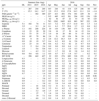
a.g.l.: above ground level; MBO: 2-methyl-3-buten-2-ol; SQT: sesquiterpene; MT: monoterpene; 4-AMCH: 4-acetyl-1-methylcyclohexene; MACR: methacrolein.
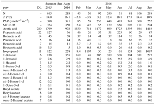
Table 2Mean concentrations of VOCs measured in summer (June–August) 2015 and 2016 (GC-MS2) and monthly mean concentrations (pptv) in February–September 2016 with mean temperature (T) and photosynthetically active radiation (PAR). N: number of measurements; DL: detection limit; “–” indicates a missing value.
2.3 Calculation of formation rates of measured reaction products of monoterpenes
To determine the diurnal variation in the measured reaction products of MTs, net formation rates (NFRs) were calculated. The production rate (PR), destruction rate (DR) and NFR of reactions products of MTs can be described by the equations below:
where k is the reaction rate coefficient of the MT or product with oxidant (hydroxyl radical, OH; or ozone, O3) and [MT], [product], [OH] or [O3] is the concentration of the corresponding MT, product or oxidant. In addition, the yields of the products from the corresponding reactions were used.
2.4 Reactivity calculations
The total reactivity of the VOCs (Rx) was calculated by combining their respective concentrations (individual VOC, VOCi) with the corresponding reaction rate coefficients (ki,x).
This determines in an approximate manner the relative role of compounds or compound classes in local OH, nitrate radical (NO3) and O3 chemistry. The experimentally determined reaction rate coefficients listed earlier by Praplan et al. (2018), Hakola et al. (2017) and by Ng et al. (2017) were used. When the experimental reaction rate coefficients were not available, the values estimated by the AopWin™ module of the EPI™ software suite (https://www.epa.gov/tsca-screening-tools/epi-suitetm-estimation-program-interface, last access: 27 September 2018, EPA, USA) as implemented online by ChemSpider (http://www.chemspider.com, last access: 27 September 2018; the Royal Society of Chemistry) were used. The estimation method used by AopWin™ is based upon the structure–activity relationship. All reaction rate coefficients are listed in the Supplement (Table S1). For the unknown SQTs average reaction rate coefficients ( cm3 s−1, cm3 s−1, cm3 s−1) of the known SQTs were used. Due to the lack of measured or estimated reaction rate coefficients, these average values were also used for longicyclene in the O3 and NO3 reactions and for β-farnesene in the NO3 reactions.
2.5 Calculation of total production rates of oxidation products
OxPRs were calculated for the reactions of the various VOCs with the OH, O3 and NO3 radicals by Eq. (5).
where k is the reaction rate coefficient of a VOC with an oxidant (OH, O3 or NO3) and [VOCi], [OH], [O3] or [NO3] is the concentration of the corresponding VOC or oxidant. Unknown SQTs were not taken into account in the calculations. Of the SQTs the reaction rate with NO3 radicals was found only for β-caryophyllene while the reactions of other SQTs were not considered in the calculations.
Since OH radical concentrations were not measured directly, proxies were calculated from the ultraviolet B (UVB) radiation intensity (Eq. 6), which is known to correlate strongly with OH radicals as first described by Rohrer and Berresheim (2006) and later evaluated by the observations at SMEAR II by Petäjä et al. (2009) and Hens et al. (2014).
Comparison with the measurements has shown that, even though the variation in concentrations was quite similar, this method results in concentrations 3 times higher than those of the measurements (Petäjä et al., 2009). Therefore, the OxPRs of the OH radical reactions were actually expected to be lower than those presented in this study.
The NO3 concentrations were calculated by assuming a steady state by its production from O3 and NO2 and removal by photolysis and oxidation reactions as described by Peräkylä et al. (2014). The only modification was that the data for individual MTs were used and β-caryophyllene (main SQT at the site) was also considered as an additional sink.
The aerosol surface area needed for the calculation of the NO3 concentration was derived from the aerosol number size distribution in the range 3–1000 nm at SMEAR II. It was obtained using two parallel differential mobility particle sizers (DMPS) (Aalto et al., 2001). Each DMPS system consisted of a Hauke-type differential mobility analyser (DMA) and condensation particle counter (CPC). Each DMA separated the sampled aerosol particles according to their electrical mobility, and the particles selected are transported to the corresponding CPC, which grew them by condensing butanol on their surface, and counted their number with optical methods. Particles with different electrical mobilities can be selected and counted by changing the strength of the electric field inside DMA. The first DMPS measured particles with sizes between 3 and 10 nm and the second between 10 and 1000 nm. In combining the spectra, the number size distribution of the entire size range was reached. One measurement cycle scanning all the sizes required about 10 min. Charging the aerosol population to an equilibrium charge distribution with a bipolar charger enabled the measurements of both neutral and charged particles.
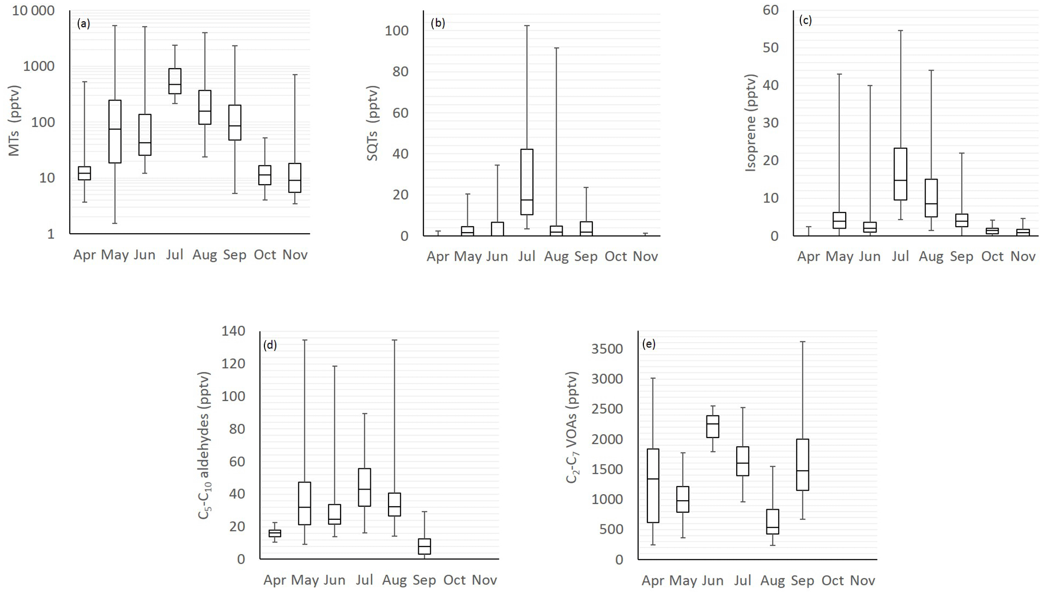
Figure 1Monthly mean box and whisker plots of (a) monoterpenes (MTs), (b) sesquiterpenes (SQTs), (c) isoprene, (d) C5–C10 aldehydes and (e) C2–C6 volatile organic acid (VOA) concentrations. The boxes represent first and third quartiles and the horizontal lines in the boxes the median values. The whiskers show the highest and lowest observations. Note that the y axes for the MTs are in a logarithmic scale.
The number of particles in a unit volume in a certain size range can be determined as
where n(log Dp) is the number density distribution representing the number of particles between diameter Dp and Dp+dDp per unit volume. If all the particles are assumed to be spherical, the surface area distribution becomes
Then the surface area of the particles in the range is obtained similarly as
2.6 Complementary measurements
The meteorological data, O3, NO and NOx concentrations were obtained from the SmartSMEAR AVAA portal (Junninen et al., 2009, https://avaa.tdata.fi/web/smart, last access: 27 September 2018). All the data used in this study are those collected at a height of 4.2 m from the mast inside the forest, except for the temperature, which was collected at 125 m for comparison.
The mixing layer height (MLH) was estimated from measurements with a Halo Photonics Stream Line scanning Doppler lidar, which is a 1.5 µm pulsed Doppler lidar with a heterodyne detector (Pearson et al., 2009). The range resolution of the lidar is 30 m and the minimum range of the instrument is 90 m. Operating specifications of the lidar are given in Supplement Table S2. The wind profile at Hyytiälä was obtained from a 30∘ elevation angle conical scan, i.e. from a vertical azimuth display (VAD) scan. This VAD scan was configured with 23 azimuthal directions and integration time of 12 s per beam. A vertical stare of 12 beams and integration time of 40 s per beam was configured to follow the VAD scan. The VAD scan and 12-beam vertical stare were scheduled every 30 min at Hyytiälä; other scan types operated during the 30 min measurement cycle were not utilised in this study. The lidar data were corrected for a background noise artefact according to Manninen et al. (2016). After this correction a signal-to-noise-ratio threshold of 0.001 was applied to the data.
The turbulent kinetic energy (TKE) dissipation rate was calculated from the Doppler lidar measurements according to the method by O'Connor et al. (2010). A VAD-based proxy for turbulent mixing () was calculated from the 30∘ elevation VAD scan according to the method by Vakkari et al. (2015). The MLH was determined from the TKE dissipation rate and the VAD scan in a manner similar to that of Vakkari et al. (2015). Briefly, a constant threshold of 10−4 m2 s−3 was first applied to the TKE dissipation rate profile; i.e. the MLH was taken as the last range gate where the TKE dissipation rate was higher than 10−4 m2 s−3. If the TKE dissipation rate was below the threshold value at the first usable gate at 105 m above ground level (a.g.l.), i.e. MLH <105 m, the profile was used to identify the MLH. For a constant threshold of 0.05 m2 s−2 was applied to determine the MLH (Vakkari et al., 2015). With this approach, the MLH could be identified from 60 to >2000 m a.g.l.; rainy periods were excluded from the analysis. Values below 60 m were marked as 0 m.
3.1 Seasonal and diurnal variations in concentrations
The concentrations of most compounds measured with three different GC-MS instruments in 2011, 2015 and 2016 were similar (Tables 1 and 2). Of the compounds measured the VOAs showed the highest concentrations during all months (Fig. 1, Tables 1 and 2). The 1-butanol and isopropanol concentrations were also high, most likely because they were used in some instruments for aerosol measurements at the site. Even though the concentrations of the terpenoids were not as high as those of the VOAs due to their high reactivity, they were expected to show the greatest impacts on local chemistry. For most of the compounds studied, daily and monthly mean concentrations were highest during the warm summer months. For aromatic hydrocarbons, which are mainly emitted from anthropogenic sources, the concentrations were higher in winter.
The relative diurnal variation in most compounds was highest in June when the MLHs were highest (Figs. 2 and 3). The concentrations of the various compounds and compound classes are described in further detail in the following sections.
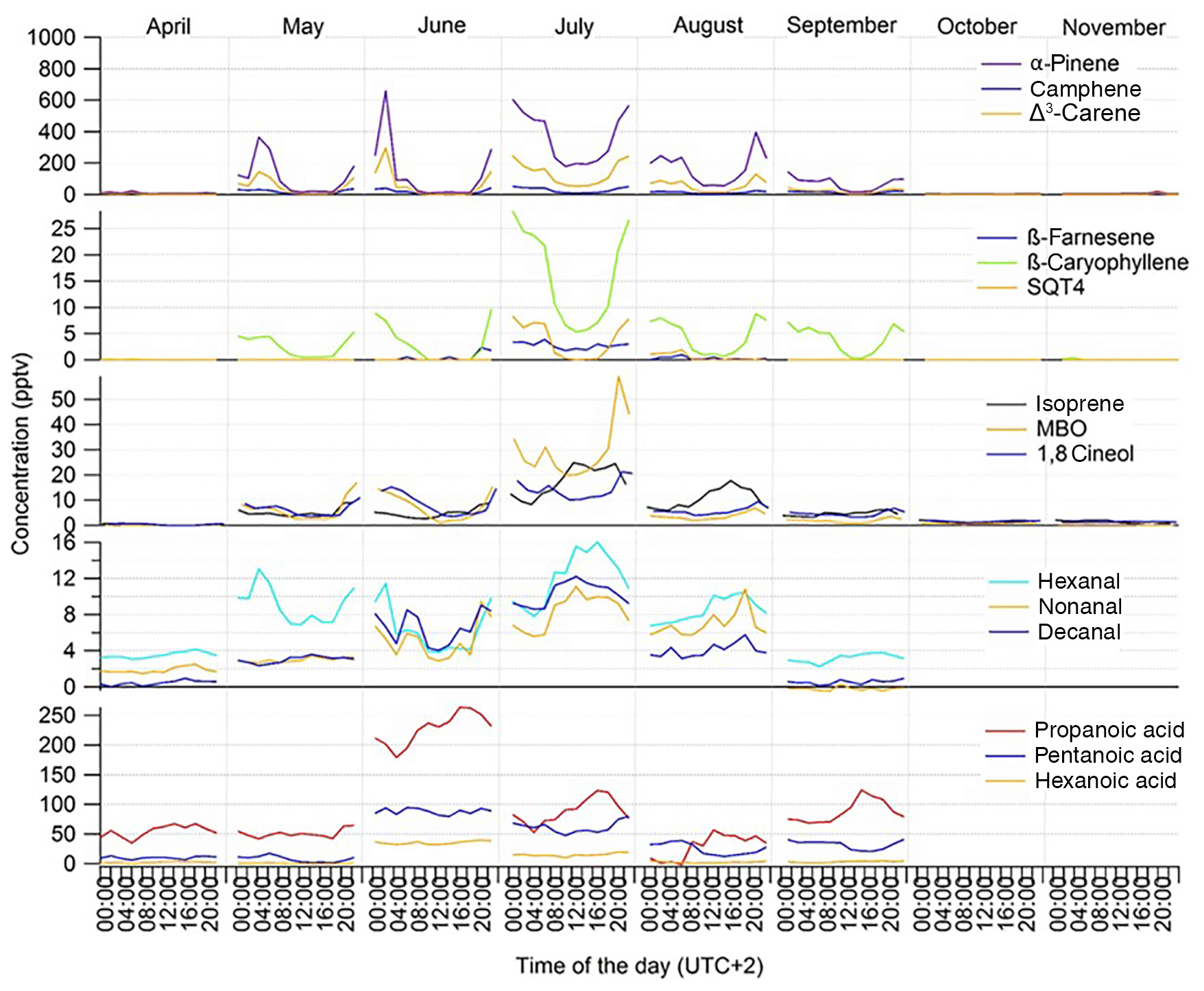
Figure 2Monthly mean diurnal variation of concentrations of different VOCs at the SMEAR II station in 2016.

Figure 3Monthly mean diurnal variation in meteorological parameters and concentrations of main oxidants (OH radical, O3 and NO3 radical) in 2016 during the GC-MS3 measurement periods. PAR: photosynthetically active radiation; WS: wind speed at the height of 8.4 m; MLH: mixing layer height; Tdiff: temperature difference between heights of 125 and 4.2 m; RH: relative humidity; precipint: intensity of precipitation. WS data for September–November and NO3 radical and RH data for October are missing.
3.1.1 Concentrations of monoterpenes
The MTs showed the highest concentrations of the terpenoids, with the mean MT sum being 400, 440 and 430 pptv in summers (July–August) 2011, 2015 and 2016, respectively (Table 1). All the MTs except p-cymene showed clear maxima in summer. p-Cymene is also known to have anthropogenic sources (Hakola et al., 2012). The variations in the MT sum measured with the GC-MS2 and GC-MS3 were similar (Fig. S1 in the Supplement), but their direct comparison was not possible, due to the different sampling times.
Long-term MT concentration measurements were previously conducted at this boreal forest site with PTR-MSs (Lappalainen et al., 2009; Kontkanen et al., 2016). Those PTR-MS measurements were conducted close to the forest canopy at heights of 14 m (2006–2009) or 16.8 m (2010–2013). The median July MT concentration measured between 2006 and 2013 was 382 pptv. In previous studies in March 2003, 2005 and 2006, the MT concentrations measured in short campaigns with PTR-MSs have been higher than in our measurements in April 2016 (Table S3). Yassaa et al. (2012) measured concentrations lower than ours in a campaign in July–August 2010. Large spatial differences in concentrations especially for terpenoids were expected depending on the sampling point at the site (Liebmann et al., 2018). In our study the sampling site was at the edge of the forest whereas in previous studies by Lappalainen et al. (2009) and Kontkanen et al. (2016) it was in the upper canopy level and in Yassaa et al. (2012) above at the canopy at a height of 24 m, where it is expected, due to transport and chemistry, that concentrations are lower compared to our measurements.
In our measurements, the MT concentrations showed high peaks in May 2016 (12 May at 03:04 and 14 May at 04:10–06:10), 1 June at 01:10 and 9 September at 23:35, which clearly deviated from the other data. Based on the wind directions, these peaks may have been due to high concentrations coming from the site of operations of a sawmill, a wood mill and a pellet factory in Koreakoski, 5 km southeast of Hyytiälä. The influence of this factory on the MT concentrations has also been observed previously (Eerdekens et al., 2009; Liao et al., 2011; Williams et al., 2011; Hakola et al., 2012). These samples were not used in further analysis.
α-Pinene showed the highest concentration of the measured MTs (50 % of the MT sum) followed by Δ3-carene, β-pinene and limonene (Table 1). The MT distribution was very similar for nighttime (photosynthetically active radiation, PAR, <50 µmol s−1 m−2) and daytime (PAR >50 µmol s−1 m−2); only 1,8-cineol and linalool showed slightly higher fractions during the day. Similar MT distributions have also observed at the site (Hakola et al., 2012; Yassaa et al., 2012) and resemble one of the emissions of local trees (Bäck et al., 2012; Hakola et al., 2006, 2017).
The diurnal variability in the MT concentrations at the site was driven by vertical mixing; low values were measured during the day when mixing was highest and the highest values during nights with the lowest mixing (Figs. 2 and 3). This has been observed also in earlier studies of MTs at this boreal forest site (Hakola et al., 2012; Kontkanen et al., 2016). Similar diurnal variation was found by Bouvier-Brown et al. (2009) in a ponderosa pine forest in the Sierra Nevada Mountains of California. However, this observation of MTs is in contrast to the diurnal variation in MT concentrations measured in the Amazon tropical rainforest by Yáñez-Serrano et al. (2017). Light-dependent emissions found in the Amazon rainforest (Jardine et al., 2015) could explain this. In boreal forests emissions are strongly temperature dependent and may also continue during nights with only lower rates if temperature is sufficiently high (e.g. Hakola et al., 2006).
The diurnal variation in concentrations was highest in June, concomitant with the highest variation of the MLH (Figs. 2 and 3). The MLHs during the day (at 12:00–16:00) in June and July were 1605 and 819 m, respectively, while during the night (at 00:00–04:00) in June and July they were 87 and <60 m, respectively. The monthly mean MLH, which roughly describes the mean dilution volume of the emissions, was also twice as high during our measurements in June than in July (Table 1). Since the lidar used for measurements of the MLHs was unable to detect MLHs <60 m, we also used temperature difference between heights 125 and 4.2 m to roughly describe the vertical mixing. The correlation of monthly mean diurnal variation in MT sum concentrations with temperature differences at the site was high ( in July). Individually measured values also showed relatively favourable correlation with temperature difference ( in July, Fig. S2b). 1,8-Cineol and linalool did not follow this general diurnal pattern of MTs indicating different sources. 1,8-Cineol is the only MT known to also show clearly light-dependent emissions from Scots pines growing at the site (Hakola et al., 2006).
3.1.2 Concentrations of sesquiterpenes
Few data are available on atmospheric SQT concentrations and emission data are also much sparser than for MTs. In our measurements SQTs showed seasonal variation similar to that of the MTs, but their concentrations were much lower (Table 1). SQTs are very reactive and therefore their contribution to the local chemistry can still be significant. The highest 30 min mean for the SQT sum (103 pptv) was detected on 25 July at 03:15, coinciding with high temperature and a shallow mixing layer. The concentrations of SQTs did not increase during the sawmill episode, in contrast to that observed for MTs. They were more reactive and, if emitted, were probably depleted during transport from the sawmill to the site.
β-caryophyllene showed the highest concentrations among the SQTs measured followed by longicyclene, β-farnesene and four unidentified SQTs detected only in July and August (Table 1). Nighttime (PAR <50 µmol s−1 m−2) and daytime (PAR >50 µmol s−1 m−2) distributions of SQT concentrations were very similar; only β-farnesene showed a slightly higher fraction during the day. β-caryophyllene is emitted by local pines and spruces (Hakola et al., 2006, 2017) as well as from the forest floor (Hellén et al., 2006; Mäki et al., 2017; Bourtsoukidis et al., 2018). Aaltonen et al. (2011) and Mäki et al. (2017) also detected longicyclene in forest floor emissions. Laboratory studies have shown stress-related emissions of β-farnesene (Petterson, 2007; Blande et al., 2009), and β-farnesene was also detected in local spruce emissions by Hakola et al. (2017).
The diurnal variation in most SQTs was similar to the variation in MTs, and the concentrations were largely driven by vertical mixing (Figs. 2 and 3). As for the MTs, correlation of the monthly mean diurnal variation in the SQT concentrations with temperature difference between the heights of 125 and 4.2 m was high ( in July) while individual measured values also showed relatively favourable correlation with the temperature difference ( in July, Fig. S2b). In addition to mixing, a higher chemical sink compared to MTs may affect local SQT concentrations during the day (Zhou et al. 2017). This was supported here by the higher relative diurnal variation in SQTs compared to MTs. The only exception was β-farnesene, which showed almost as high concentrations during the day as at night, indicating different sources than for different SQTs and MTs. A contrasting diurnal variation was found by Bouvier-Brown et al. (2009) in a ponderosa pine forest in California, suggesting that the sources of β-farnesene are mainly light dependent.
3.1.3 Isoprene and 2-methyl-3-buten-2-ol concentrations
The isoprene and 2-methyl-3-buten-2-ol (MBO) concentrations were low (Table 1). Low concentrations of isoprene have also been observed in previous studies (Table S3). In our study, the monthly means in 2016 were 0.3–18 pptv for isoprene and 0.1–30 pptv for MBO. Low levels were expected since the main local trees (Scots pine and Norway spruce) are MT emitters and show only minor emissions of isoprene and MBO (Tarvainen et al., 2005; Hakola et al., 2006, 2017). The highest daily means were measured in July and August together with MTs and SQTs. The emissions of isoprene are light dependent (Ghirardo et al., 2010) while MBO emissions from local trees are mainly temperature dependent (Hakola et al., 2006).
The diurnal variation in MBO coincided with the variation in MTs, with high values during the night and low values during the day. This was expected, due to the temperature-dependent emission of MBO. For isoprene, clear changes in diurnal variation were observed between early summer (April–June) and late summer (July–September) (Fig. 2). In May and June, when emissions are still low due to the early growing season, lower daytime values were detected, but in July and August the daytime concentrations were clearly higher due to high light-dependent emissions. Previously, the gradually increasing isoprene emissions have been associated with the foliage growth period and start when the effective temperature sum (ETS) reaches a threshold value. For example, in tea-leaved willow (Salix phylicifolia L.), lower emissions of isoprene were found when the ETS <400∘ days (Hakola et al., 1998). During our measurements in 2016, the ETS reached a value 400 on 23 June.
3.1.4 Concentrations of reaction products of terpenes
Methacrolein (MACR) is a reaction product of isoprene, but the monthly average MACR concentrations did not follow the concentrations of its precursor isoprene (Table 1). MACR may also have anthropogenic sources (Biesenthal and Shepson, 1997) and in spring and autumn, when lifetimes are longer and biogenic emissions lower than in summer, anthropogenic influence was expected to be higher. In their studies Biesenthal and Shepson (1997) found that the MACR concentrations near Vancouver were not explained by the photochemical source, while in Toronto MACR correlated with carbon monoxide (CO), suggesting they originate in traffic emissions. In our study, the monthly mean concentrations of MACR (4.8 and 3.3 ppt, respectively) were ca. 30 % of the isoprene concentration in July and August when the isoprene concentrations and biogenic emissions are highest. This is similar to the yields of 25 % and 24 % measured in chamber experiments by Paulson et al. (1992) and Atkinson (1994), respectively.
Nopinone is a reaction product of β-pinene and its monthly mean concentration followed the variation in MTs (Table 1). During the summer months its concentration was 7–13 % of the concentration of its precursor β-pinene. In reaction chamber studies, the yields of nopinone in O3 reactions of β-pinene have been 19–23 % (Grosjean et al., 1993; Hakola et al., 1994; Winterhalter et al., 2000) and in OH radical reactions 25–37 % (Calvert et al., 2011; Kaminski et al., 2017).
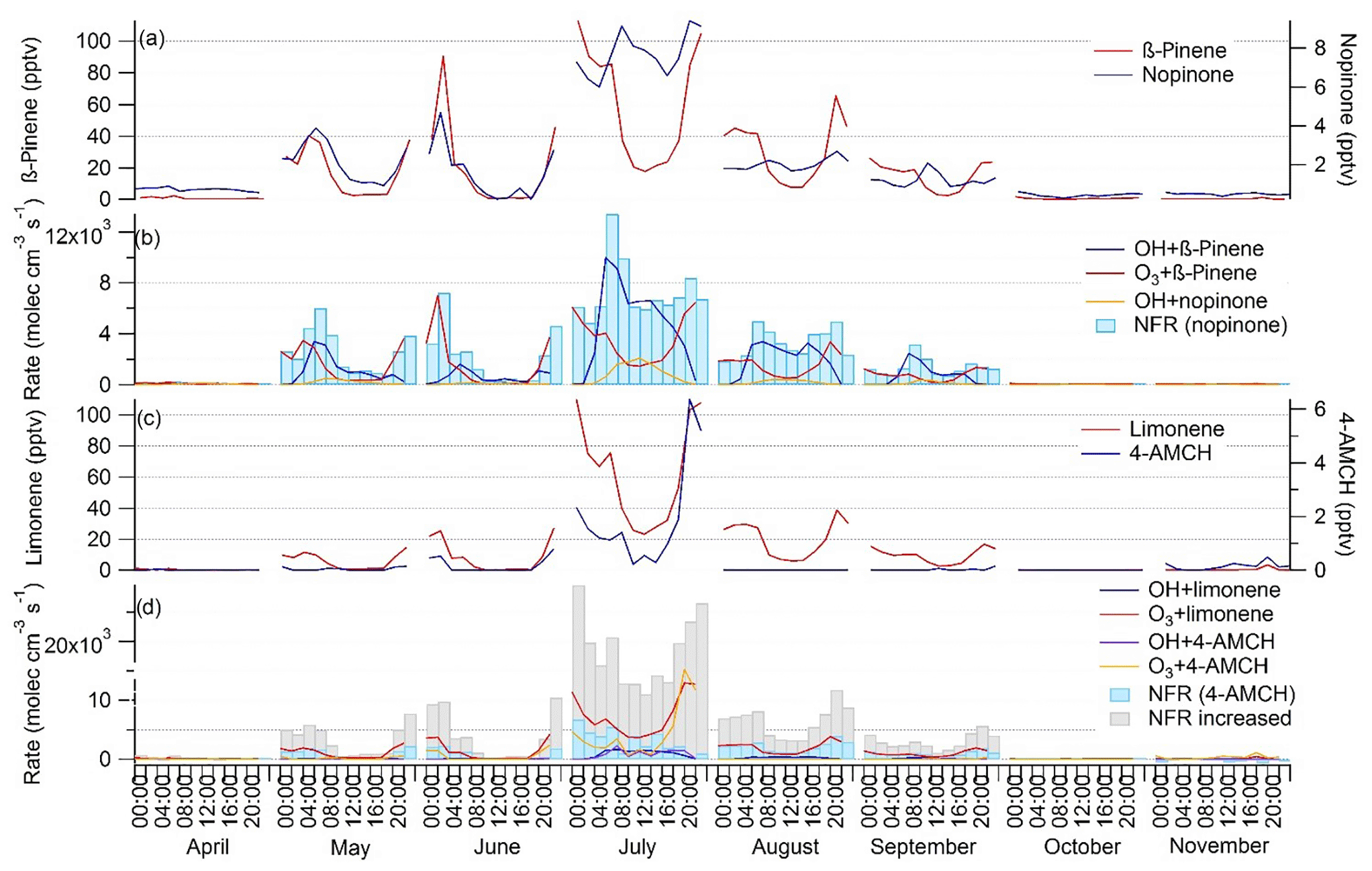
Figure 4Monthly mean diurnal variation in (a) β-pinene and nopinone concentrations; (b) production rates of nopinone from OH (OH +β-pinene) and O3 (O3+β-pinene) reactions, destruction rate of nopinone by OH reaction (OH + nopinone) and net formation rates (NFR) of nopinone; (c) limonene and 4-acetyl-1-methylcyclohexene (4-AMCH) concentrations; and (d) production rates of 4-AMCH from OH (OH + limonene) and O3 (O3 + limonene) reactions, destruction rates of 4-AMCH by OH (OH + nopinone) and O3 (O3 + 4-AMCH) reactions, as well as NFR and NFR with increased yields (NFR increased) of 4-AMCH.
The mean diurnal variation in nopinone followed the variations in its precursor (β-pinene) in April–June, but in July–September high values were also observed during the day (Fig. 4). Nopinone is known to be produced both in OH radical and O3 reactions of β-pinene (Hakola et al., 1994), but it is destroyed only in the OH radical reactions. Since the yields from the NO3 radical reactions are not available in the literature, they cannot be considered. The NO3 reactions would increase production especially at night. Deposition may also have an effect (Zhou et al., 2017), but it was not taken into account here. The PR, DR and NFR of nopinone were calculated using the Eqs. (1)–(3). The nopinone yields used for OH radical and O3 reactions obtained from Hakola et al. (1994) were 0.27 and 0.23, respectively. Change in the nopinone diurnal variation is explained by the balance between its sources and sinks. The concentrations closely followed the NFR variation (Fig. 4). Nopinone is a rather stable molecule and has 5 times lower OH radical reactivity than β-pinene and, in contrast to β-pinene, it does not react with O3. The results indicate that in May and June, when there was already high light intensity and high OH radical concentrations, but the emissions of β-pinene were still low due to lower temperatures and an early growing season, the nopinone produced may have reacted away during the day, while higher values were measured during the night, when there are no OH radicals, but nopinone is still produced from O3 reactions of β-pinene. In July and August higher emissions and more rapid reactions of β-pinene with OH radicals resulted in higher daytime concentrations of nopinone. In September the emissions were already lower, but the OH radical concentrations and MLHs were also lower, while higher nopinone concentrations were still detected during the day.
The reaction product of limonene, 4-acetyl-1-methylcyclohexene (4-AMCH), showed very low concentrations and was detected only in June and July (Table 1). The NFR for 4-AMCH was calculated by the same methods as for nopinone using Eqs. (1)–(3). The reaction rates of 4-AMCH with the OH radical and O3 were only 25 % and 20 % lower than for its precursor. The 4-AMCH yields used here for the OH radical and O3 reactions obtained from the Hakola et al. (1994) were 0.20 and 0.04, respectively. In a study by Grosjean et al. (1993) the yield from the O3 reaction was 0.02. The concentrations measured in the present study did not follow the diurnal variation in the NFR, especially in July, when the highest concentrations were measured (Fig. 4). However, PR showed a diurnal pattern similar to that of the concentrations. Studies on limonene reactions by Grosjean et al. (1993) and Hakola et al. (1994) did not take into account that 4-AMCH reacts almost as rapidly with the oxidants as limonene and that the real yields could have been higher. When we increased the yields in our calculations, better agreement was achieved. In Fig. 4d the yields for the OH radical and O3 reactions were increased by factors of 2 and 3, respectively. In August, the sensitivity of the instrument was less than 50 % of the sensitivity in June and July, due to faulty tuning of the MS, and 4-AMCH was not detected even though calculations indicated higher concentrations than in June.
3.1.5 Concentrations of volatile organic acids
The VOAs showed higher concentrations than terpenoids (Tables 1 and 2). Their atmospheric lifetimes (Calvert et al., 2011; Hellén et al., 2017) are much longer and therefore they can accumulate in the atmosphere and be transported for longer distances. They were expected to have both biogenic and anthropogenic sources and they are also produced in the atmosphere by the reactions of other VOCs (Ciccioli and Mannozzi, 2007). In the present study, the highest concentrations of VOAs in 2016 were already measured in June (Table 2). This was at least partly due to the different measurement periods for the GC-MS2 and GC-MS3 in June and July. The days when the VOAs were measured with the GC-MS2 were in late June when the temperature (18 ∘C) and PAR were higher than VOC measurements with GC-MS3 in June (temperature 12 ∘C). The MT sum measured together with the VOAs also showed the highest monthly mean in June.
The daily means of C3–C7 VOAs were more highly correlated with the MT sum (R=0.6–0.85) than with anthropogenic compounds such as toluene (R=0.0–0.31), indicating the biogenic origin of these compounds, either directly or through secondary production in the atmosphere. Only acetic acid showed some correlation with aromatic hydrocarbons (R=0.2–0.48). Since the lifetime of acetic acid is longest (1–2 weeks; Calvert et al., 2011), it was expected to be more influenced by the long-range-transported anthropogenic emissions.
The daily means of hexanoic acid were very highly correlated not only with 1-hexanol (R=0.97), but also with other C6 compounds often referred to as green leaf volatiles (GLVs), e.g. hexanal (R=0.82) and cis-3-hexenol (R=0.83). This indicates that hexanoic acid could also be a GLV or that it is produced from GLVs in the atmosphere. Correlation of the daily means of hexanoic acid with pentanoic and propanoic acids was also high (R=0.89 and 0.80, respectively) and with the MT sum relatively high (R=0.77).
For smaller acids (acetic, propanoic and butanoic) daytime maxima were observed, especially in July and August, but for pentanoic and hexanoic acids higher concentrations were observed at night (Fig. 2). The mean diurnal variation in VOAs was not as strong as for the MTs and SQTs. Both direct biogenic emissions and production in the atmosphere were expected to be higher during the day, but since the mixing layer was also higher the VOAs were more diluted. However, due to the longer lifetimes of these acids, the mixing effect during the day was not as strong as for fast-reacting terpenes since the background air may also have contained comparable amounts of these acids. These acids may be transported from distant sources or produced in the upper parts of the mixing layer from the reactions of other VOCs. The losses due to OH reactions during the day and dry/wet deposition during nights were also expected to affect the concentrations (Calvert et al., 2011). In canopy-scale flux measurements by proton-transfer-reaction time-of-flight (PTR-TOF) devices, downward fluxes of acetic acid have been detected, especially at night (Schallhart et al., 2018).
3.1.6 Concentrations of C5–C10 aldehydes
C5–C10 aldehydes can be directly emitted or they can be produced in the atmosphere through oxidation of other compounds. Generally, the emissions are much lower than those of smaller aldehydes. Low emissions have been measured, e.g. from grasslands, but emissions of trans-2-hexenal, 2-hexenyl acetate and 2-hexenol from damaged and stressed plants can be significant (Fall, 1999; Hakola et al., 2001). Possanzini et al. (2000) found that larger aldehydes (heptanal, octanal) were emitted from citrus plants when exposed to O3. There is also some evidence that nonanal can be produced when O3 attacks the fatty acids on leaf or needle surfaces (Bowman et al., 2003). Hakola et al. (2017) also measured C4–C10 aldehyde emissions from Norway spruce and found that their magnitudes were similar to that of MT emissions during late summer.
The concentrations of C5–C10 aldehydes were low; their monthly means remained <10 pptv (Table 1). In the measurements of Hellén et al. (2004) at the same site in March and April 2003, the concentrations were slightly higher (12–16 pptv) but similar. The diurnal variations in C5–C10 aldehydes followed the variation in isoprene, with low daytime values in June and high values in July and August (Fig. 2).
The daily means of hexanal were highly correlated with MTs and SQTs (R=0.90) in summer (June–August). The daily means of nonanal and decanal showed the highest correlation with β-farnesene in summer. Since β-farnesene emissions are related to stress, this could also have indicated stress-related sources for the emissions.
In July, 24 h samples for analysis of carbonyls with a liquid chromatograph (LC, Praplan et al., 2018) were collected concomitant with the GC-MS3 measurements, similar to Praplan et al. (2017). The concentrations of <C5 carbonyls were also obtained from those samples. The July means for formaldehyde, acetaldehyde, acetone and butanal were 430, 270, 1820 and 50 pptv, respectively. The concentrations of these smaller carbonyls were much higher than for the C5–C10 aldehydes. This was expected due to their longer lifetimes and larger emissions (Hellén et al., 2004).
The formation of aldehydes in GC and PTR-MS instruments from organic peroxides has been discussed (Rivera-Rios et al., 2014). However, we measured MACR and hexanal with both LC and the GC-MS3 in July 2016 and the results were comparable (MACR 4.7 and 4.8 pptv and hexanal 8.4 and 12 pptv, respectively). For pentanal even higher concentrations were obtained by LC (July mean 45 ppt). In 2015 when the GC-MS1 was used, the aldehyde concentrations were clearly higher than in 2016 (Table 1) and production from organic peroxides in the GC-MS1 may explain the difference. This indicates that the hypothesis by Rivera-Rios et al. (2014) may hold for some GC instruments, but it is still unclear under which circumstances.
3.1.7 Concentrations of alcohols and acetates
C4–C8 alcohols and acetates (including GLVs) generally show very low concentrations; the monthly means were mostly below the detection limits (Table 2). The only exceptions were 1-butanol and isopropanol, both of which were used in instrumentation at the site and therefore showed higher concentrations from leaks and exhaust lines. As for the other BVOCs the highest concentrations of most alcohols and acetates were measured in summer. Most of the alcohols and acetates measured were GLVs, which are emitted due to herbivory or pathogen infection by almost every green plant (Scala et al., 2013) or due to physical damage of plants (Hakola et al., 2001).
3.2 Correlation of concentrations with temperature
The monthly and daily means of most of the BVOCs examined correlated exponentially with temperature. This temperature dependence is described in further detail for different compound groups as well as for individual BVOCs in the following sections.
3.2.1 Correlation of monoterpene concentrations with temperature
The monthly mean MT concentrations showed very strong exponential correlation with temperature (R2=0.92, Fig. 5a). The site is dominated by Scots pines, which have temperature- and light-dependent emissions of MTs (Tarvainen et al., 2005). The PAR was highly correlated with monthly mean MT concentrations (), but correlation was clearly lower than with temperature.
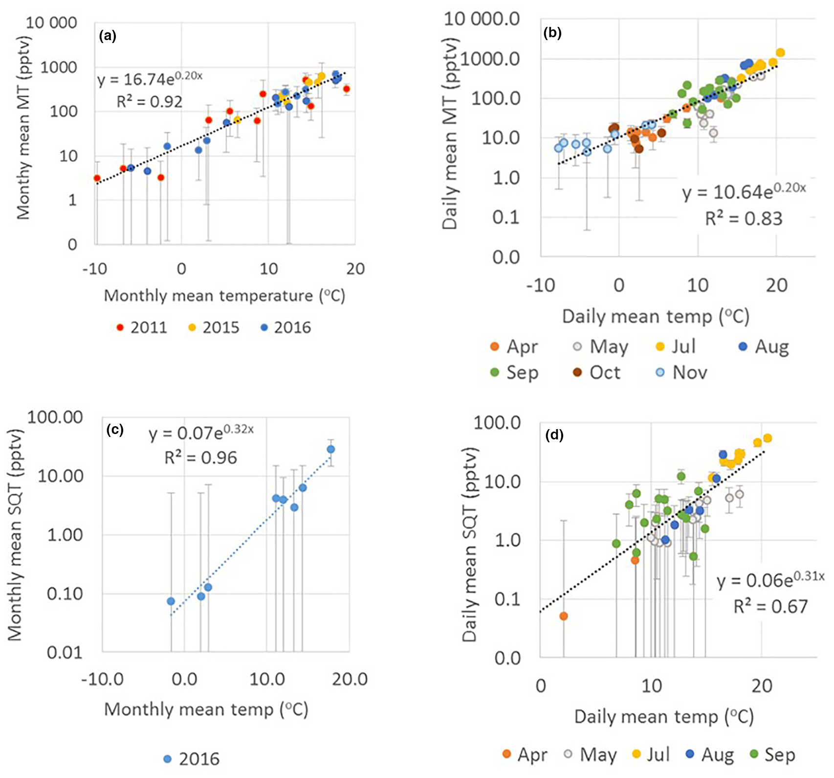
Figure 5Exponential correlation of temperature with (a) monthly mean MT concentrations in 2011, 2015 and 2016; (b) daily mean MT concentrations in 2016; (c) monthly and (d) daily mean SQT concentrations in April–November 2016 measured at SMEAR II. Error bars show the uncertainty of the mean concentrations calculated from the uncertainty of the measurements. Note that the y axes are in a logarithmic scale.
The daily mean MTs also correlated well with temperature ( and , Table 3 and Fig. 5b). The high correlation with temperature observed indicates that temperature has a major effect on the seasonality of the concentrations and emissions and processes controlling them. In a previous study by Lappalainen et al. (2009) lower correlation (R2=0.50) with temperature was found for the PTR-MS data. However, they used only daytime medians. In our study 24 h averages starting at 08:00 (UTC+2) and ending the next day at 08:00 (UTC+2) were used.
Table 3Correlation of VOC concentrations with temperature at SMEAR II in 2016, intercept (α) of temperature dependence curve, temperature sensitivity (β), and temperature correlations (R2) of monthly (April–November) and daily (June–August) mean concentrations and mixing layer height (MLH)-scaled concentration of individual measurement points (CMLH). The fitted curves were exponent functions y=αeβx, where y is the concentration or MLH-scaled concentration, x is the temperature and β is the temperature sensitivity.
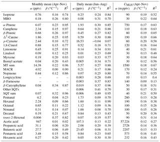
MBO: 2-methyl-3-buten-2-ol; MACR: methacrolein; MT: monoterpene; SQT: sesquiterpene.
Temperature dependence of MT emissions is often described by the Guenther algorithm (Guenther et al., 1993):
where ES is the standardised emission potential (µg g−1 dry weight (dw) h−1), T the leaf temperature (∘C), TS the standard temperature of 30 ∘C and β the temperature sensitivity (∘C−1) of the emissions. Often the value 0.09 ∘C−1 is used for β to describe MT emissions. In our monthly and daily mean concentration data, the temperature sensitivity was clearly higher (β=0.20 ∘C−1, Fig. 5 and Table 3). The temperature also affects the vertical mixing of air, and a lower mixing after warm sunny days probably increased the temperature sensitivity of the concentrations. Even though the value 0.09 ∘C−1 is often used for β to model emissions, it is known to vary (Hakola et al., 2006). Here the temperature sensitivity of the daily mean MT concentration for the summer months (β=0.27 ∘C−1, June–August) was also higher than for the entire growing season (β=0.20 ∘C−1, April–November).
To determine the temperature sensitivity of the individual MTs, data from the GC-MS3 were used. Exponential correlations of the monthly means with temperature showed that R2>0.91 (Table 3 and Fig. S3) for all monoterpenoids except 1,8-cineol (R2=0.77), p-cymene (R2=0.72), bornyl acetate (R2=0.71) and linalool (R2=0.25). Tarvainen et al. (2005) found that, in Scots pine emissions, 1,8-cineol was the only MT that was both light and temperature dependent while the others were only temperature dependent. p-Cymene has been detected for example in Norway spruce emissions (Hakola et al., 2017), but it also has anthropogenic sources (Hakola et al., 2012). Linalool is emitted by trees as a result of biotic stress (Petterson, 2007; Blande et al., 2009). Bornyl acetate, linalool and 1,8-cineol showed very low concentrations, which also resulted in higher uncertainty. For the MTs with high (R2>0.91) temperature correlation, the β values of the monthly means varied between 0.15 and 0.26 ∘C−1, with the values being lowest for camphene and highest for β-pinene.
3.2.2 Correlation of sesquiterpene concentrations with temperature
As for the MTs, the monthly and daily means of the SQTs also showed very strong exponential correlation with temperature (Table 3, Fig. S4). The temperature sensitivity of the SQTs was even higher than for MTs. The SQT emissions from Norway spruce (Hakola et al., 2017) and Scots pine (Tarvainen et al., 2005) were closely correlated with temperature, but the SQT emissions may also have been influenced by light (Duhl et al., 2008). The daily mean β-caryophyllene concentrations showed very high exponential correlation with temperature () supporting only temperature-dependent emissions. The monthly means of the SQT sum (consisting mainly of β-caryophyllene) also showed very high exponential correlation with temperature (R2=0.97), indicating that seasonality is also driven by the temperature. For the other SQTs, the correlations were lower than for β-caryophyllene. Low concentrations with higher measurement uncertainty and light- and stress-related emissions may have significantly affected the correlations. β-Farnesene is emitted due to biotic stress (Kännaste et al., 2009) and increases simultaneously with linalool in the emissions of Norway spruce and Scots pines (Hakola et al., 2006, 2017). However, the linalool and β-farnesene concentrations did not correlate in our data. Bouvier-Brown et al. (2009) suggested that at least in a ponderosa pine forest β-farnesene emissions may be both temperature and light dependent.
3.2.3 Correlation of isoprene and 2-methyl-3-buten-2-ol concentrations with temperature
Isoprene emissions are both light and temperature dependent (Guenther et al., 1993; Ghirardo et al., 2010). Here correlation of the isoprene daily mean concentrations with light and the temperature activity factor (Guenther et al., 1993) was slightly lower (R2=0.74) than for the temperature only (R2=0.84, Fig. S5). However, the difference in R2 is small and, since the concentrations were low and close to the detection limits, no clear conclusions can be drawn from this. The MBO was somewhat better correlated with light and the temperature activity factor (R2=0.76) than with temperature only (R2=0.70). This is in contrast to the Scots pine emissions, in which the MBO was only temperature dependent (Tarvainen et al., 2005).
Even though the diurnal variation in most MT, SQT and MBO concentrations did not follow the ambient temperature, isoprene showed the highest concentrations during the day, while the 30 min mean concentrations were exponentially correlated with the ambient temperature (Fig. S6, R2=0.64). Due to the close link between isoprene production and light, isoprene is produced and emitted from trees only during the light hours and is therefore detected in the atmosphere only during the day while the MBO, MTs and SQTs are also emitted from storage pools inside the needles or leaves during the night, and due to lower vertical mixing the ambient air concentrations are higher at night (Ghirardo et al., 2010).
3.2.4 Correlation of terpenoid reaction product concentrations with temperature
The nopinone concentrations showed very clear exponential correlation with temperature () due to the temperature dependence of its precursor (β-pinene) and more rapid production on warm and sunny summer days. The temperature sensitivity of the nopinone daily means (β=0.25 ∘C−1) is similar to the sensitivity of its precursor β-pinene (β=0.27 ∘C−1).
MACR, which is a reaction product of isoprene, was as highly correlated (R2=0.86) with temperature in summer as its precursor isoprene (R2=0.84) but the temperature sensitivity was slightly lower (βisoprene=0.24 ∘C−1 and βMACR=0.17 ∘C−1). Similar to its precursor, the 30 min mean concentrations of MACR also showed low exponential correlation with temperature (R2=0.32, Fig. S6), but the monthly means of MACR did not correlate with temperature (R2<0.01, Table 3).
3.2.5 Correlation of oxygenated volatile organic compound concentrations with temperature
Since the concentrations of most C5–C10 aldehydes were very close to the detection limits, the results are more scattered but still clearly show strong correlation with the temperature. The highest correlation of the daily means in summer (June–August) was found for hexanal (R2=0.90) and the lowest for octanal (R2=0.36) and decanal (R2=0.43, Table 3 and Fig. S7). The temperature sensitivities of the aldehydes (β=0.08–0.13 ∘C−1) were clearly lower than for terpenoids (β=0.18–0.67 ∘C−1). Aldehydes have direct biogenic emissions (Seco et al., 2007; Hakola et al., 2017), but they are also produced in the atmosphere by the oxidation of other VOCs. The correlation of the daily mean concentrations of trans-2-hexenal with the light and the temperature activity factor (Guenther et al., 1993) was higher (R2=0.71) than only with temperature (R2=0.57), indicating a light-dependent source.
As for the isoprene and its reaction product MACR, the diurnal variations in pentanal and hexanal concentrations were also correlated with temperature and temperature sensitivities for the 30 min mean concentrations (βpentana=0.07 ∘C−1 and βhexanal =0.08 ∘C−1, Fig. S6b), similar to that of MACR (βMCAR=0.06 ∘C−1). This indicates that photochemical reactions could be an important source for these compounds as well.
A weak correlation with temperature was also found for the VOAs, but it was lower than for most other VOCs studied (Table 3). Due to the long lifetime of VOAs, the background concentrations and anthropogenic sources were expected to have more of an effect on the concentrations, and therefore their effect of local temperature-dependent emissions and production in the atmosphere remains unclear. Correlation of the daily means was highest for pentanoic acid (R2=0.65, Table 3, Fig. S7). The temperature sensitivity of the butanoic acid daily means (β=0.06 ∘C−1) was lower than for the other VOAs. The butanol concentrations at the site were strongly affected by the emissions from the particle counters used and were expected to produce butanoic acid.
3.2.6 Seasonality of temperature correlations
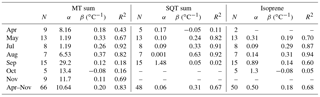
The variation in the daily mean concentrations is best explained by the temperature in summer (Table 4). The temperature sensitivity of the MT, SQT and isoprene concentrations was highest during the summer months and lower in autumn and spring. In summer, the emissions from trees were expected to play a major role, but in spring and autumn the relative impact of other emissions (e.g. sawmill emissions) increased.
Table 4Characterisation of the temperature dependence of the isoprenoid concentrations with intercept (α), temperature sensitivity (β) and correlation (R2) of the daily mean concentrations of MT sum and SQT sum measured at SMEAR II in different months in 2016. N is the number of daily means. The fitted curves were exponent functions y=αeβx, where y is the concentration, x is the temperature and β is the temperature sensitivity.
In May, values lower than expected by the overall temperature dependence were detected (Fig. 5b). This is most probably explained by the beginning of the growing season (mean ETS <200) with lower emission potentials (Hakola et al., 2001, 2012). In autumn (September–November), when values were more scattered (Fig. 5b), the emissions from fresh leaf litter were expected to contribute significantly to the concentrations (Hellén et al., 2006; Aaltonen et al., 2011; Mäki et al., 2017). During the colder months when biogenic emissions are low, emissions near the sawmill were expected to show higher relative influence. This was indicated by higher MT concentrations in November than expected by the general temperature correlation (Fig. 5b). However, these higher concentrations were still within the measurement uncertainty.
3.2.7 Temperature sensitivities vs. vapour pressures
The temperature sensitivities (β values) of the most abundant terpenoids were dependent on their vapour pressures (Fig. 6). Vapour pressures estimated with the AopWin™ module of the EPI™ software suite (https://www.epa.gov/tsca-screening-tools/epi-suitetm-estimation-program-interface, last access: 27 September 2018, EPA, USA) were used. The vapour pressures used in the calculations are given in Supplement Table S1. Higher β values were found for the terpenes with lower vapour pressure, higher boiling point and higher carbon number. This indicates that temperature sensitivity is driven by the volatility of the compounds. In addition to the temperature sensitivities of the monthly means shown in Fig. 6, the summertime daily means of the terpenes also showed the same dependence on vapour pressures. However, camphene, p-cymene, 1,8-cineol and linalool did not show this dependence either for the monthly or daily means. For these compounds, the temperature sensitivity was lower than expected, based on the volatility. These differences, as previously mentioned, may have been due to the concentrations of camphene and p-cymene affected by the emissions of the nearby sawmill, while 1,8-cineol also showed light-dependent emissions and linalool is emitted from plants, due to stress.

Figure 6Vapour pressure dependence of temperature sensitivities β (∘C−1) of monthly mean concentrations measured at SMEAR II in 2016. Values for temperature sensitivities and exponent functions of temperature dependence of concentrations can be found in Table 3. Note that the y axis is in a logarithmic scale.
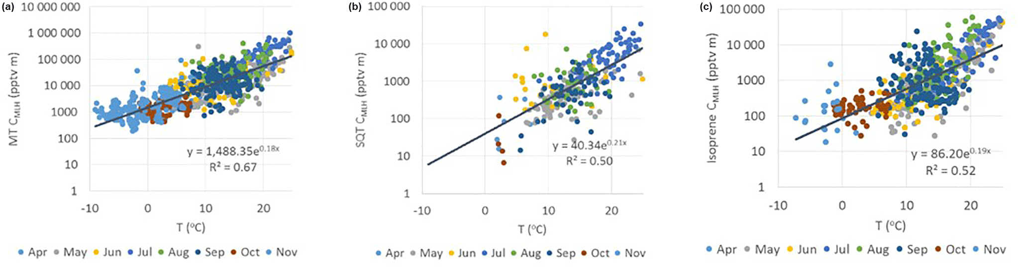
Figure 7Correlation of temperature with (a) MT, (b) SQT and (c) isoprene concentrations multiplied by the mixing layer height (CMLH) measured at the SMEAR II station in 2016. Note that the y axes are in a logarithmic scale.
Even though the VOAs were less correlated with temperature than terpenes (Table 3), the dependence of temperature sensitivity on vapour pressures was also found for all other VOAs, except butanoic acid, which was expected to be produced from the 1-butanol used in other instruments at the site. For C5–C10 aldehydes, only monthly means showed this dependence. The summertime daily means of aldehydes were more highly correlated with temperature, but β values still did not follow the vapour pressures.
These dependencies can be used to estimate the type of compound that could explain the missing reactivity found by total reactivity measurements or to assist in the identification of compounds in direct mass spectrometric methods.
3.2.8 Simple proxies for estimating local biogenic volatile organic compound concentrations
Kontkanen et al. (2016) developed MT proxies that are used for calculating concentrations of the MT sum at SMEAR II. The proxies are based on the temperature-controlled emissions from the forest ecosystem, the dilution caused by mixing within the boundary layer and various oxidation processes. Our data show that the monthly and daily means of both the sum and individual MTs and most other BVOC concentrations can be described relatively well, using only the temperature (Tables 3 and 4, Fig. 5), and a simplified proxy for the daily or monthly mean concentrations would be
where α and β are empirical coefficients found in Table 3 and obtained from the correlation of monthly and daily mean concentrations with temperature (Fig. 5) and T is the ambient temperature.
However, describing the diurnal variation in mixing of air must be taken into account. To roughly describe the dilution caused by the vertical mixing we multiplied the concentrations with the MLHs (CMLH= [VOC] × MLH) and studied the correlation of these CMLH values with temperature (Table 3 and Fig. 7). All individual measured data points available from the year 2016 were used, except the cases in which MLH was below the detection limit of the lidar (<60 m). Therefore, the highest values during the most stable nights are missing. The correlation of the CMLH values with temperature was best for the MTs (). The modelling study of Zhou et al. (2017) showed that the variation in MT concentrations was mainly driven by the emissions and mixing, while for faster-reacting SQTs oxidation also plays a role. For oxygenated compounds production in the atmosphere and deposition also affect local concentrations, and therefore correlation of the CMLH values with temperature was lower than for the MTs (Table 3). In our case the proxy for the concentration of the MT or SQT sum or an individual compound (BVOCi), when MLH >60 m, would be
where α and β are empirical coefficients found in Table 3 and obtained from the correlation of concentrations multiplied by the MLH (CMLH) with temperature (Fig. 7), T is the ambient temperature and MLH is the mixing layer height.
3.3 Importance of studied the biogenic volatile organic compounds for local atmospheric chemistry
3.3.1 Reactivity of the measured biogenic volatile organic compounds
To describe the effects of various compounds and compound groups on the oxidation capacity of the atmosphere, we calculated the OH, NO3 and O3 reactivities for the BVOCs studied using the measured concentrations and reaction rates with different oxidants (Eq. 4). The OH reactivity of the MTs was clearly higher than for any other VOC group at this boreal forest site, showing the importance of the MTs for local OH chemistry (Fig. 8a). The OH reactivity of the MTs was 10 times higher than for SQTs, even in July when the SQT concentrations were highest. The OH reactivity of the other compound groups were minor (approximately 4 % in July). Based on additional measurements in July, the contribution of carbonyls <C5 (formaldehyde, acetaldehyde, acetone and butanal) was minor. However, even when reactivities of all the BVOCs, anthropogenic VOCs and other OH-reactive compounds measured at the site were added up, the OH reactivity was much lower (<50 %) than the total reactivity measured at the site by Sinha et al. (2010), Nölscher et al. (2012) and Praplan et al. (2018). In a previous modelling study at the site, the OH reactivity of the MTs was also highest, but the other VOCs showed almost as high a contribution (Mogensen et al., 2011). These other VOCs included 415 compounds mainly consisting of second- or higher-order organic reaction products, but not SQTs. Even with these reaction products, approximately 50–70 % of the measured total OH reactivity remained unexplained.
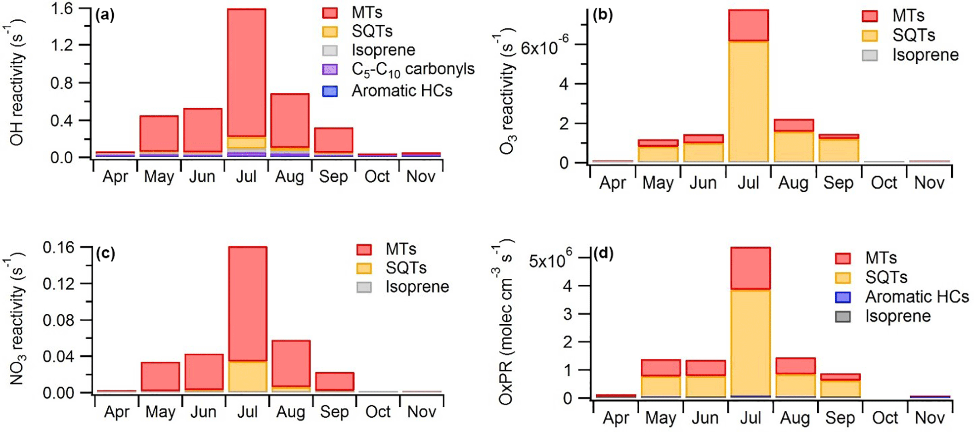
Figure 8(a) Hydroxyl (OH) reactivity, (b) ozone (O3) reactivity, (c) nitrate (NO3) reactivity and (d) production rates of oxidation products (OxPRs) of different VOC groups at SMEAR II during different months in 2016. MTs: monoterpenes, SQTs: sesquiterpenes, HCs: hydrocarbons.
Since O3 reacted only with unsaturated VOCs, only isoprene, most MTs, SQTs and unsaturated alcohols of the measured VOCs contributed to the O3 reactivity. From May to September, the SQTs contributed greatly to the O3 reactivity (Fig. 8b). Even though the MT concentrations were approximately 50 times higher than the SQT concentrations, the O3 reactivity of SQTs was about 3 times higher than that of the MTs. Hakola et al. (2017) also showed the crucial importance of the SQTs for the O3 reactivity in the spruce emissions. This indicates that the SQTs, especially β-caryophyllene (Fig. S8d), have much higher effects on local O3 destruction than MTs. Several studies have shown that the O3 deposition fluxes measured cannot be explained by stomatal and known non-stomatal sinks modelled, such as reactions with the VOCs measured in the gas phase (Wolfe et al., 2011; Rannik et al., 2012; Clifton et al., 2017). The higher-than-expected impact of the SQTs could explain at least part of the discrepancy.
The NO3 radicals also mainly reacted with the unsaturated VOCs, and the MTs clearly contributed most to the NO3 reactivity of BVOCs at the site (Fig. 8c). Of the SQTs only β-caryophyllene was considered, since the reaction rate coefficients were not available for the others. However, β-caryophyllene showed the highest concentrations of all the SQTs, but still did not significantly affect the NO3 reactivity. Liebmann et al. (2018) measured the total NO3 reactivity at the site in September 2016, and the BVOCs measured at the same time explained 70 % of the reactivity during the night but only 40 % during the day.
α-Pinene contributed most to the OH, O3 and NO3 reactivities, similar to the concentrations of the individual MTs (Fig. S8). However, limonene and terpinolene both have relatively fast rate coefficients with the OH radicals and O3; therefore, despite being present at lower concentrations, they can greatly impact the formation of secondary products. In addition, limonene shows a higher SOA yield than MTs generally (Lee et al., 2006) and, therefore, it was expected to be more important for SOA production than the concentrations indicate. Of the individual SQTs β-caryophyllene played a major role in contributing OH reactivity, while for the O3 reactivity it contributed the most (>60 % in June–August) of all the VOCs measured (Fig. S8).
3.3.2 Oxidation products and secondary organic aerosols
Oxidation of VOCs, under various environmental conditions, produces a variety of gas- and particle-phase products that are relevant for atmospheric chemistry and SOA production. To describe this we calculated OxPRs from the isoprene, MT, SQT and OVOC reactions as described in Sect. 2.5.
More oxidation products were produced from SQTs than from MTs (Fig. 8d). The contribution of OVOCs, aromatic hydrocarbons and isoprene was very low. SQTs were very important especially during summer nights (Figs. 8 and 9). The daytime contributions of MTs and SQTs were similar during all months except in July when the SQTs predominated even in midday. In addition, photooxidation of SQTs in smog-chamber experiments generally resulted in much greater aerosol yields than MTs (Hoffmann et al., 1996; Griffin et al., 1999; Lee et al., 2006) and, therefore, they were expected to strongly influence SOA production. However, these OxPRs described very local situations and even though the rapid reactions of SQTs showed very strong local effects MTs also reacted relatively rapidly, producing secondary products on a regional scale. The global emissions of SQTs may be about 20 % of the MT emissions (Guenther et al., 2012), but this is probably a low-end estimate, since evidence for additional unaccounted SQTs and their oxidation products clearly exists (Yee et al., 2018).

Figure 9Diurnal variations in production rates for secondary organic compounds (OxPRs) from the reactions of (a) monoterpenes (MTs) and (b) sesquiterpenes (SQTs) with different oxidants (hydroxyl radical, OH; ozone, O3; and nitrate radical, NO3) and (c) contribution of individual biogenic volatile organic compounds (BVOCs) to the total OxPR during different months. The NO3 radical reactions are missing for October, since the data for calculating its proxy were not available.
α-Pinene is often used as a proxy for all BVOCs, but as shown in Fig. 9, the contribution of α-pinene to the total oxidation reactions was relatively low (approximately 20 %). The most important individual reaction generating oxidation products at the site was the reaction of β-caryophyllene with O3. For SQTs the contributions of the OH and NO3 reactions were very low, especially during the summer months (<2 %). For MTs, the O3 reactions were also the most important, while the OH radicals contributed about 30 % during summer days and the NO3 reactions were important at night. Peräkylä et al. (2014) stated that for MTs, nighttime oxidation is dominated by the NO3 radicals whereas daytime oxidation is dominated by O3. However, as in our study, O3 also predominated during summer nights. If we account for emissions and concentrations also being highest during summer, O3 becomes the most important oxidant for the production of oxidation products of MTs at night as well. For SQTs, O3 oxidation clearly dominates the first step of the reactions. However, the reaction products of MTs and SQTs, which have lost all their double bonds, continued to react with OH and NO3 and their total contribution was expected to be higher. At nighttime reaction products of MTs may build up in the atmosphere and are oxidised after sunrise with OH radicals, promoting particle growth (Peräkylä et al., 2014). Our results suggest that this also applies for SQTs.
We measured an exceptionally large dataset of VOCs in boreal forest, including terpenoid compounds (isoprene, MTs, SQTs), aldehydes, alcohols and organic acids during 26 months over a 3-year period. The measurements revealed that, of the terpenoids, MTs showed the highest concentrations at the site, but we were also able to measure highly reactive SQTs, such as β-caryophyllene and other SQTs in the ambient air, due to the availability of an instrument with improved sensitivity. Our results indicate that, in addition to terpenoids, most of the VOAs, aldehydes and alcohols have a biogenic origin either from direct emissions or by production from the other BVOCs in the atmosphere through oxidation reactions.
Temperature was the major factor controlling the concentrations of BVOCs in the air of a boreal forest. Both monthly and daily mean concentrations of MTs showed very strong exponential correlation with temperature ( and ). The SQT concentrations were even more strongly correlated with temperature and showed higher temperature sensitivity than the MTs, especially monthly mean concentrations in 2016 (R2=0.97). The results also indicate that, in spring and even more in autumn, sources (e.g. needle and leaf litter) other than temperature-dependent emissions from the main local trees greatly impact MT and SQT concentrations.
The temperature sensitivities of the most abundant terpenoids, aldehydes and VOAs within the same class of compounds were dependent on vapour pressures. This knowledge can be used to characterize the missing reactivity found in forests during total reactivity studies (Yang et al., 2016) and to aid in identification of the masses in direct mass spectrometric measurements of BVOCs and their reaction products.
We also evaluated the effect that different BVOCs have on the local atmospheric chemistry, although the MTs dominated the OH and NO3 radical chemistry. Due to the very rapid rate coefficient of O3 with SQTs, a relatively small concentration (50 times lower than MTs) of SQTs can greatly impact O3 deposition. The SQTs also generated more oxidation products than the MTs. Since the products of SQTs are also less volatile than the MT oxidation products, SQTs were expected to have even higher impact on local SOA production. Both MT and SQT oxidation was dominated by O3 especially during summer. Oxidation of other VOC groups showed very minor contributions to the formation of oxidation products at the site. Our results clearly indicate that SQTs must be considered in local SOA studies, e.g. in interpreting the results from direct mass spectrometric measurements or modelling SOA formation and growth.
GC-MS and lidar data used in this work are available from the authors upon request (heidi.hellen@fmi.fi). Trace gas and meteorological data are available at the SmartSmear AVAA portal (Junninen et al., 2009; http://avaa.tdata.fi/web/smart/smear/download, last access: 27 September 2018).
The supplement related to this article is available online at: https://doi.org/10.5194/acp-18-13839-2018-supplement.
HeH designed and conducted the VOC measurements, performed the data analysis and led the writing of the manuscript. HaH supervised the study, helped design the measurement campaign and the commented on the manuscript. APP helped conduct the measurement campaign and data analysis and commented on the manuscript. TT assisted in the GC-MS measurements and data analysis and commented on the manuscript. IY provided the aerosol surface area data, wrote their description and commented on the manuscript. VV provided the mixing layer height data, wrote their description and commented on the manuscript. JB, TP and MK provided the infrastructure at the SMEAR III site, provided additional data and commented on the manuscript.
The authors declare that they have no conflict of interest.
The research was supported by the Academy of Finland via the Academy Research
Fellow project (Academy of Finland, project 275608) and the Center of
Excellence in Atmospheric Sciences (grant no. 307331). The data providers of
the SmartSmear AVAA portal are gratefully acknowledged.
Edited by: Astrid Kiendler-Scharr
Reviewed by: three anonymous referees
Aalto, J., Kolari, P., Hari, P., Kerminen, V.-M., Schiestl-Aalto, P., Aaltonen, H., Levula, J., Siivola, E., Kulmala, M., and Bäck, J.: New foliage growth is a significant, unaccounted source for volatiles in boreal evergreen forests, Biogeosciences, 11, 1331–1344, https://doi.org/10.5194/bg-11-1331-2014, 2014.
Aalto, P., Hämeri, K., Becker, E. D. O., Weber, R., Salm, J., Mäkelä, J. M., Hoell, C., O'dowd, C. D., Hansson, H.-C., Väkevä, M., Koponen, I. K., Buzorius, G., and Kulmala, M.: Physical characterization of aerosol particles during nucleation events, Tellus B, 53, 344–358, 2001.
Aaltonen, H., Pumpanen, J., Pihlatie, M., Hakola, H., Hellén, H., Kulmala, L., Vesala, T., and Bäck, J.: Boreal pine forest floor biogenic volatile organic compound emissions peak in early summer and autumn, Agr. Forest Meteorol., 151, 682–691, https://doi.org/10.1016/j.agrformet.2010.12.010, 2011.
Atkinson, R.: Gas-phase tropospheric chemistry of organic compounds, J. Phys. Chem. Ref. Data, 2, 216 pp., 1994.
Bäck, J., Aalto, J., Henriksson, M., Hakola, H., He, Q., and Boy, M.: Chemodiversity of a Scots pine stand and implications for terpene air concentrations, Biogeosciences, 9, 689–702, https://doi.org/10.5194/bg-9-689-2012, 2012.
Biesenthal, T. A. and Shepson, P. B.: Observations of anthropogenic inputs of the isoprene oxidation products methyl vinyl hetone and methacrolein to teh atmosphere, Geophys. Res. Lett., 24, 1375–1378, 1997.
Blande, J. D., Turunen, K., and Holopainen, J. K.: Pine weevil feeding on Norway spruce bark has a stronger impact on needle VOC emissions than enhanced ultraviolet-B radiation, Environ. Pollut., 157, 174–180, 2009.
Bourtsoukidis, E., Behrendt, T., Yañez-Serrano, A. M., Hellén, H., Diamantopoulos, E., Catão, E., Ashworth, K., Pozzer, A., Quesada, C. A., Martins, D. L., Sá, M., Araujo, A., Brito, J., Artaxo, P., Kesselmeier, J., Lelieveld, J., and Williams, J.: Strong sesquiterpene emissions from Amazonian soils, Nat. Commun., 9, 2226, https://doi.org/10.1038/s41467-018-04658-y, 2018.
Bouvier-Brown, N. C., Goldstein, A. H., Gilman, J. B., Kuster, W. C., and de Gouw, J. A.: In-situ ambient quantification of monoterpenes, sesquiterpenes, and related oxygenated compounds during BEARPEX 2007: implications for gas- and particle-phase chemistry, Atmos. Chem. Phys., 9, 5505–5518, https://doi.org/10.5194/acp-9-5505-2009, 2009.
Bowman, J. H., Barket, D. J., and Shepson, P. B.: Atmospheric chemistry of nonanal, Environ. Sci. Technol., 37, 2218–2225, 2003.
Calvert, J. G., Mellouki, A., and Orlando, J. J.: The mechanism of atmospheric oxidation of the oxygenates, Oxford University Press, New York, 2011.
Ciccioli, P. and Mannozzi, M.: High-Molecular-Weight Carbonyls and Carboxylic Acids in Volatile organic compounds in the atmosphere, edited by: Koppmann R., Blackwell Publishing Ltd, 292–341, https://doi.org/10.1002/9780470988657.ch8, 2007.
Clifton, O. E., Fiore, A. M., Munger, J. W., Malyshev, S., Horowitz, L. W., Shevliakova, E., Paulot, F., Murray, L. T., and Griffin, K. L.: Interannual variability in ozone removal by a temperate deciduous forest, Geophys. Res. Lett., 44, 542–552, https://doi.org/10.1002/2016GL070923, 2017.
Duhl, T. R., Helmig, D., and Guenther, A.: Sesquiterpene emissions from vegetation: a review, Biogeosciences, 5, 761–777, https://doi.org/10.5194/bg-5-761-2008, 2008.
Eerdekens, G., Yassaa, N., Sinha, V., Aalto, P. P., Aufmhoff, H., Arnold, F., Fiedler, V., Kulmala, M., and Williams, J.: VOC measurements within a boreal forest during spring 2005: on the occurrence of elevated monoterpene concentrations during night time intense particle concentration events, Atmos. Chem. Phys., 9, 8331–8350, https://doi.org/10.5194/acp-9-8331-2009, 2009.
Fall, R.: Biogenic emissions of volatile organic compounds from higher plants, in: Reactive Hydrocarbons in the Atmosphere, edited by: Hewitt, C. N., San Diego, Academic Press, 43–96, 1999.
Ghirardo, A., Koch, K., Taipale, R., Zimmer, I., Schnitzler, J.-P., and Rinne, J.: Determination of de novo and pool emissions of terpenes from four common boreal/alpine trees by 13CO2 labelling and PTR-MS analysis, Plant Cell Environ., 33, 781–792, https://doi.org/10.1111/j.1365-3040.2009.02104.x, 2010.
Glasius, M. and Goldstein, A.: Recent discoveries and future challenges in atmospheric organic chemistry, Environ. Sci. Technol., 50, 2754–2764, 2016.
Griffin, R. J., Cocker III, D. R., Flagan, R. C., and Seinfeld, J. H.: Organic aerosol formation from the oxidation of biogenic hydrocarbons, J. Geophys. Res., 104, 3555–3567, 1999.
Grosjean, D., Williams, E. L., Grosjean, E., Andino, J. M., and Seinfeld, J. H.: Atmospheric oxidation of biogenic hydrocarbons: Reaction of ozone with β- pinene, D-limonene and trans-caryophyllene, Environ. Sci. Technol., 27, 2754–2758, https://doi.org/10.1021/es00049a014, 1993.
Guenther, A. B., Zimmerman, P. R., Harley, P. C., Monson, R. K., and Fall, R.: Isoprene and monoterpene emission rate variability: Model evaluation and sensitivity analyses, J. Geophys. Res., 98, 12609–12627, 1993.
Guenther, A. B., Jiang, X., Heald, C. L., Sakulyanontvittaya, T., Duhl, T., Emmons, L. K., and Wang, X.: The Model of Emissions of Gases and Aerosols from Nature version 2.1 (MEGAN2.1): an extended and updated framework for modeling biogenic emissions, Geosci. Model Dev., 5, 1471–1492, https://doi.org/10.5194/gmd-5-1471-2012, 2012.
Hakola, H., Arey, J., Aschmann, S. M., and Atkinson, R.: Product formation from the gas-phase reactions of OH radicals and O3 with a series of monoterpenes, J. Atmos. Chem., 18, 75–102, 1994.
Hakola, H., Rinne, J., and Laurila, T.: The hydrocarbon emission rates of Tea-Leaved Willow (Salix phylicifolia), Silver Birch (Betula pendula) and European Aspen (Populus tremula), Atmos. Environ., 32, 1825–1833, 1998.
Hakola, H., Laurila, T., Lindfors, V., Hellén, H., Gaman, A., and Rinne, J.: Variation of the VOC emission rates of birch species during the growing season, Boreal Environ. Res., 6, 237–249, 2001.
Hakola, H., Tarvainen, V., Laurila, T., Hiltunen, V., Hellén, H., and Keronen, P.: Seasonal variation of VOC concentrations above a boreal coniferous forest, Atmos. Environ., 37, 1623–1634, 2003.
Hakola, H., Tarvainen, V., Bäck, J., Ranta, H., Bonn, B., Rinne, J., and Kulmala, M.: Seasonal variation of mono- and sesquiterpene emission rates of Scots pine, Biogeosciences, 3, 93–101, https://doi.org/10.5194/bg-3-93-2006, 2006.
Hakola, H., Hellén, H., Tarvainen, V., Bäck, J., Patokoski, J., and Rinne, J.: Annual variations of atmospheric VOC concentrations in a boreal forest, Boreal Environ. Res., 14, 722–730, 2009.
Hakola, H., Hellén, H., Hemmilä, M., Rinne, J., and Kulmala, M.: In situ measurements of volatile organic compounds in a boreal forest, Atmos. Chem. Phys., 12, 11665–11678, https://doi.org/10.5194/acp-12-11665-2012, 2012.
Hakola, H., Tarvainen, V., Praplan, A. P., Jaars, K., Hemmilä, M., Kulmala, M., Bäck, J., and Hellén, H.: Terpenoid and carbonyl emissions from Norway spruce in Finland during the growing season, Atmos. Chem. Phys., 17, 3357–3370, https://doi.org/10.5194/acp-17-3357-2017, 2017.
Hari, P. and Kulmala, M.: Station for measuring ecosystem-atmosphere relations (SMEAR II), Boreal Environ. Res., 10, 315–322, 2005.
Hellén, H., Hakola, H., Reissell, A., and Ruuskanen, T. M.: Carbonyl compounds in boreal coniferous forest air in Hyytiälä, Southern Finland, Atmos. Chem. Phys., 4, 1771–1780, https://doi.org/10.5194/acp-4-1771-2004, 2004.
Hellén, H., Hakola, H., Pystynen, K.-H., Rinne, J., and Haapanala, S.: C2-C10 hydrocarbon emissions from a boreal wetland and forest floor, Biogeosciences, 3, 167–174, https://doi.org/10.5194/bg-3-167-2006, 2006.
Hellén, H., Kuronen, P., and Hakola, H.: Heated stainless steel tube for ozone removal in the ambient air measurements of mono- and sesquiterpenes, Atmos. Environ., 57, 35–40, 2012.
Hellén, H., Schallhart, S., Praplan, A. P., Petäjä, T., and Hakola, H.: Using in situ GC-MS for analysis of C2–C7 volatile organic acids in ambient air of a boreal forest site, Atmos. Meas. Tech., 10, 281–289, https://doi.org/10.5194/amt-10-281-2017, 2017.
Hens, K., Novelli, A., Martinez, M., Auld, J., Axinte, R., Bohn, B., Fischer, H., Keronen, P., Kubistin, D., Nölscher, A. C., Oswald, R., Paasonen, P., Petäjä, T., Regelin, E., Sander, R., Sinha, V., Sipilä, M., Taraborrelli, D., Tatum Ernest, C., Williams, J., Lelieveld, J., and Harder, H.: Observation and modelling of HOx radicals in a boreal forest, Atmos. Chem. Phys., 14, 8723–8747, https://doi.org/10.5194/acp-14-8723-2014, 2014.
Hoffmann, T., Odum, J., Bowman, F., Collins, D., Klockow, D., Flagan, R. C., and Seinfeld, J. H.: Aerosol formation potential of biogenic hydrocarbons, J. Aerosol Sci., 27, S233–S234, 1996.
Holopainen, J.: Multiple functions of inducible plant volatiles, Trends Plant Sci., 9, 529–533, 2004.
Ilvesniemi, H., Levula, J., Ojansuu, R., Kolari, P., Kulmala, L., Pumpanen, J., Launiainen, S., Vesala, T., and Nikinmaa, E.: Long-term measurements of the carbon balance of a boreal Scots pine dominated forest ecosystem, Boreal Environ. Res., 14, 731–753, 2009.
Jardine, A. B., Jardine, K. J., Fuentes, J. D., Martin, S. T., Martins, G., Durgante, F., Carneiro, V., Higuchi, N., Manzi, A. O., and Chambers, J. Q.: Highly reactive light-dependent monoterpenes in the Amazon, Geophys. Res. Lett., 42, 1576–1583, https://doi.org/10.1002/2014GL062573, 2015.
Jardine, K., Yanez Serrano, A., Arneth, A., Abrell, L., Jardine, A., van Haren, J., Artaxo P., Rizzo, L. V., Ishilda, F. Y., Karl, T., Kesselmeier, J., Saleska, S., and Huxman, T.: Within-canopy sesquiterpene ozonolysis in Amazonia, J. Geophys. Res., 116, D19301, https://doi.org/10.1029/2011JD016243, 2011.
Jones, C. E., Hopkins, J. R., and Lewis, A. C.: In situ measurements of isoprene and monoterpenes within a south-east Asian tropical rainforest, Atmos. Chem. Phys., 11, 6971–6984, https://doi.org/10.5194/acp-11-6971-2011, 2011.
Junninen, H., Lauri, A., Keronen, P., Aalto, P., Hiltunen, V., Hari, P., and Kulmala, M.: Smart-SMEAR: on-line data exploration and visualization tool for SMEAR stations, Boreal Environ. Res., 14, 447–457, 2009.
Kaminski, M., Fuchs, H., Acir, I.-H., Bohn, B., Brauers, T., Dorn, H.-P., Häseler, R., Hofzumahaus, A., Li, X., Lutz, A., Nehr, S., Rohrer, F., Tillmann, R., Vereecken, L., Wegener, R., and Wahner, A.: Investigation of the β-pinene photooxidation by OH in the atmosphere simulation chamber SAPHIR, Atmos. Chem. Phys., 17, 6631–6650, https://doi.org/10.5194/acp-17-6631-2017, 2017.
Kännaste, A., Nordenhem, H., Nordlander, G., and Borg-Karlson, A.-K.: Volatiles from a Mite-Infested Spruce Clone and their Effects on PineWeevil Behavior, J. Chem. Ecol., 35, 1262–1271, 2009.
Kesselmeier, J., Kuhn, U., Rottenberger, S., Biesenthal, T., Wolf, A., Schebeske, G., Andreae, M. O., Ciccioli, P., Brancaleoni, E., Frattoni, M., Oliva, S. T., Botelho, M. L., Silva, C. M. A., and Tavares, T. M.: Concentrations and species composition of atmospheric volatile organic compounds (VOCs) as observed during the wet and dry season in Rondônia (Amazonia), J. Geophys. Res., 107, 8053, https://doi.org/10.1029/2000JD000267, 2002.
Kim, S., Karl, T., Helmig, D., Daly, R., Rasmussen, R., and Guenther, A.: Measurement of atmospheric sesquiterpenes by proton transfer reaction-mass spectrometry (PTR-MS), Atmos. Meas. Tech., 2, 99–112, https://doi.org/10.5194/amt-2-99-2009, 2009.
Kim, S., Karl, T., Guenther, A., Tyndall, G., Orlando, J., Harley, P., Rasmussen, R., and Apel, E.: Emissions and ambient distributions of Biogenic Volatile Organic Compounds (BVOC) in a ponderosa pine ecosystem: interpretation of PTR-MS mass spectra, Atmos. Chem. Phys., 10, 1759–1771, https://doi.org/10.5194/acp-10-1759-2010, 2010.
Kontkanen, J., Paasonen, P., Aalto, J., Bäck, J., Rantala, P., Petäjä, T., and Kulmala, M.: Simple proxies for estimating the concentrations of monoterpenes and their oxidation products at a boreal forest site, Atmos. Chem. Phys., 16, 13291–13307, https://doi.org/10.5194/acp-16-13291-2016, 2016.
Kulmala, M., Kontkanen, J., Junninen, H., Lehtipalo, K., Manninen, H. E., Nieminen, T., Petaja, T., Sipila, M., Schobesberger, S., Rantala, P., Franchin, A., Jokinen, T., Jarvinen, E., Aijala, M., Kangasluoma, J., Hakala, J., Aalto, P. P., Paasonen, P., Mikkila,J., Vanhanen, J., Aalto, J., Hakola, H., Makkonen, U., Ruuskanen, T., Mauldin, R. L., Duplissy, J., Vehkamaki, H., Back, J., Kortelainen, A., Riipinen, I., Kurten, T., Johnston, M. V., Smith, J. N., Ehn, M., Mentel, T. F., Lehtinen, K. E. J., Laaksonen, A., Kerminen, V. M., and Worsnop, D. R.: Direct observations of atmospheric aerosol nucleation, Science, 339, 943–946, https://doi.org/10.1126/science.1227385, 2013.
Lappalainen, H. K., Sevanto, S., Bäck, J., Ruuskanen, T. M., Kolari, P., Taipale, R., Rinne, J., Kulmala, M., and Hari, P.: Day-time concentrations of biogenic volatile organic compounds in a boreal forest canopy and their relation to environmental and biological factors, Atmos. Chem. Phys., 9, 5447–5459, https://doi.org/10.5194/acp-9-5447-2009, 2009.
Lee, A., Goldstein, A. H., Kroll, J. H., Ng, N. L., Varutbangkul, V., Flagan, R. C., and Seinfeld, J. H.: Gas-phase products and secondary aerosol yields from the photooxidation of 16 different terpenes, J. Geophys. Res., 111, D17305, https://doi.org/10.1029/2006JD007050, 2006.
Liao, L., Dal Maso, M., Taipale, R., Rinne, J., Ehn, M., Junninen, H., Äijälä, M., Nieminen, T., Alekseychik, P., Hulkkonen, M., Worsnop, D. R., Kerminen, V.-M., and Kulmala, M.: Monoterpene pollution episodes in a forest environment: indication of anthropogenic origin and association with aerosol particles, Boreal Environ. Res., 16, 288–303, 2011.
Liebmann, J., Karu, E., Sobanski, N., Schuladen, J., Ehn, M., Schallhart, S., Quéléver, L., Hellen, H., Hakola, H., Hoffmann, T., Williams, J., Fischer, H., Lelieveld, J., and Crowley, J. N.: Direct measurement of NO3 radical reactivity in a boreal forest, Atmos. Chem. Phys., 18, 3799–3815, https://doi.org/10.5194/acp-18-3799-2018, 2018.
Mäki, M., Heinonsalo, J., Hellén, H., and Bäck, J.: Contribution of understorey vegetation and soil processes to boreal forest isoprenoid exchange, Biogeosciences, 14, 1055–1073, https://doi.org/10.5194/bg-14-1055-2017, 2017.
Manninen, A. J., O'Connor, E. J., Vakkari, V., and Petäjä, T.: A generalised background correction algorithm for a Halo Doppler lidar and its application to data from Finland, Atmos. Meas. Tech., 9, 817–827, https://doi.org/10.5194/amt-9-817-2016, 2016.
Mellouki, A., Wallington, T. J., and Chen, J.: Atmospheric chemistry of oxygenated volatile organic compounds: Impacts on air quality and climate, Chem. Rev., 115, 3984–4014, https://doi.org/10.1021/cr500549n, 2015.
Mogensen, D., Smolander, S., Sogachev, A., Zhou, L., Sinha, V., Guenther, A., Williams, J., Nieminen, T., Kajos, M. K., Rinne, J., Kulmala, M., and Boy, M.: Modelling atmospheric OH-reactivity in a boreal forest ecosystem, Atmos. Chem. Phys., 11, 9709–9719, https://doi.org/10.5194/acp-11-9709-2011, 2011.
Ng, N. L., Brown, S. S., Archibald, A. T., Atlas, E., Cohen, R. C., Crowley, J. N., Day, D. A., Donahue, N. M., Fry, J. L., Fuchs, H., Griffin, R. J., Guzman, M. I., Herrmann, H., Hodzic, A., Iinuma, Y., Jimenez, J. L., Kiendler-Scharr, A., Lee, B. H., Luecken, D. J., Mao, J., McLaren, R., Mutzel, A., Osthoff, H. D., Ouyang, B., Picquet-Varrault, B., Platt, U., Pye, H. O. T., Rudich, Y., Schwantes, R. H., Shiraiwa, M., Stutz, J., Thornton, J. A., Tilgner, A., Williams, B. J., and Zaveri, R. A.: Nitrate radicals and biogenic volatile organic compounds: oxidation, mechanisms, and organic aerosol, Atmos. Chem. Phys., 17, 2103–2162, https://doi.org/10.5194/acp-17-2103-2017, 2017.
Nölscher, A. C., Williams, J., Sinha, V., Custer, T., Song, W., Johnson, A. M., Axinte, R., Bozem, H., Fischer, H., Pouvesle, N., Phillips, G., Crowley, J. N., Rantala, P., Rinne, J., Kulmala, M., Gonzales, D., Valverde-Canossa, J., Vogel, A., Hoffmann, T., Ouwersloot, H. G., Vilà-Guerau de Arellano, J., and Lelieveld, J.: Summertime total OH reactivity measurements from boreal forest during HUMPPA-COPEC 2010, Atmos. Chem. Phys., 12, 8257–8270, https://doi.org/10.5194/acp-12-8257-2012, 2012.
O'Connor, E. J., Illingworth, A. J., Brooks, I. M., Westbrook, C. D., Hogan, R. J., Davies, F., and Brooks, B. J.: A Method for Estimating the Turbulent Kinetic Energy Dissipation Rate from a Vertically Pointing Doppler Lidar, and Independent Evaluation from Balloon-Borne In Situ Measurements, J. Atmos. Ocean. Tech., 27, 1652–1664, https://doi.org/10.1175/2010JTECHA1455.1, 2010.
Paulson, S. E., Flagan, R. C., and Seinfeld, J. H.: Atmospheric photooxidation of isoprene, 2, The ozone-isoprene reaction, Int. J. Chem. Kinet., 24, 103–125, 1992.
Pearson, G., Davies, F., and Collier, C.: An Analysis of the Performance of the UFAM Pulsed Doppler Lidar for Observing the Boundary Layer, J. Atmos. Ocean. Tech., 26, 240–250, https://doi.org/10.1175/2008JTECHA1128.1, 2009.
Peräkylä, O., Vogt, M., Tikkanen, O.-P., Laurila, T., Kajos, M. K., Rantala, P. A., Patokoski, J., Aalto, J., Yli-Juuti, T., Ehn, M., Sipilä, M., Paasonen, P., Rissanen, M., Nieminen, T., Taipale, R., Keronen, P., Lappalainen, H. K., Ruuskanen, T. M., Rinne, J., Kerminen, V.-M., Kulmala, M., Bäck, J., and Petäjä, T.: Monoterpenes' oxidation capacity and rate over a boreal forest: temporal variation and connection to growth of newly formed particles, Boreal Environ. Res., 19, 293–310, 2014.
Petäjä, T., Mauldin, III, R. L., Kosciuch, E., McGrath, J., Nieminen, T., Paasonen, P., Boy, M., Adamov, A., Kotiaho, T., and Kulmala, M.: Sulfuric acid and OH concentrations in a boreal forest site, Atmos. Chem. Phys., 9, 7435–7448, https://doi.org/10.5194/acp-9-7435-2009, 2009.
Petterson, M.: Stress related emissions of Norway spruce plants, Licentiate thesis, KTH Royal Institute of technology, Stockholm, ISBN-13: 978-91-7178-644-9, 2007.
Possanzini, M., Di Palo, V., Brancaleoni, E., Frattoni, M., and Ciccioli, P.: A train of carbon and DNPH-coated catridges for the determination of carbonyls from C1 to C12 in air and emission samples, Atmos. Environ., 34, 5311-2318, 2000.
Praplan, A. P., Pfannerstill, E. Y., Williams, J., and Hellén, H.: OH reactivity of the urban air in Helsinki, Finland, during winter, Atmos. Environ., 169, 150–161, https://doi.org/10.1016/j.atmosenv.2017.09.013, 2017.
Praplan, A. P., Tykkä, T., Boy, M., Taipale D., Vakkari V. and Hellén, H.: Long-term total OH reactivity measurements in a boreal forest, in preparation, 2018.
Rannik, Ü., Altimir, N., Mammarella, I., Bäck, J., Rinne, J., Ruuskanen, T. M., Hari, P., Vesala, T., and Kulmala, M.: Ozone deposition into a boreal forest over a decade of observations: evaluating deposition partitioning and driving variables, Atmos. Chem. Phys., 12, 12165–12182, https://doi.org/10.5194/acp-12-12165-2012, 2012.
Rivera-Rios, J. C., Nguyen, T. B., Crounse, J. D., Jud, W., St. Clair, J. M., Mikoviny, T., Gilman, J. B., Lerner, B. M., Kaiser, J. B., de Gouw, J., Wisthaler, A., Hansel, A., Wennberg, P. O., Seinfeld, J. H., and Keutsch, F. N.: Conversion of hydroperoxides to carbonyls in field and laboratory instrumentation: Observational bias in diagnosing pristine versus anthropogenically controlled atmospheric chemistry, Geophys. Res. Lett., 41, 8645–8651, https://doi.org/10.1002/2014GL061919, 2014.
Rohrer, F. and Berresheim, H.: Strong correlation between levels of tropospheric hydroxyl radicals and solar ultraviolet radiation, Nature, 442, 184–187, https://doi.org/10.1038/nature04924, 2006.
Seco, R., Penuelas, J., and Filella, I.: Short-chain oxygenated VOCs: Emission and uptake by plants and atmospheric sources, sinks, and concentrations, Atmos. Environ., 41, 2477–2499, 2007.
Scala, A., Allmann, S., Mirabella, R., Haring, M. A., and Schuurink, R. C.: Green leaf volatiles: A Plant's multifunctional weapon against herbivores and pathogens, Int. J. Mol. Sci., 14, 17781–17811, https://doi.org/10.3390/ijms140917781, 2013.
Schallhart, S., Rantala, P., Kajos, M. K., Aalto, J., Mammarella, I., Ruuskanen, T. M., and Kulmala, M.: Temporal variation of VOC fluxes measured with PTR-TOF above a boreal forest, Atmos. Chem. Phys., 18, 815–832, https://doi.org/10.5194/acp-18-815-2018, 2018.
Sindelarova, K., Granier, C., Bouarar, I., Guenther, A., Tilmes, S., Stavrakou, T., Müller, J.-F., Kuhn, U., Stefani, P., and Knorr, W.: Global data set of biogenic VOC emissions calculated by the MEGAN model over the last 30 years, Atmos. Chem. Phys., 14, 9317–9341, https://doi.org/10.5194/acp-14-9317-2014, 2014.
Sinha, V., Williams, J., Lelieveld, J., Ruuskanen, T., Kajos, M., Patokoski, J., Hellen, H., Hakola, H., Mogensen, D., Boy, M., Rinne, J., and Kulmala, M.: OH Reactivity Measurements within a Boreal Forest: Evidence for Unknown Reactive Emissions, Environ. Sci. Technol., 44, 6614–6620, https://doi.org/10.1021/es101780b, 2010.
Tarvainen, V., Hakola, H., Hellén, H., Bäck, J., Hari, P., and Kulmala, M.: Temperature and light dependence of the VOC emissions of Scots pine, Atmos. Chem. Phys., 5, 989–998, https://doi.org/10.5194/acp-5-989-2005, 2005.
Tunved, P., Hansson, H.-C., Kerminen, V.-M., Ström, J., Dal Maso, M., Lihavainen, H., Viisanen, Y., Aalto, P. P., Komppula, M., and Kulmala, M.: High natural aerosol loading over boreal forests, Science, 312, 261–263, 2006.
Vakkari, V., O'Connor, E. J., Nisantzi, A., Mamouri, R. E., and Hadjimitsis, D. G.: Low-level mixing height detection in coastal locations with a scanning Doppler lidar, Atmos. Meas. Tech., 8, 1875–1885, https://doi.org/10.5194/amt-8-1875-2015, 2015.
Williams, J., Crowley, J., Fischer, H., Harder, H., Martinez, M., Petäjä, T., Rinne, J., Bäck, J., Boy, M., Dal Maso, M., Hakala, J., Kajos, M., Keronen, P., Rantala, P., Aalto, J., Aaltonen, H., Paatero, J., Vesala, T., Hakola, H., Levula, J., Pohja, T., Herrmann, F., Auld, J., Mesarchaki, E., Song, W., Yassaa, N., Nölscher, A., Johnson, A. M., Custer, T., Sinha, V., Thieser, J., Pouvesle, N., Taraborrelli, D., Tang, M. J., Bozem, H., Hosaynali-Beygi, Z., Axinte, R., Oswald, R., Novelli, A., Kubistin, D., Hens, K., Javed, U., Trawny, K., Breitenberger, C., Hidalgo, P. J., Ebben, C. J., Geiger, F. M., Corrigan, A. L., Russell, L. M., Ouwersloot, H. G., Vilà-Guerau de Arellano, J., Ganzeveld, L., Vogel, A., Beck, M., Bayerle, A., Kampf, C. J., Bertelmann, M., Köllner, F., Hoffmann, T., Valverde, J., González, D., Riekkola, M.-L., Kulmala, M., and Lelieveld, J.: The summertime Boreal forest field measurement intensive (HUMPPA-COPEC-2010): an overview of meteorological and chemical influences, Atmos. Chem. Phys., 11, 10599–10618, https://doi.org/10.5194/acp-11-10599-2011, 2011.
Winterhalter, R., Neeb, P., Grossmann, D., Kolloff, A., Horie, O., and Moortgat, G.: Products and Mechanism of the Gas Phase Reaction of Ozone with β-Pinene, J. Atmos. Chem., 35, 165–197, https://doi.org/10.1023/A:1006257800929, 2000.
Wolfe, G. M., Thornton, J. A., McKay, M., and Goldstein, A. H.: Forest-atmosphere exchange of ozone: sensitivity to very reactive biogenic VOC emissions and implications for in-canopy photochemistry, Atmos. Chem. Phys., 11, 7875–7891, https://doi.org/10.5194/acp-11-7875-2011, 2011.
Yáñez-Serrano, A. M., Nölscher, A. C., Bourtsoukidis, E., Gomes Alves, E., Ganzeveld, L., Bonn, B., Wolff, S., Sa, M., Yamasoe, M., Williams, J., Andreae, M. O., and Kesselmeier, J.: Monoterpene chemical speciation in a tropical rainforest:variation with season, height, and time of dayat the Amazon Tall Tower Observatory (ATTO), Atmos. Chem. Phys., 18, 3403–3418, https://doi.org/10.5194/acp-18-3403-2018, 2018.
Yang, Y., Shao, M., Wang, X., Nölscher, A. C., Kessel, S., Guenther, A., and Williams, J.: Towards a quantitative understanding of total OH reactivity: A review, Atmos. Environ., 134, 147–161, https://doi.org/10.1016/j.atmosenv.2016.03.010, 2016.
Yassaa, N., Song, W., Lelieveld, J., Vanhatalo, A., Bäck, J., and Williams, J.: Diel cycles of isoprenoids in the emissions of Norway spruce, four Scots pine chemotypes, and in Boreal forest ambient air during HUMPPA-COPEC-2010, Atmos. Chem. Phys., 12, 7215–7229, https://doi.org/10.5194/acp-12-7215-2012, 2012.
Yee, L. D., Isaacman-VanWertz, G., Wernis, R. A., Meng, M., Rivera, V., Kreisberg, N. M., Hering, S. V., Bering, M. S., Glasius, M., Upshur, M. A., Gray Bé, A., Thomson, R. J., Geiger, F. M., Offenberg, J. H., Lewandowski, M., Kourtchev, I., Kalberer, M., de Sá, S., Martin, S. T., Alexander, M. L., Palm, B. B., Hu, W., Campuzano-Jost, P., Day, D. A., Jimenez, J. L., Liu, Y., McKinney, K. A., Artaxo, P., Viegas, J., Manzi, A., Oliveira, M. B., de Souza, R., Machado, L. A. T., Longo, K., and Goldstein, A. H.: Observations of sesquiterpenes and their oxidation products in central Amazonia during the wet and dry seasons, Atmos. Chem. Phys., 18, 10433–10457, https://doi.org/10.5194/acp-18-10433-2018, 2018.
Yuan, B., Koss, A., Warneke, C., Coggob, M., Sekimoto, K., and de Gouw, L. A.: Proton-transfer-reaction mass spectrometry: Applications in Atmospheric Sciences, Chem. Rev., 117, 13187–13229, https://doi.org/10.1021/acs.chemrev.7b00325, 2017.
Zhou, P., Ganzeveld, L., Taipale, D., Rannik, Ü., Rantala, P., Rissanen, M. P., Chen, D., and Boy, M.: Boreal forest BVOC exchange: emissions versus in-canopy sinks, Atmos. Chem. Phys., 17, 14309–14332, https://doi.org/10.5194/acp-17-14309-2017, 2017.