the Creative Commons Attribution 4.0 License.
the Creative Commons Attribution 4.0 License.
 | 25 Sep 2018
Reanalysis intercomparisons of stratospheric polar processing diagnostics
Zachary D. Lawrence
Gloria L. Manney
Krzysztof Wargan
We compare herein polar processing diagnostics derived from the four most recent “full-input” reanalysis datasets: the National Centers for Environmental Prediction Climate Forecast System Reanalysis/Climate Forecast System, version 2 (CFSR/CFSv2), the European Centre for Medium-Range Weather Forecasts Interim (ERA-Interim) reanalysis, the Japanese Meteorological Agency's 55-year (JRA-55) reanalysis, and the National Aeronautics and Space Administration (NASA) Modern-Era Retrospective analysis for Research and Applications, version 2 (MERRA-2). We focus on diagnostics based on temperatures and potential vorticity (PV) in the lower-to-middle stratosphere that are related to formation of polar stratospheric clouds (PSCs), chlorine activation, and the strength, size, and longevity of the stratospheric polar vortex.
Polar minimum temperatures (Tmin) and the area of regions having temperatures below PSC formation thresholds (APSC) show large persistent differences between the reanalyses, especially in the Southern Hemisphere (SH), for years prior to 1999. Average absolute differences of the reanalyses from the reanalysis ensemble mean (REM) in Tmin are as large as 3 K at some levels in the SH (1.5 K in the Northern Hemisphere – NH), and absolute differences of reanalysis APSC from the REM up to 1.5 % of a hemisphere (0.75 % of a hemisphere in the NH). After 1999, the reanalyses converge toward better agreement in both hemispheres, dramatically so in the SH: average Tmin differences from the REM are generally less than 1 K in both hemispheres, and average APSC differences less than 0.3 % of a hemisphere.
The comparisons of diagnostics based on isentropic PV for assessing polar vortex characteristics, including maximum PV gradients (MPVGs) and the area of the vortex in sunlight (or sunlit vortex area, SVA), show more complex behavior: SH MPVGs showed convergence toward better agreement with the REM after 1999, while NH MPVGs differences remained largely constant over time; differences in SVA remained relatively constant in both hemispheres. While the average differences from the REM are generally small for these vortex diagnostics, understanding such differences among the reanalyses is complicated by the need to use different methods to obtain vertically resolved PV for the different reanalyses.
We also evaluated other winter season summary diagnostics, including the winter mean volume of air below PSC thresholds, and vortex decay dates. For the volume of air below PSC thresholds, the reanalyses generally agree best in the SH, where relatively small interannual variability has led to many winter seasons with similar polar processing potential and duration, and thus low sensitivity to differences in meteorological conditions among the reanalyses. In contrast, the large interannual variability of NH winters has given rise to many seasons with marginal conditions that are more sensitive to reanalysis differences. For vortex decay dates, larger differences are seen in the SH than in the NH; in general, the differences in decay dates among the reanalyses follow from persistent differences in their vortex areas.
Our results indicate that the transition from the reanalyses assimilating Tiros Operational Vertical Sounder (TOVS) data to advanced TOVS and other data around 1998–2000 resulted in a profound improvement in the agreement of the temperature diagnostics presented (especially in the SH) and to a lesser extent the agreement of the vortex diagnostics. We present several recommendations for using reanalyses in polar processing studies, particularly related to the sensitivity to changes in data inputs and assimilation. Because of these sensitivities, we urge great caution for studies aiming to assess trends derived from reanalysis temperatures. We also argue that one of the best ways to assess the sensitivity of scientific results on polar processing is to use multiple reanalysis datasets.
- Article
(12758 KB) - Full-text XML
- BibTeX
- EndNote


Past, present, and future polar lower stratospheric ozone depletion is a subject of critical scientific and human interest. Not only does chemical ozone depletion depend critically on temperatures and polar vortex dynamics in the lower stratosphere, but changes in lower stratospheric ozone also feed back and alter dynamical conditions in both the stratosphere and troposphere, which can significantly affect surface climate (Polvani et al., 2011; Albers and Nathan, 2013; WMO, 2014; Waugh et al., 2015, and references therein). Moreover, ozone depletion is affected by changing tropospheric and stratospheric temperatures, and in turn alters those temperatures via radiative forcing (e.g., Lacis et al., 1990; Forster and Shine, 1997; Levine et al., 2007; Hegglin et al., 2009; Telford et al., 2009; Riese et al., 2012; WMO, 2014). The Southern Hemisphere (SH) springtime polar vortex breakup disperses ozone-depleted air over populated regions, increasing surface UV exposure (e.g., Ajtić et al., 2003, 2004; Pazmino et al., 2005; WMO, 2007). Our ability to quantify chemical ozone loss in observations and to fully understand the mechanisms resulting in that destruction is a key to improving our modeling capability, which in turn will allow accurate forecasting of future ozone changes and their feedbacks on weather and climate. That ability depends critically on accurate knowledge of temperatures in and the dynamics of the lower stratospheric winter and springtime polar vortices. Even in the Antarctic, interannual variations in chemical ozone loss are controlled largely by variations in polar vortex dynamical conditions; thus detection of recovery from chemical ozone depletion also requires accurate knowledge of variability and long-term changes in polar vortex dynamics and temperatures (e.g., Newman et al., 2004; Huck et al., 2005; WMO, 2014).
The chemistry leading to ozone loss involves the conversion of chlorinated and brominated species into forms that destroy ozone on the surfaces of cold aerosol particles and/or polar stratospheric clouds (PSCs) (see, e.g., Solomon, 1999; WMO, 2014, for reviews). These processes only occur at temperatures below a threshold that is dependent on pressure and on water vapor (H2O) and nitric acid (HNO3) concentrations (e.g., Hanson and Mauersberger, 1988; Solomon, 1999). Furthermore, these processes can only result in widespread and persistent chlorine activation when/where the cold air is confined so that mixing with outside air cannot dilute the activated fields – that is, inside the “containment vessel” of the winter and springtime stratospheric polar vortex (e.g., Schoeberl and Hartmann, 1991; Schoeberl et al., 1992). Finally, the reactions by which active chlorine () destroys ozone require sunlight. The formation and maintenance of the dynamical and chemical environment described above are referred to as “polar processing” since all of these conditions are required for chemical ozone depletion to take place in the lower stratosphere. Since reanalyses from data assimilation systems (DASs) are among the best available tools for modeling and understanding stratospheric dynamics, as well as for driving models of past and present ozone loss, the representation of lower stratospheric temperatures and vortex dynamics in these reanalyses is critical to furthering our understanding of and ability to predict ozone depletion and eventual ozone recovery.
Over approximately the past two decades, numerous studies have compared meteorological products from DASs in the polar stratosphere (e.g., Manney et al., 1996; Pawson et al., 1999; Davies et al., 2003; Feng et al., 2005) and/or compared such products with observations (e.g., Knudsen et al., 1996, 2001, 2002; Gobiet et al., 2007; Boccara et al., 2008; Tomikawa et al., 2015); see, e.g., Lawrence et al. (2015) and Lambert and Santee (2018) for further review.
One important finding of earlier studies was that the NCEP/NCAR (National Centers for Environmental Prediction/National Center for Atmospheric Research) and NCEP/Department of Energy reanalyses are unsuitable for polar processing studies because of their poor representation of the stratosphere (very low model top and few model levels) and outdated assimilation approaches (e.g., assimilation of retrieved temperature from operational sounders) (e.g., Manney et al., 2003, 2005a, b). The European Centre for Medium-Range Weather Forecasts (ECMWF) 40-year (ERA-40) reanalysis was also shown to be unsuitable for such studies, partly because of unrealistic oscillations in the temperature profiles (e.g., Manney et al., 2005a, b; Feng et al., 2005; Simmons et al., 2005). In the past few years, some studies have begun focusing on the latest generation of reanalyses, which have vast improvements in models and assimilation methods and more comprehensive data inputs (for a review of reanalysis characteristics, see Fujiwara et al., 2017). WMO (2014) showed comparisons of potential PSC volume and of springtime vortex breakup dates (calculated as in Nash et al., 1996) between NCEP/NCAR and two modern reanalyses, ECMWF's Interim (ERA-Interim) reanalysis and the NASA Global Modeling and Assimilation Office (GMAO) Modern-Era Retrospective analysis for Research and Applications (MERRA); NCEP/NCAR was shown to give much lower PSC volumes than in the more modern reanalyses, and the vortex breakup dates differed substantially among each of the reanalyses. Simmons et al. (2014) provided a detailed analysis of the effects of DAS inputs on long-term variability and trends in the ERA-Interim reanalysis temperatures and made comparisons with MERRA, the Japanese Meteorological Agency's 55-year (JRA-55) reanalysis, and the older ERA-40 reanalysis. Lawrence et al. (2015) compared a large suite of diagnostics, based on polar vortex characteristics and temperatures, that are important for polar processing between MERRA and ERA-Interim (hereinafter referred to as ERA-I) for the then-available 34 years of those reanalyses. These comparisons showed significant changes in agreement between the reanalyses over that period, with overall good agreement in the period since 2002, when the amount of data ingested into the two reanalyses' DAS was much greater; the largest improvements in agreement were particularly seen in Antarctic temperature diagnostics. In a paper describing global temperature and wind comparisons as part of the Stratosphere-troposphere Processes And their Role in Climate (SPARC) Reanalysis Intercomparison Project (S-RIP) (Fujiwara et al., 2017), Long et al. (2017) also emphasized changes in agreement between reanalyses related to data input changes, especially improvements in temperature agreement after the transition from TOVS to advanced TOVS (ATOVS) around 1998 to 2000; they also pointed out issues with discontinuities in some reanalyses that were run in multiple streams. Changes such as these noted by Lawrence et al. (2015) and Long et al. (2017), as well as similarities in data inputs that could result in biases in all of the reanalyses, argue for great caution in using temperatures and other fields from individual reanalyses for diagnosing long-term changes and trends.
The ability to compare polar processing diagnostics with observations is very limited for several reasons. Somewhat paradoxically, the vast improvements in DAS usage of available observations have resulted in there being very few truly independent temperature datasets. Furthermore, many of the datasets that are available, even those ingested into the DAS, generally suffer from very limited spatial and/or temporal coverage (e.g., balloon-borne and lidar measurements) and/or issues with resolution, precision, and length of data records (e.g., limb-sounding research satellites). For example, many previous and current limb-sounding satellites had/have very coarse vertical resolution, and did not/do not retrieve temperatures to low enough altitudes to fully cover the lower stratosphere; those that do cover the lower stratosphere typically have incomplete coverage of the polar regions (e.g., the Aura Microwave Limb Sounder (MLS) does not observe poleward of 82∘ latitude). Further, validation studies generally do not indicate better quality in lower stratospheric temperatures from limb sounders than that of the reanalyses (e.g., Schwartz et al., 2008, and references therein). Nevertheless, several recent studies have compared some of the latest-generation reanalyses with observations: for example, Hoffmann et al. (2017) compared MERRA, MERRA-2 (the recent successor to MERRA), ERA-Interim, and NCEP/NCAR reanalyses with temperatures and winds from long-duration Concordiasi balloon flights in the Antarctic lower stratosphere in September 2010 through January 2011; unsurprisingly, they found much larger temperature biases for NCEP/NCAR than in the other reanalyses, not only because of the shortcomings in that reanalysis, but also because the other reanalyses they considered assimilated Concordiasi measurements. Lambert and Santee (2018) compared MERRA, MERRA-2, ERA-Interim, JRA-55 (the Japan Meteorological Agency's latest reanalysis assimilating both surface and upper air observations), and CFSR/CFSv2 (referring collectively to the NCEP Climate Forecast System Reanalysis and Climate Forecast System version 2) with COSMIC (Constellation Observing System for Meteorology, Ionosphere, and Climate) GPS-RO (Global Positioning System–Radio Occultation) temperatures, and presented an innovative analysis using thermodynamic calculations to derive an independent temperature reference from satellite observations of HNO3, H2O (from the Aura MLS), and PSC aerosols (from Cloud-Aerosol Lidar with Orthogonal Polarization). They found temperature biases in the reanalyses with respect to COSMIC of −0.6 to +0.5 K, and biases ranging from −1.6 to +0.1 K with respect to the derived temperature references for two PSC types.
The use of multiple data sources and novel methods allowed Lambert and Santee (2018) to compare temperatures over a wide range of winter polar vortex conditions in both hemispheres for 2008 through 2013. Studies comparing with other data sources, such as long-duration balloon flights (Hoffmann et al., 2017, and references therein), are generally restricted to more limited spatial and temporal regimes. In addition, many of the latest-generation reanalyses assimilate data sources such as COSMIC GPS-RO and long-duration balloon flights (Fujiwara et al., 2017; Hoffmann et al., 2017; Lambert and Santee, 2018), thus complicating interpretation of differences from those data sources. Also, as noted by Lawrence et al. (2015), some of the most useful diagnostics of polar processing, while conceptually simple, depend on having full and dense coverage of the polar regions (e.g., minimum high-latitude temperatures or area of temperatures below a PSC threshold), and/or are based on vortex diagnostics that are defined by potential vorticity (PV) (e.g., vortex edge PV gradients or vortex area) that do not have corresponding observations. Furthermore, reanalyses are used in polar processing studies that span the 35 (or more) years of their duration, but much of this period lacks data with widespread coverage for comparison. Because of these limitations, comparisons of reanalyses remain one of our most valuable tools for assessing their representation of the dynamical conditions that control polar chemical processing and ozone loss.
Since the work described in Lawrence et al. (2015), the MERRA-2 reanalysis (intended as a replacement for MERRA) has become available and widely used, including for polar processing and polar vortex studies (e.g., Manney and Lawrence, 2016; Lambert and Santee, 2018; Lawrence and Manney, 2018). While Long et al. (2017) compared temperatures in all of the latest-generation reanalyses, they focused on zonal means and the whole stratosphere rather than on the polar lower stratosphere and diagnostics specifically relevant to polar processing. To our knowledge, no studies have been done that compared lower stratospheric polar processing diagnostics in the four most recent full-input (a dataset that ingests both surface and upper air observations) reanalyses (MERRA-2, ERA-I, JRA-55, and CFSR/CFSv2).
In this paper, we compute and analyze the diagnostics used by Lawrence et al. (2015) to provide a more complete and quantitative characterization of reanalysis differences during the satellite era. In addition to including the MERRA-2, JRA-55, and CFSR/CFSv2 reanalyses, the calculation and analysis of diagnostics has been updated to include sensitivity tests (e.g., to temperature thresholds) and to include assessment of the variability in reanalysis differences and the statistical significance of those differences. Section 2.1 briefly describes the reanalysis datasets and the assimilation system inputs most relevant to assessment of polar processing diagnostics. Section 2.2 describes the diagnostics we calculate and the methods used to analyze them. Our results are presented in Sect. 3, comprising temperature (Sect. 3.1), vortex (Sect. 3.2), and derived (Sect. 3.3) diagnostics. Section 4 gives a summary and conclusions.
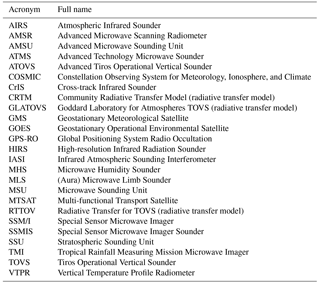
Table 1List of acronyms for reanalysis assimilated observations and radiative transfer models.
2.1 Reanalysis datasets
Fujiwara et al. (2017) provide detailed descriptions of the models, assimilation systems, and data inputs for the reanalyses used here in their overview paper on S-RIP. We compare the four most recent high-resolution full-input reanalyses for all winters with data available from the beginning of the “satellite era” in 1979. All of our analyses are done using daily 12:00 UT fields from each reanalysis dataset (we have tested the sensitivity of our analyses to using 00:00 UT data and have found we get virtually identical results). Because of the importance of resolution, especially in the vertical dimension, in representing the polar lower stratosphere and threshold processes in general (see, e.g., Manney et al., 2017), we start our analyses from reanalysis data on the native model levels and at or (in the case of spectral models) near the native horizontal resolution. Please see Table 1 for a list of relevant acronyms that we use below to describe the instruments, radiative transfer models, etc., that are used by the reanalyses.
2.1.1 CFSR/CFSv2
NCEP-CFSR/CFSv2 is a global reanalysis wherein CFSR covers 1979 through 2010 and CFSv2 covers 2011 through the present (Saha et al., 2010, 2014). The data are produced using a coupled ocean–atmosphere model and 3D-Var assimilation. CFSR/CFSv2 uses the CRTM for satellite radiance assimilation. The model resolution is T382L64, but the data used here are on a 0.5∘ × 0.5∘ horizontal grid on the model levels (available through 2015); vertical grid spacing in the lower stratosphere ranges from about 0.8 km near 100 hPa to 1.3 km near 10 hPa. CFSR did make an undocumented update to their assimilation scheme in 2010 (Long et al., 2017). Furthermore, in the transition from CFSR to CFSv2 in 2011, the resolution, forecast model, and assimilation scheme were all upgraded; CFSv2 is, however, intended as a continuation of CFSR and can be treated as such for most purposes (Saha et al., 2014; Fujiwara et al., 2017; Long et al., 2017); we thus treat these as a single reanalysis in this paper.
2.1.2 ERA-Interim
ERA-Interim (see Dee et al., 2011) is another global reanalysis that covers the period from 1979 to the present. The data are produced using 4D-Var assimilation with a T255L60 spectral model. ERA-I uses the version 7 RTTOV radiative transfer model for radiance assimilation. Here, we use ERA-Interim data on a 0.75∘ × 0.75∘ latitude–longitude grid (near the resolution of the model's Gaussian grid) on the 60 model levels. The spacing of the model levels in the lower stratosphere is about 1.2 to 1.4 km.
2.1.3 JRA-55
JRA-55 (Ebita et al., 2011; Kobayashi et al., 2015) is a global reanalysis that covers the period from 1958 to the present, and is produced using 4D-Var assimilation. The data from the JRA-55 T319L60 spectral model are provided on an approximately 0.56∘ Gaussian grid corresponding to that spectral resolution. JRA-55 uses RTTOV version 9.3 for satellite radiance assimilation. The JRA-55 fields on the model vertical levels have a vertical resolution of ∼1.2 to 1.4 km in the lower stratosphere.
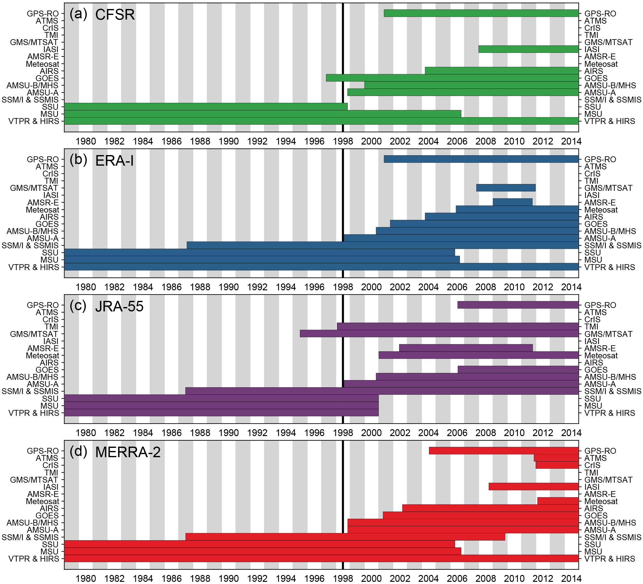
Figure 1Timeline for operational satellite instrument inputs to the reanalyses used herein: panels (a) through (d) show CFSR/CFSv2, ERA-I, JRA-55, and MERRA-2, respectively. Table 1 gives a list of the acronyms used here. Within the constraint of putting them in the same order for each reanalysis, the input datasets are stacked in approximately chronological order, with earliest on the bottom and latest on the top. The black vertical line is at the middle of 1998, near the time of the TOVS to ATOVS transition (see text). See Fujiwara et al. (2017) for a similar timeline but organized per instrument.
2.1.4 MERRA-2
MERRA-2 (Gelaro et al., 2017) is a global reanalysis produced by the National Aeronautics and Space Administration Global Modeling and Assimilation Office (NASA GMAO) covering 1980 to the present. It is based on the Goddard Earth Observing System (GEOS) 5.12.4 assimilation system, which uses 3D-Var assimilation with incremental analysis update (IAU) (Bloom et al., 1996) to constrain the analyses. MERRA-2 is intended to be a replacement for its predecessor, MERRA (Rienecker et al., 2011), as it includes many updates over MERRA (see, e.g., Bosilovich et al., 2015; Molod et al., 2015; Takacs et al., 2016). Changes between MERRA and MERRA-2 that may significantly affect representation of the lower stratosphere include the addition of new observation types in MERRA-2 (see Sect. 2.1.5, Fig. 1 and Fujiwara et al., 2017); an updated radiative transfer model for radiance assimilation; a different treatment of conventional temperature data; and assimilation of data that uses upgraded background error statistics, which control the magnitude and spatial extent of the impact of observations on the assimilated product.
The MERRA-2 data products are described by Bosilovich et al. (2016). All MERRA-2 data products used here are on 72 hybrid sigma-pressure levels that have about ∼1.2 km grid spacing in the lower stratosphere, and a 0.5∘ × 0.625∘ latitude–longitude grid. Data from MERRA-2 from its spin-up year, 1979, are not in the public MERRA-2 record, but we use data from late 1979 to start the analysis with the Northern Hemisphere (NH) 1979/1980 winter. We use the MERRA-2 “assimilated” (ASM) data collection (Global Modeling and Assimilation Office (GMAO), 2015) here, as recommended by GMAO, particularly for studies that require consistency between mass and wind fields (see, e.g., Global Modeling and Assimilation Office (GMAO), 2017; Fujiwara et al., 2017).
2.1.5 Timeline of satellite data inputs to DASs
Operational satellite observations are the primary data constraints on reanalyses at stratospheric levels. Additional constraints on temperature are provided by radiosonde and other conventional observations (Fujiwara et al., 2017). While conventional data are important in the lower stratosphere, especially at midlatitudes, their coverage is sparse in the NH polar region and very poor in the SH, so that these regions are mainly constrained by satellite radiance measurements.
Figure 1 shows these satellite inputs (see Table 1 for the definitions of the acronyms) for each of the reanalyses used here, shown as stacked timelines to facilitate comparison of changes in data inputs between reanalyses. Up through about 1994, all of the reanalyses relied primarily on the TOVS instruments (SSU, MSU, VTPR, and HIRS), and (except CFSR/CFSv2) SSM/I and SSMIS. Between 1995 and 2002, there are several changes in the data inputs, and the inputs begin to vary more among the reanalyses. In recent years, MERRA-2 has assimilated Meteosat, IASI, CrIS, ATMS, and GPS-RO observations. IASI, CrIS, and ATMS are not assimilated in any of the other reanalyses. A change with a large impact on stratospheric temperatures overall is the transition from TOVS (with MSU and SSU) to ATOVS (with AMSU-A and AMSU-B/MHS); Fig. 1 shows that this transition is handled/timed differently among the reanalyses: for instance, although all reanalyses introduce AMSU-A at just about the same time, JRA-55 stops assimilating the TOVS instruments' data by 2000, whereas the others continue until 2006 (except for an immediate cutoff of SSU by 1999 in CFSR/CFSv2). Long et al. (2017) showed that this transition had a profound impact on the differences in zonal mean temperatures among the reanalyses, with a shift toward much better agreement after the transition.
While there are significant differences in how the reanalyses handle changing input data and which new data sources they include, the majority of the data inputs are the same for all of these reanalyses. We must thus keep in mind the possibility that similar spurious features represented in multiple reanalyses could arise from using the same (imperfect) data sources.
2.2 Methods
The methods and diagnostics used herein are largely the same as those used by Lawrence et al. (2015). In the subsections to follow, we describe the reanalysis fields we use, and how we prepare them and derive the polar processing diagnostics from them. We also provide some information on additional analysis techniques that we use to help interpret our results.
2.2.1 Preparation of meteorological fields
The two meteorological fields necessary to derive most of the diagnostics used herein are temperatures and PV on isentropic surfaces. In the results we present later, we show temperature diagnostics on pressure surfaces, and vortex diagnostics on isentropic surfaces; as will be discussed, we also calculate and use some temperature diagnostics on isentropic levels.
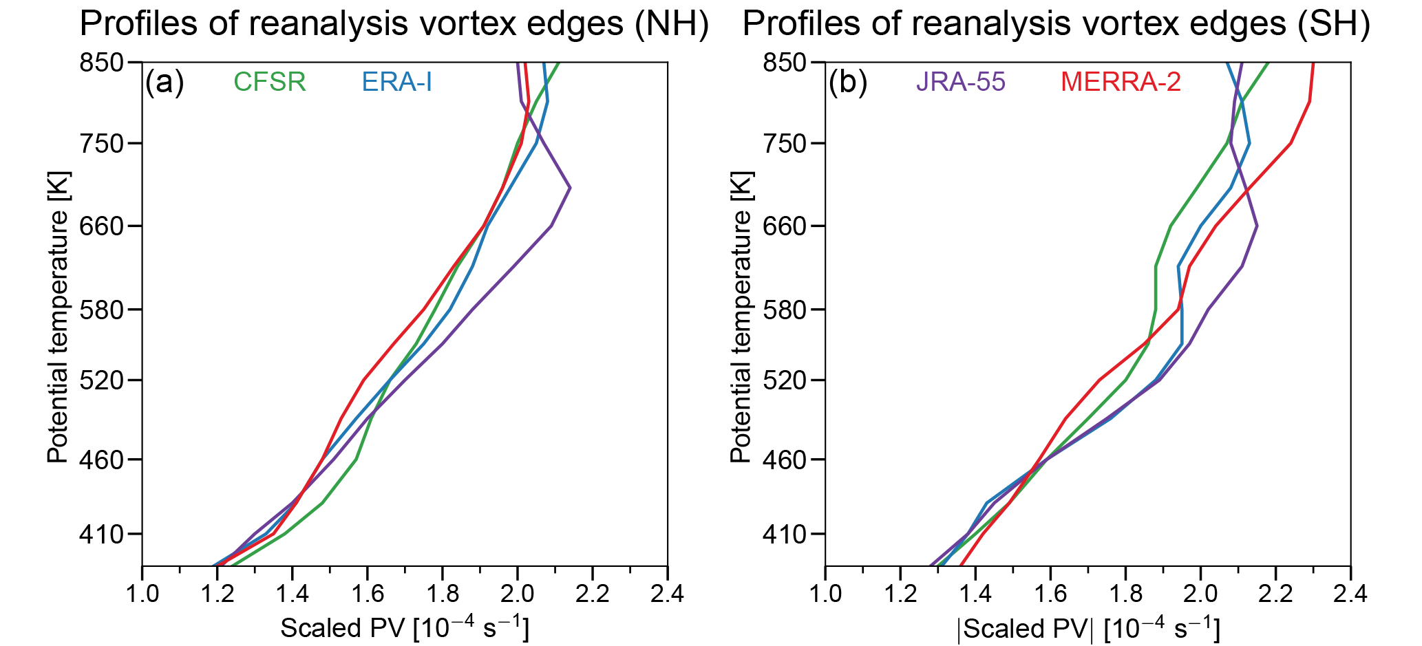
Figure 2Potential temperature profiles of the reanalysis vortex edges determined from climatological maximum PV gradients expressed as scaled PV for the NH (a) and the SH (b) . Green, blue, purple, and red indicate CFSR/CFSv2, ERA-I, JRA-55, and MERRA-2, respectively.
Of the four reanalyses described in Sect. 2.1, only MERRA-2 provides potential vorticity on its model levels. CFSR/CFSv2, ERA-Interim, and JRA-55 have isentropic PV available, but these products are only provided on a sparse set of isentropic levels, with very few common levels between the reanalyses. ERA-Interim provides absolute vorticity on model levels, and CFSR/CFSv2 provides relative vorticity; thus to get the vertically resolved PV fields that we need, we derive PV for these reanalyses using their provided vorticity, temperature, and pressure fields on the model levels. In the case of JRA-55, we use the zonal and meridional wind components to first calculate relative vorticity, which we then use in combination with temperature and pressure to calculate PV on the model levels. While a thorough evaluation of biases that may arise from using different types of PV calculations for different reanalyses would be valuable, it is beyond the scope of this paper. We think, however, that data users will most likely use the most direct calculation to get from the provided fields to the model level PV (as we have), and thus the fields we are comparing are those that are most likely to be used in practice. When calculating polar processing diagnostics, we scale the PV fields into vorticity units as in Dunkerton and Delisi (1986) by dividing the PV by a standard value of static stability calculated from assuming a vertical temperature gradient of 1 K km−1 and a pressure of 54 hPa on the 500 K isentropic level. We use this scaling so that the scaled PV (sPV) values are of the same order of magnitude at different levels throughout the stratosphere.
Since the reanalyses are all on different model levels, we use the reanalyses' temperature and pressure fields to vertically interpolate their temperature and PV fields to a common set of fixed pressure and isentropic surfaces. We use a standard set of pressure and isentropic levels that have been used for several NASA satellite instrument datasets (see, e.g., https://cdn.earthdata.nasa.gov/conduit/upload/4849/ESDS-RFC-009.pdf, last access: 12 September 2018) including the Aura Microwave Limb Sounder (Livesey et al., 2015); these are 12 levels per decade in pressure, and their climatologically corresponding isentropic surfaces. For polar processing diagnostics, we limit our focus to 14 levels with pressures between approximately 120 and 10 hPa; these pressure levels and their corresponding isentropic surfaces are shown in Appendix A (Table A2).
2.2.2 Temperature and vortex diagnostics
The depletion of ozone in the lower stratosphere follows from a complex chain of processes that are highly dependent on meteorological conditions (see, e.g., Solomon, 1999; WMO, 2014, for reviews). The activation of chlorine requires the presence of PSCs, which form when temperatures are sufficiently low, and grow when temperatures stay low for sufficiently long periods of time (Hanson and Mauersberger, 1988; Solomon, 1999; WMO, 2014, and references therein). The catalytic ozone destruction cycles involving both chlorine and bromine further require sunlight, which is usually provided later in winter and spring when sunlight returns to the high-latitude polar regions. These chemical processes also require isolation from lower-latitude air, which is provided by the stratospheric polar vortex; the edge of the polar vortex acts as a barrier preventing transport and mixing, and thus the vortex acts as a containment vessel for the polar air where these processes take place (e.g., Schoeberl and Hartmann, 1991; Schoeberl et al., 1992). We thus examine polar processing diagnostics that primarily focus on lower stratospheric temperatures and the state of the polar vortex to assess the meteorological conditions conducive to ozone depletion. Unless specified otherwise, we focus on the months from December to March (DJFM) for the NH, and May to October (MJJASO) for the SH; these time periods cover roughly the full period during which polar processing takes place for most polar winters (see Sect. 3.1).
The temperature diagnostics that we use include minimum temperatures (Tmin) poleward of ±40∘ latitude, and the areas of temperatures (poleward of ±30∘ latitude) below PSC formation thresholds (APSC, or area T≤TPSC, where the subscript “PSC” may be replaced by “NAT” or “ice” to denote the specific type of PSC). For APSC, we specifically use the formation temperatures for solid nitric acid trihydrate (NAT; Hanson and Mauersberger, 1988) and ice particles on pressure levels, which we define using climatological profiles of HNO3 and H2O mixing ratios (see Appendix A and Table A1 for values). As a rule of thumb, the NAT threshold between 120 and 10 hPa ranges from roughly 198 to 187 K, respectively, and the ice threshold tends to be between 6 and 8 K below the NAT threshold. We stress that these thresholds are approximations, but they are convenient as proxies for PSC formation and chlorine activation. While most of the results we show herein for the temperature diagnostics are on pressure levels, we also calculate them on isentropic surfaces; for the diagnostics involving PSC thresholds, we assign the PSC thresholds on pressure levels to the isentropic surfaces that are roughly co-located (e.g., 520 K corresponds to 46.1 hPa). This is an additional approximation, but it allows us to keep the intercomparisons simple without having to calculate daily varying PSC thresholds for pressures/temperatures on isentropic levels or pre-computing climatological PSC threshold values from the reanalyses' fields. (Please see Appendix A and Table A2 for the pressure surfaces used, their corresponding isentropic surfaces, and the PSC threshold temperatures.) To mitigate issues with these approximations and test sensitivity to the thresholds, we also compute APSC with ±1 K offsets to the PSC formation temperatures.
The vortex diagnostics that we use include maximum gradients in sPV as a function of equivalent latitude (maximum sPV gradients, or MPVGs), which assess the strength of the vortex edge (e.g., Manney et al., 1994, 2011; Lawrence et al., 2015), and the area of the vortex exposed to sunlight (sunlit vortex area, or SVA). To calculate MPVGs, we bin sPV as a function of equivalent latitude (EqL, the latitude that would enclose the same area between it and the pole as a given PV contour; Butchart and Remsberg, 1986), numerically differentiate, and catalog the maximum value between ±30 and ±80∘ EqL. We use ±30∘ as a lower limit because relatively large PV gradients can be found in the tropics, which can dominate early/late in the season when the vortex is forming/decaying; we use ±80∘ as an upper limit because the small areas represented by points poleward of ±80∘ can vary much more dramatically than the lower EqLs, sometimes producing large gradients (e.g., Nash et al., 1996) that are not indicative of the vortex edge.
To calculate SVA, we calculate the area of the vortex that extends equatorward of the daily polar night latitude at 12:00 UT. The area of the vortex is determined by defining constant contours of sPV as the vortex edge over all years; herein we determined these vortex edges individually for each reanalysis from climatological seasonal averages of their maximum PV gradients (as determined above) from the extended periods of November through April for the NH, and April through November for the SH. We use periods that are longer than the DJFM and MJJASO periods we use for the intercomparisons because they help to include the formation and breakdown of the vortex. While constant vortex edges are a simplification, the ones we use here are defined for each reanalysis individually, and thus they inherently fold in any systematic differences that the reanalysis sPV fields may have. Furthermore, more common definitions of the vortex edge that provide daily varying values can be prone to giving spurious oscillations from day to day that could contaminate intercomparisons (e.g., Manney et al., 2007; Lawrence and Manney, 2018). Figure 2 shows the NH and SH profiles of vortex edges used for each reanalysis; it shows that the values obtained for each reanalysis and hemisphere are generally consistent, and that the largest differences between reanalyses below 850 K are around s−1.
Figure 3Time series of reanalysis ensemble mean (REM) (a, c, e) Arctic and (b, d, f) Antarctic climatological (1979/1980 through 2016/2017 in the NH, and 1979 through 2016 in the SH) minimum high-latitude (poleward of 40∘ latitude) temperatures; panels (a) and (b) show contour plots (blue/purple shades represent low temperatures and reds high temperatures). The horizontal black lines mark the 30 hPa and 70 hPa pressure levels for which line plots are shown in panels (c) and (d) and in (e) and (f), respectively. The shading in the line plots shows the range of REM values on each date, and the black line shows the average values. Note that the time period shown is longer in the SH than in the NH. The same color range is used for each hemisphere, with values from 180 to 220 K shown (blues to reds; all values below/above 180/220 K are shown in the deepest blue/red).
2.2.3 Derived diagnostics
Here, we describe some additional diagnostics that we examine later in the paper that are derived from the raw diagnostics we calculate (primarily those described above).
The winter mean volume of lower stratospheric air with temperatures below TPSC (VPSC) is a widely used diagnostic of polar processing potential. It is often expressed as a fraction of the vortex volume (VPSC∕VVort) to provide a measure that is independent of the substantial interannual and interhemispheric variations in vortex size (e.g., Rex et al., 2004, 2006; Tilmes et al., 2006; Manney et al., 2011; Manney and Lawrence, 2016; WMO, 2014). (Again, we replace the subscript “PSC” with “NAT” or “ice” to denote specific PSC types.) Hence, VPSC∕VVort represents the approximate fraction of the vortex (for a specified altitude range) in which temperatures are low enough for the formation of PSCs. Here, we calculate VPSC and the volume of the vortex using APSC and the area of the vortex on isentropic levels between 390 and 550 K. APSC is calculated as described above in Sect. 2.2.2; the area of the vortex is calculated similarly to SVA but instead by finding the total area within the PV contours representing the vortex edge. To get volumes, we assume each isentropic level is nominally representative of the volume of air midway between each level; for example, the 410 K level comes after 390 K and before 430 K, so 410 K is assumed to be representative of the altitude “width” between 400 and 420 K. The altitude widths of these nominal levels are determined using the Knox (1998) approximation; for the levels from 390 to 550 K, the Knox approximation gives a mean altitude differential between levels of 1.13 km with a minimum of 0.98 km, and a maximum of 1.30 km. These altitude differentials are then multiplied by the area diagnostics on each isentropic level (which are converted to km2), and summed over the vertical range to get volumes. The volume fraction is then VPSC∕VVort. In the results we show later on, we specifically show winter mean VPSC∕VVort; these winter means are taken over DJFM for the NH and MJJASO for the SH.
The SH vortex breakup is of considerable concern because it results in the dispersal of ozone-depleted vortex air over midlatitudes (e.g., Ajtić et al., 2003, 2004; Manney et al., 2005c; Pazmino et al., 2005; WMO, 2007). While ozone depletion in the Arctic has not yet been large enough for this to be an ongoing concern, vortex evolution during the 2011 Arctic vortex breakup led to significant areas of ozone-depleted air over populated regions associated with increased surface UV (e.g., Manney et al., 2011; Bernhard et al., 2012). To examine the variability and representation in reanalyses of the vortex decay in the lower-to-middle stratosphere, we examine approximate vortex decay dates, which we derive using the vortex area diagnostic on isentropic levels from 460 to 850 K. Here, we calculate vortex area with s−1 sPV offsets to the vortex edges shown in Fig. 2. To accomplish this, we examine NH vortex area between 1 December and 1 June, and SH vortex area between 1 May and 1 March; we have defined the decay date as the last day before which the vortex area is above 1 % of a hemisphere continuously for 30 days. We choose 1 % of a hemisphere as the limit because this threshold is only climatologically met at all levels at the beginning and end of the seasons when the vortex is forming or breaking down, which guarantees that any time the vortex is that small, it is either significantly disturbed or in the process of decaying. The 30-day limit was chosen to help guarantee that the vortex was sufficiently coherent beforehand. Finally, we use vortex edges with the positive sPV offset mentioned above to help remove the influence of small vortex fragments that can be present at the end of the season, which in some cases can add up to areas larger than 1 % of a hemisphere and lead to marginal scenarios that can skew the decay dates. The results we show herein are not highly sensitive to changing the area threshold or using vortex area with/without the sPV offset; except in some marginal cases that we discuss later on, adjusting the area threshold between 1 and 4 % only modifies less than 10 % of the cases (i.e., different years and levels) in all the reanalyses by more than 20 days in the NH and more than 10 days in the SH.
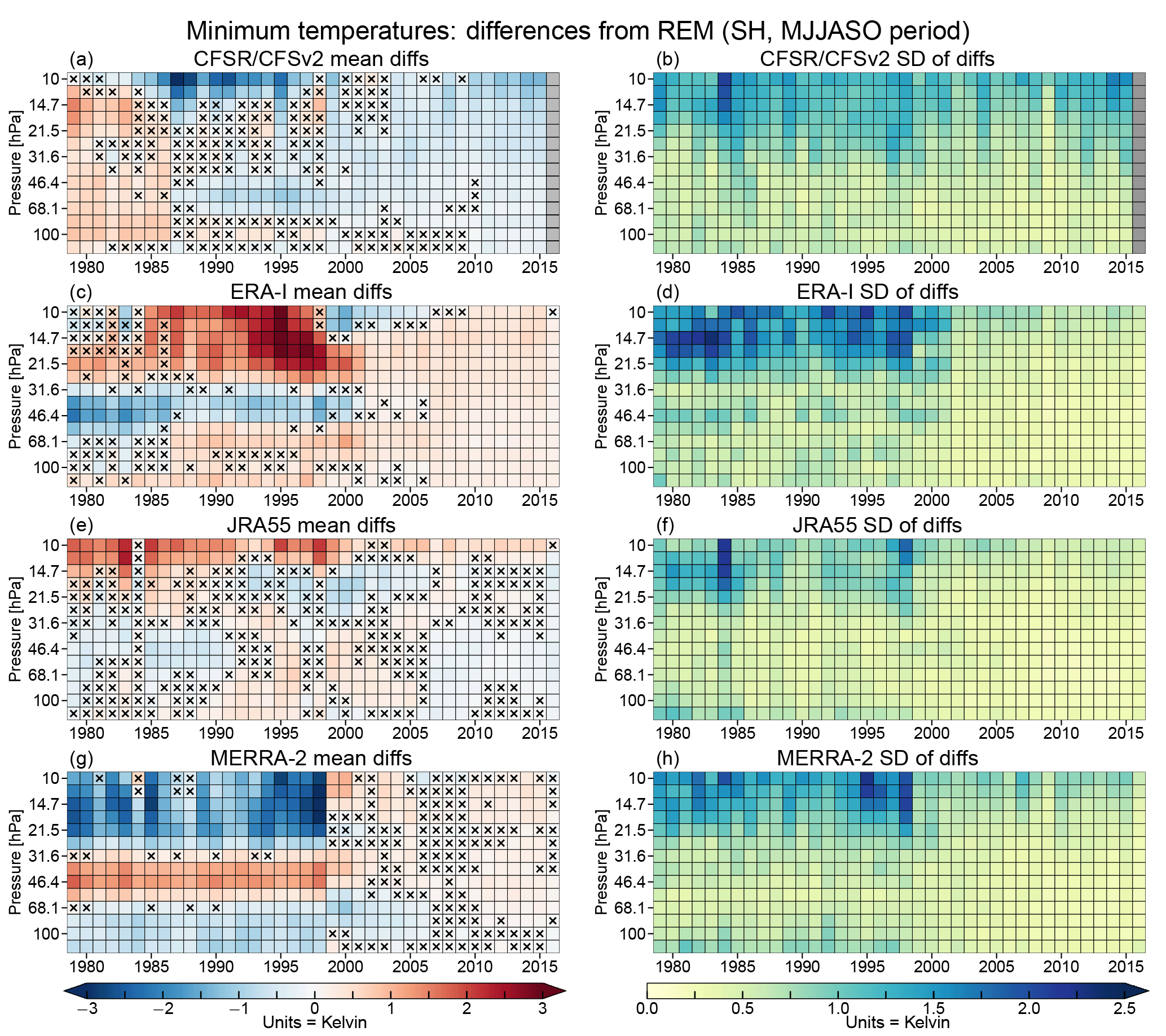
Figure 4SH winter season (MJJASO) (a, c, e, g) averages and (b, d, f, h) standard deviations of minimum temperature differences for each reanalysis from the reanalysis ensemble mean (REM) as a function of year and pressure for the 1979 through 2015 winters, concatenated from the individual years into pixel plots as described in the text. Columns of grey pixels indicate years with no data. Pixels with X symbols inside indicate years and levels where the differences from the REM are insignificant according to our bootstrapping analysis (see Sect. 2.2.4). Blues in the average difference panels show negative values (reanalysis less than the REM) and reds positive values (reanalysis greater than the REM); in the standard deviation panels, yellow/deep blue shades represent low/high standard deviations of the reanalysis differences, respectively.
2.2.4 Analysis techniques
For most of the results shown herein, we compare the diagnostics derived from each of the reanalyses to an average across all of the reanalyses, which is referred to as the reanalysis ensemble mean (REM). In Sect. 3.1 and 3.2, the comparisons primarily take the form of reanalysis differences from the REM (i.e., reanalysis minus REM).
Our analysis also includes a statistical significance test to determine whether the average differences between the reanalyses and the REM are statistically different from zero over a winter season. To accomplish this, we use a non-parametric bootstrap resampling technique that is useful for time series datasets called the stationary bootstrap (Politis and Romano, 1994). Bootstrapping methods for time series have generally relied on resampling blocks of consecutive observations to construct many artificial time series so that accuracy estimates can be made for sample statistics/estimators (e.g., Lahiri, 2003, and references therein). Rather than resampling random fixed-size blocks (which may or may not overlap) to construct artificial time series, the stationary bootstrap constructs artificial time series by resampling random blocks with random sizes determined from a geometric distribution with specified mean. Herein, we bootstrap the time series of differences from the reanalyses and the REM; we treat the difference time series for each reanalysis, diagnostic, and year individually while the vertical levels are resampled together. In nearly all cases (see the NH ANAT comparisons in Sect. 3.1 for the one exception), we perform stationary resampling with a specified geometric distribution mean of 10 (i.e., the expected block length is 10 days) and resample all the time series of differences 2×10⁵ times. We note that the results shown herein are not sensitive to the choice of the expected block length; we repeated our bootstrapping analysis for different expected block lengths between 5 and 15 days, and in all cases the results were nearly identical. Ultimately, we chose 10 days as a happy medium based on examinations of the decorrelation timescales of some of the difference time series. We then use the bootstrap percentile method to construct 99 % confidence intervals (CIs) of the average differences; the percentile method is known to have issues in cases with small sample sizes, but since we use a more strict 99 % CI and our time series are longer than 120 days, we expect that our estimates are robust (see discussion in DiCiccio and Efron, 1996, and references therein). When these 99 % CIs do not contain zero, we consider the average differences for the reanalysis minus the REM (for a specific level and year) to be indicative of persistent positive or negative differences. Thus, when statistical significance is mentioned hereinafter, we are referring to significance at the 99 % confidence level.

In the next two subsections, we show comparisons of temperature and vortex diagnostics as yearly time series of average differences and standard deviations calculated over the polar processing periods in each hemisphere (DJFM for the NH, MJJASO for the SH). We use these averages and standard deviations alongside the bootstrapping analysis to evaluate the agreement between the reanalyses.
3.1 Temperature diagnostics
Figure 3 shows the climatological values of minimum temperatures from the REM. The well-known difference in stratospheric temperatures between NH and SH (e.g., Andrews, 1989) is seen clearly, with the climatological period with temperatures below the NAT PSC threshold spanning approximately December through mid-February in the NH and mid-May through early October in the SH. The lowest temperatures are centered near 20 hPa at about the time of the solstice in the NH, and near 25 hPa approximately a month after the solstice in the SH. NH winter temperatures are lowest earlier in the season because of the prevalence of sudden stratospheric warmings (SSWs) in January and February in that hemisphere.
Figure 4 shows “pixel plots” of the winter mean differences in SH minimum temperatures from the REM (Fig. 4a, c, e, g), and the standard deviations of the differences (Fig. 4b, d, f, h) for each of the reanalyses. We use similar pixel plots herein for the other diagnostics and hemispheres discussed in Sect. 2.2.2. In these plots, each pixel represents a winter mean difference (i.e., reanalysis minus REM averaged over a winter period) or a standard deviation of the differences (i.e., the standard deviation of the reanalysis minus REM over the designated winter period) for a single year and vertical level.
The most striking feature shown in Fig. 4 is an overall improvement in the agreement around the turn of the century, particularly evident in MERRA-2 after 1998. This transition is also apparent in ERA-I, occurring between 1999 and 2001. In earlier years, ERA-I and MERRA-2 bracket the ensemble with differences up to ±3 K, which in later years drop to near 0.5 K. The SH CFSR/CFSv2 and JRA-55 minimum temperatures tend to reside between those of MERRA-2 and ERA-I and are generally close to the REM. In particular, the JRA-55 differences are marked as not statistically significant (at the 99 % confidence level, as described in Sect. 2.2) for many levels and years throughout the reanalysis period. The improvements after 1998 are largest at higher levels (where the differences and standard deviations are themselves largest), becoming less prominent, and less sudden, below about 50 hPa. MERRA-2 shows a change in sign of the differences in the upper levels (∼20–10 hPa). The overall convergence of the reanalyses after 1998–1999 is also seen as pronounced discontinuities in the standard deviations of the differences from the REM for ERA-I, JRA-55, and MERRA-2, with values frequently over 2 K before 1999 typically decreasing to below ∼0.8 K thereafter. The improvement is less evident in CFSR/CFSv2 with standard deviations greater than 1 K seen throughout the reanalysis period, particularly at pressures lower than ∼30 hPa. The 1998–1999 mark corresponds to the transition from assimilating TOVS to ATOVS radiances in all four reanalyses. In addition, in late 2002, MERRA-2 began assimilating the hyperspectral AIRS radiances, vastly increasing the number of data used in the Antarctic. ERA-I and CFSR/CFSv2 started ingesting AIRS data in 2004. Measurements of atmospheric thermal emissions in the 15 µm CO2 absorption continuum provided by this sensor are strongly sensitive to stratospheric temperature variations as demonstrated, for example, by Hoffmann and Alexander (2009). In addition, all the reanalyses considered here have assimilated data from GPS-RO instruments starting from 2001 in ERA-I and CFSR/CFSv2, from 2004 in MERRA-2, and from 2006 in JRA-55. The GPS-RO data also affect stratospheric temperatures indirectly by anchoring bias correction of radiance observations (Fujiwara et al., 2017).
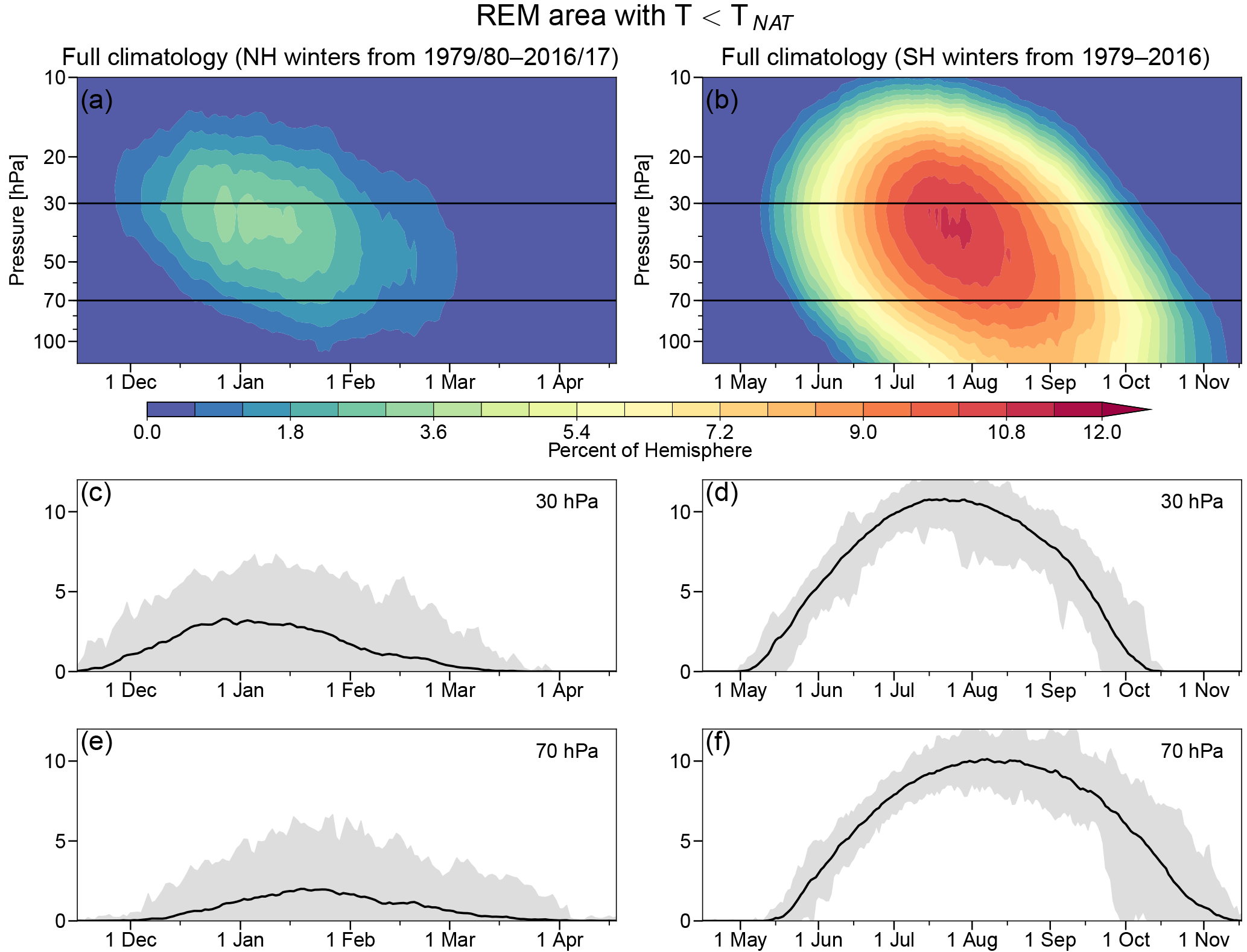
Figure 6As in Fig. 3 but for area with temperatures below the NAT PSC threshold. The color range in panels (a) and (b) goes from 0 % to 12 % of a hemisphere (blues to reds), with all values above 12 % shown in the deepest red.
During the years including roughly 1993 through 1998, larger differences and standard deviations are seen above about 30 hPa in ERA-I and MERRA-2. These differences are positive in the former and negative in the latter reanalysis, leading to a partial cancellation in the REM. Between 1986 and 2001, ERA-I exhibited a layered structure of differences from the REM: positive at pressures greater than ∼50 hPa and less than ∼30 hPa and negative in between. A similar structure but with the signs reversed is seen in MERRA-2 where it extends back to 1980 and ends sharply in 1998. Investigations in progress (Long et al., 2018) show that both MERRA-2 and ERA-I temperatures in the SH polar stratosphere have oscillations of up to about 3 K that are in opposite directions, leading to the structure of the differences seen here. (Note that the absence of oscillations in the other reanalyses does not imply better agreement with sondes; Long et al., 2018). After 2000, both reanalyses show slightly positive (and, in the case of MERRA-2, largely statistically insignificant) differences from the REM at most pressure levels. CFSR/CFSv2 shows mostly positive differences between 1979 and 1986; afterward, the differences are primarily slightly negative at most of the pressure levels shown.
While the main sources of stratospheric information for all the reanalyses before 1998 are the SSU and MSU instruments, different reanalyses use different radiative transfer models to assimilate them and apply bias correction differently (Wright et al., 2018). It is particularly difficult to speculate about changes in CFSR/CFSv2, since it has multiple discontinuities and biases related to stitching together execution streams and applying a bias correction in a model with a warm bias (Long et al., 2017). Thus, while we cannot pin down particular changes that are associated with the differences among the reanalyses prior to the introduction of ATOVS data, there are numerous factors that could contribute to this behavior.
Average differences in minimum temperatures in the NH (Fig. 5) show more complicated patterns of changes over the years than those seen in the SH. The differences are much smaller throughout the 38-year period, with maximum absolute differences near 1.5 K at the highest levels shown (mainly in the period from about 1994 to 2004), and more frequent years/levels where the average differences are not statistically significant. From roughly 10 to 25 hPa, the standard deviations do decrease from above ∼1 K to less than ∼0.75 K after around 1999, though (as was the case in the SH) they remain larger in CFSR/CFSv2 than in the other reanalyses. While there are indications of changes around 1999, particularly in ERA-I and MERRA-2 they are less abrupt and of smaller magnitudes than those in the SH, and it is not as clear that there is a uniform trend towards better agreement. As in the SH, the CFSR/CFSv2 differences are primarily positive before 1987 and negative afterwards. ERA-I shows mostly positive differences except near 10 hPa. The opposite is true for JRA-55, except for the period between 1998 and 2006 when the differences are near zero, but slightly positive (and many of them not statistically significant), at pressures greater than about 30 hPa. Similar to the SH case, MERRA-2 exhibits a layered structure of differences prior to 1998: positive between roughly 60 and 30 hPa, and negative outside of this layer. After 1998, the MERRA-2 differences are mainly positive, except at pressures greater than about 50 hPa, where the differences gradually change from negative to positive between 2005 and 2010, except at the lowest levels.
Figure 6 shows the REM climatological values of the area with temperatures below the NAT PSC threshold (ANAT) for the NH and SH winter seasons. As expected, these echo the patterns of minimum temperatures seen in Fig. 3, with the largest areas in the NH in early January, and in the SH in middle to late July. The great variability in the NH (see the grey envelopes in the line plots) results in the largest values being well above the climatological average, about 7 %–8 % of a hemisphere, but still much lower than the largest average values in the SH of over 10 % of a hemisphere.
Note that comparing differences in NH ANAT among the reanalyses is more difficult than doing so for the SH or for the other NH diagnostics. Because there is significant interannual variability in the onset, termination, and magnitudes of low temperatures in the NH (see both Figs. 3 and 6), there are many NH winters with relatively few days having temperatures below TNAT and thus many days with NH ANAT being zero. Thus, comparing differences among the reanalyses for the full DJFM time period can often be unfairly biased by the high occurrence of zeros, which artificially decreases the average differences and standard deviations. To allay this issue such that we fairly compare NH ANAT, we modify our analysis procedure as follows: we use time series of the REM NH ANAT in November through April on 30, 50, and 70 hPa to define approximate start and end dates for the periods having non-zero ANAT. We use 30 hPa to define the onset dates (because ANAT usually first becomes non-zero around this level; e.g., Fig. 6a), and 50 or 70 hPa to define the termination dates. More specifically, we define the onset dates for each year as the first day at 30 hPa having non-zero ANAT, and the termination dates as the latest day chosen by either 50 or 70 hPa having non-zero ANAT; both 50 and 70 hPa are used because termination most often happens latest around 70 hPa as seen in Fig. 6a, but in some winters it happens later around 50 hPa. This process gives us individual “NAT seasons” between 1979/1980 and 2016/2017; these have a median length of 85 days, with the minimum and maximum number of days being 40 and 126, respectively. We then use these truncated time series to define the average differences and standard deviations thereof. This modifies the bootstrapping procedure described in Sect. 2.2.4; we still perform 2×10⁵ stationary bootstraps for each year, but because the lengths of the time series vary, we also vary the expected block size for each year by specifying them as the nearest integer to the cube root of the time series lengths plus a constant offset of +5 (which ranges from 8 to 10 days for time series lengths between 40 and 126 days). As was found for the regular bootstrapping procedure, using different expected block lengths with offsets between 0 (3 to 5 days) and 10 (13 to 15 days) had very little effect on the statistical significance results.
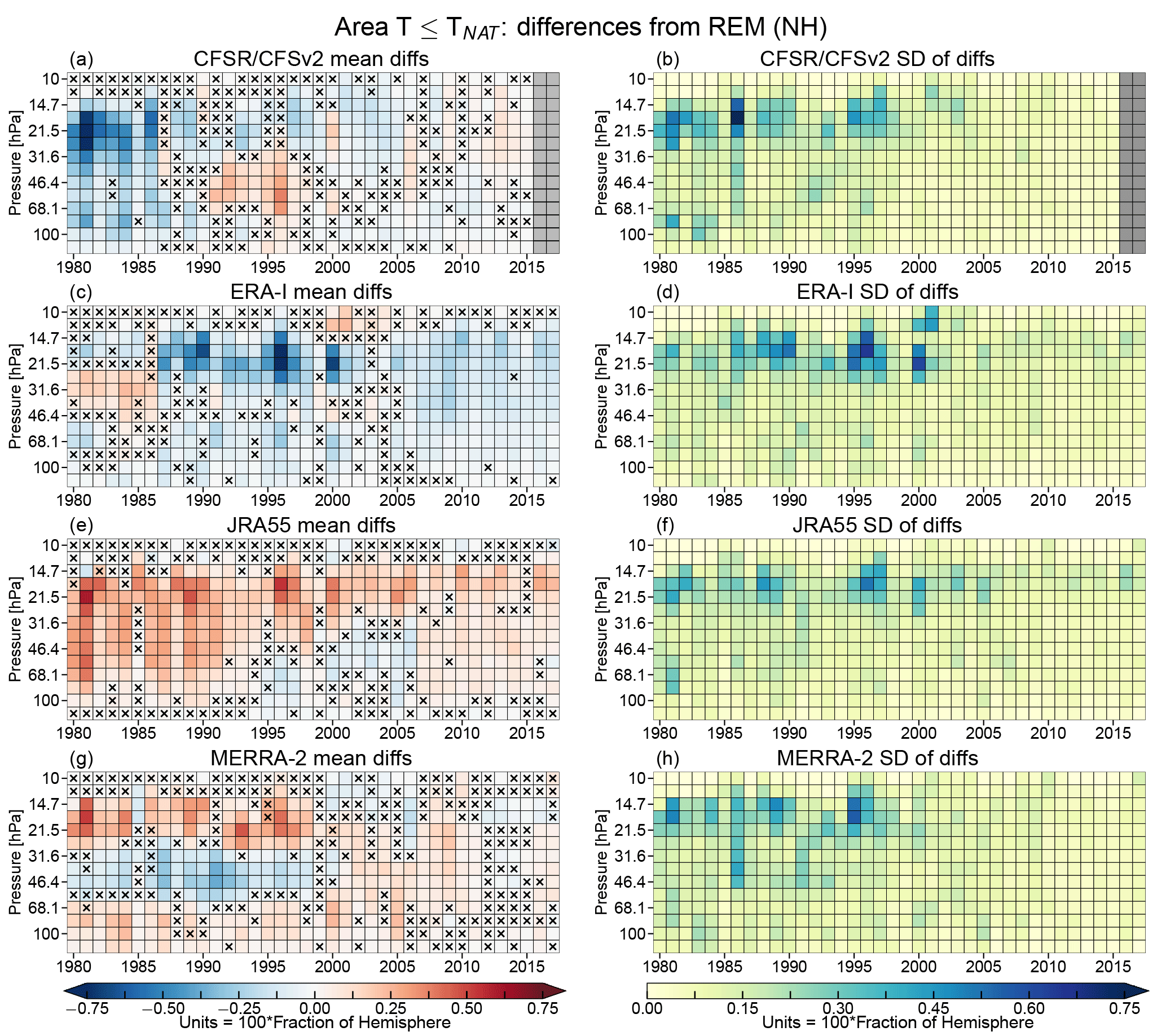
Figure 8As in Fig. 7 but for the NH. See text for explanation of date ranges used for the calculations.
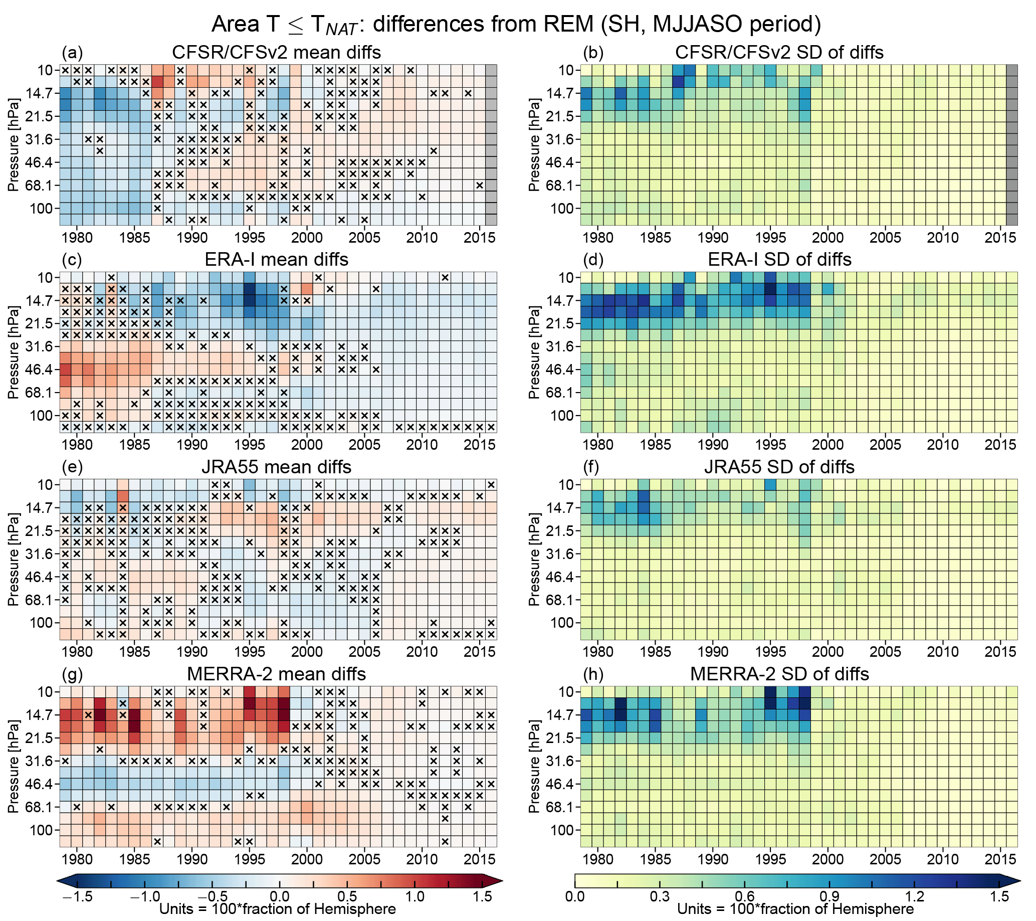
Figure 7 shows ANAT differences from the REM for the SH winter seasons. There is a very apparent sudden decrease in the seasonal standard deviations of the differences at levels above ∼25 hPa after 1998 similar to but much more pronounced than in the case of minimum temperatures. The 1998–1999 boundary is less obvious in the average differences for CFSR/CFSv2 and JRA-55 but is apparent in ERA-I and MERRA-2. By these metrics, all four reanalyses converge toward better agreement following the TOVS/ATOVS transition. The patterns of differences largely mirror (in an opposite sense) the patterns shown in Fig. 4; that is, there tend to be positive/negative differences from the REM in ANAT wherever there are negative/positive differences from the REM in minimum temperatures. ERA-I and MERRA-2 display layered difference structures prior to 1998; these layers of positive and negative differences are separated by approximately the 30 and 70 hPa pressure levels. As in the case of the minimum temperatures, the layered structures are more persistent in MERRA-2, extending between 1980 and 1998, whereas the one in ERA-I becomes apparent after 1986. JRA-55 and CFSR/CFSv2 are more often closer to the REM in terms of both the mean differences and the standard deviations. For CFSR/CFSv2, at pressures greater than 20 hPa, the differences are mostly negative (smaller ANAT) prior to 1986, and mostly positive thereafter. No clear pattern is apparent for JRA-55, although after approximately 2005 each reanalysis generally has a uniform sign of the differences from the REM in the deep layer between 120 and 10 hPa. Overall, the largest mean differences tend to be at levels above (pressures lower than) ∼20 hPa prior to 1998, with mean differences as large as ±1.5 % of a hemisphere; at higher pressures in the lower stratosphere where the bulk of polar processing takes place, average differences are often well within ±1 % of a hemisphere during this time and within ±0.5 % of a hemisphere thereafter. Despite the better agreement, in later years, many of the differences remain statistically significant after 1998; given the low standard deviations, these results indicate small but persistent (i.e., roughly constant) differences relative to the REM.
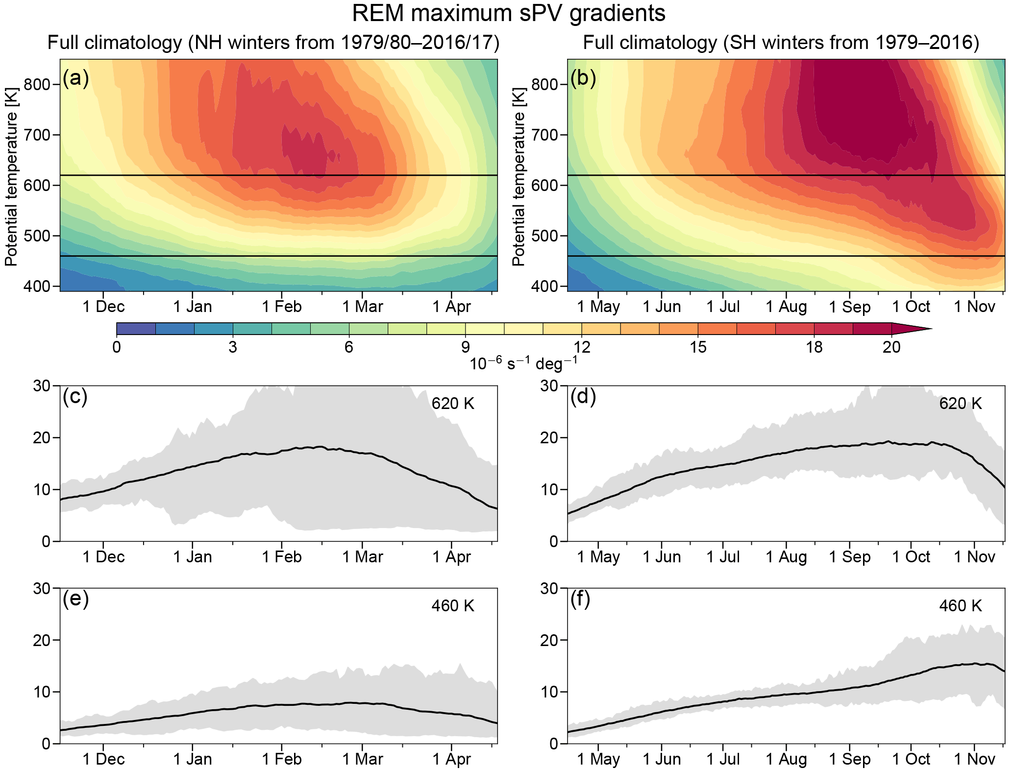
Figure 9As in Fig. 3 but for maximum sPV gradients. The color range in panels (a) and (b) is from 0 to 20 scaled PV gradient units (PVGUs) (blues to reds), with all values over 20 shown in the deepest red.
Differences in NH ANAT from the REM (Fig. 8) show more complex patterns than those in the SH and less of an obvious convergence toward better agreement after 1998, similar to the corresponding Tmin differences. The differences do decrease after about 2000, with most average differences being between ±0.25 % of a hemisphere. JRA-55 does show a narrow band of slightly larger positive differences continuing into the later years between about 30 and 15 hPa. MERRA-2 and ERA-I exhibit a pattern of opposing differences in this same layer between 1986 and 1998, but a layered structure of positive and negative differences at the lower levels is mostly only apparent in MERRA-2, consistent with the structure of the Tmin differences seen in Fig. 5. Overall, the differences are mostly negative in CFSR/CFSv2 and ERA-I, and positive in JRA-55 and MERRA-2, but there is a considerable dependence on time and pressure for all the reanalyses. As was the case for the SH, the standard deviations decrease over time with the largest values seen before 2001. There is a considerable year-to-year variability in the standard deviations at the higher levels in the earlier period with some years especially standing out (1986 in CFSR/CFSv2 and MERRA-2, 1996 in ERA-I and MERRA-2, and 2000 in ERA-I). These highest levels tend to be where ANAT is climatologically marginal (see Fig. 6).
Overall, the patterns of differences in ANAT qualitatively follow those in Tmin in both hemispheres: positive/negative differences in ANAT correspond to negative/positive differences in the minimum temperatures, as expected. However, the patterns of statistical significance are often different. For example, broad patches of largely statistically insignificant differences in Tmin in MERRA-2 and JRA-55 in both hemispheres after 1998 do not always translate into differences in ANAT marked as not significant. Furthermore, the largest (most positive) values of one diagnostic do not always yield the smallest (most negative) ones in the other, and vice versa. Even more strikingly, the patterns of standard deviations, while overall similar, do not exhibit a simple monotonic relationship with those in Tmin and generally display much more year-to-year variability before 2000. This is not unexpected as ANAT differences depend not only on overall temperature biases but also on the morphology of the fields (e.g., spatial patterns or gradients), which varies from year to year and, to a certain extent, among the reanalyses. While closely related, the ANAT and Tmin statistics represent different diagnostics and elucidate different aspects of the reanalyses' differences in relation to polar processing.
3.2 Vortex diagnostics
Figure 9 shows the NH and SH climatologies of REM MPVGs. The evolution of MPVGs is quite similar in both hemispheres, particularly above 500 K; the gradients in sPV gradually increase over time, reaching maxima in roughly mid-February in the NH and early October in the SH. These patterns largely reflect two effects: one is the seasonal cycle of the vortex building up strength and subsiding. The other is the build-up effect from wave breaking and mixing/erosion of PV in the surf zone (the region of low-magnitude PV outside the vortex, e.g., McIntyre and Palmer, 1984) over the season, which can act to sharpen the gradients of PV in the vortex edge region. Generally, MPVGs provide a measure of the strength of the vortex edge as a transport barrier. For simplicity, in the discussion of results below, we will refer to s−1 deg−1 as 1 scaled PV gradient unit, or 1 PVGU.
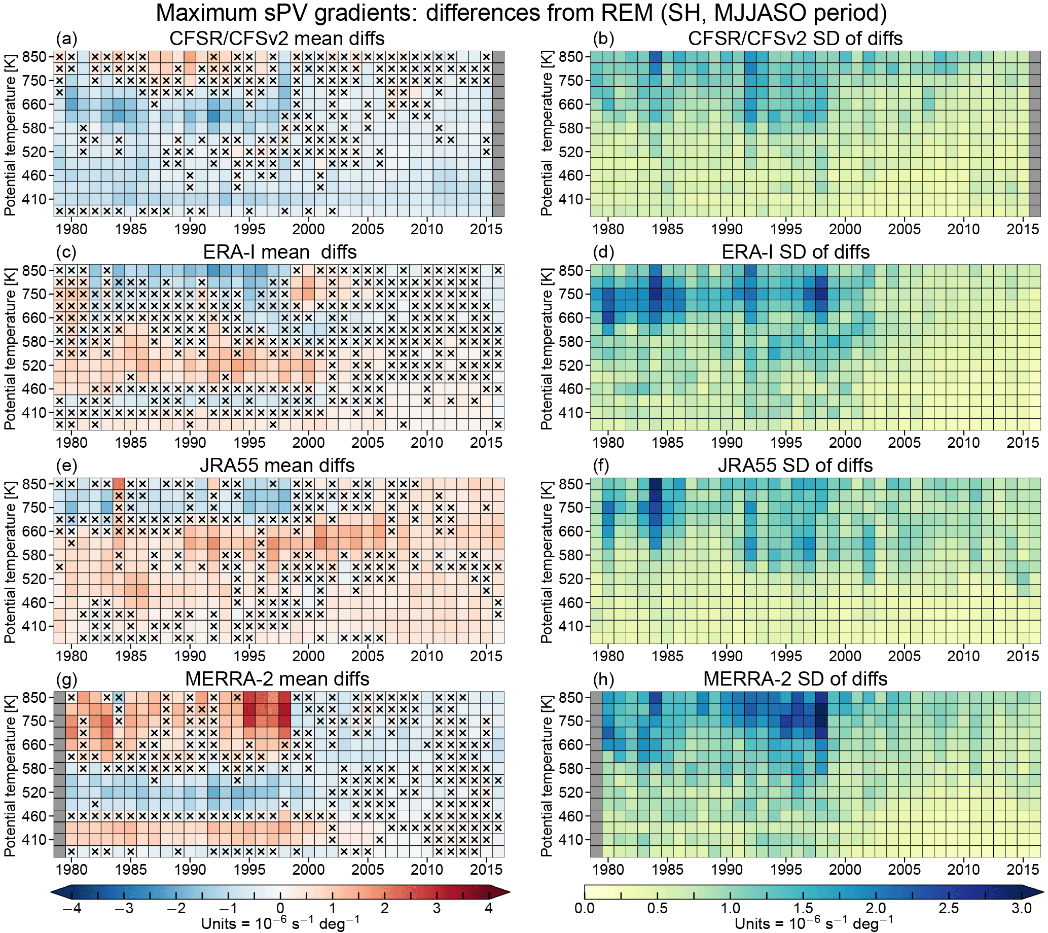
The averages and standard deviations of differences from the REM SH MPVGs are shown in Fig. 10. Through about 1998–2000, ERA-I and JRA-55 show similar patterns of differences from the REM, with a band of near-zero (for JRA-55) or small negative (for ERA-I, magnitudes up to ∼1.5 PVGUs) differences that are usually not statistically significant (at the 99 % confidence level, as described in Sect. 2.2) below about 460 K, positive differences between about 460 and 660 K, and negative differences above. The ERA-I differences are generally not statistically significant between 580 and 750 K. In the same time period, MERRA-2 shows an approximately opposite pattern, with negative differences from about 460 to 660 K and positive differences above and below; from about 1995 to 1999, MERRA-2 shows large average differences up to about 3.5 PVGUs above 700 K. In contrast to the banded structures in the other reanalyses, CFSR/CFSv2 generally shows small-magnitude negative differences across the levels and period, except during the period including 1985 through 1996 above about 700 K. The seasonal standard deviations of the differences are relatively small (usually on the order of 0.5–1.5 PVGUs), suggesting that statistically significant differences in the reanalyses typically represent differences that are more systematic in nature for MPVGs at these levels and times. The standard deviations tend to increase with height, especially at levels in the middle stratosphere above about 660 K where the differences can exceed 2.5–3 PVGUs. CFSR/CFSv2 and JRA-55 generally show slightly lower standard deviations than ERA-I and MERRA-2, and MERRA-2 shows a cluster of years between about 1994 and 1998 with large standard deviations above 700 K. After about 1998, there is a noticeable shift toward better agreement in most regions, similar to that seen in the SH temperature diagnostics. CFSR/CFSv2 and JRA-55 do not show an obvious improvement below about 550 K but already had close agreement with the REM there. In ERA-I and MERRA-2, most regions show small (magnitude less than 1 PVGU) differences that are not statistically significant after 1998. This shift toward better agreement is also reflected in the standard deviations, which markedly decrease in all the reanalyses, especially at levels above about 580 K. Similar to the temperature diagnostics, the TOVS to ATOVS transition most likely played a large role in this shift, with differences in the handling of this transition and the addition of AIRS radiances in 2002 also expected to be significant factors.
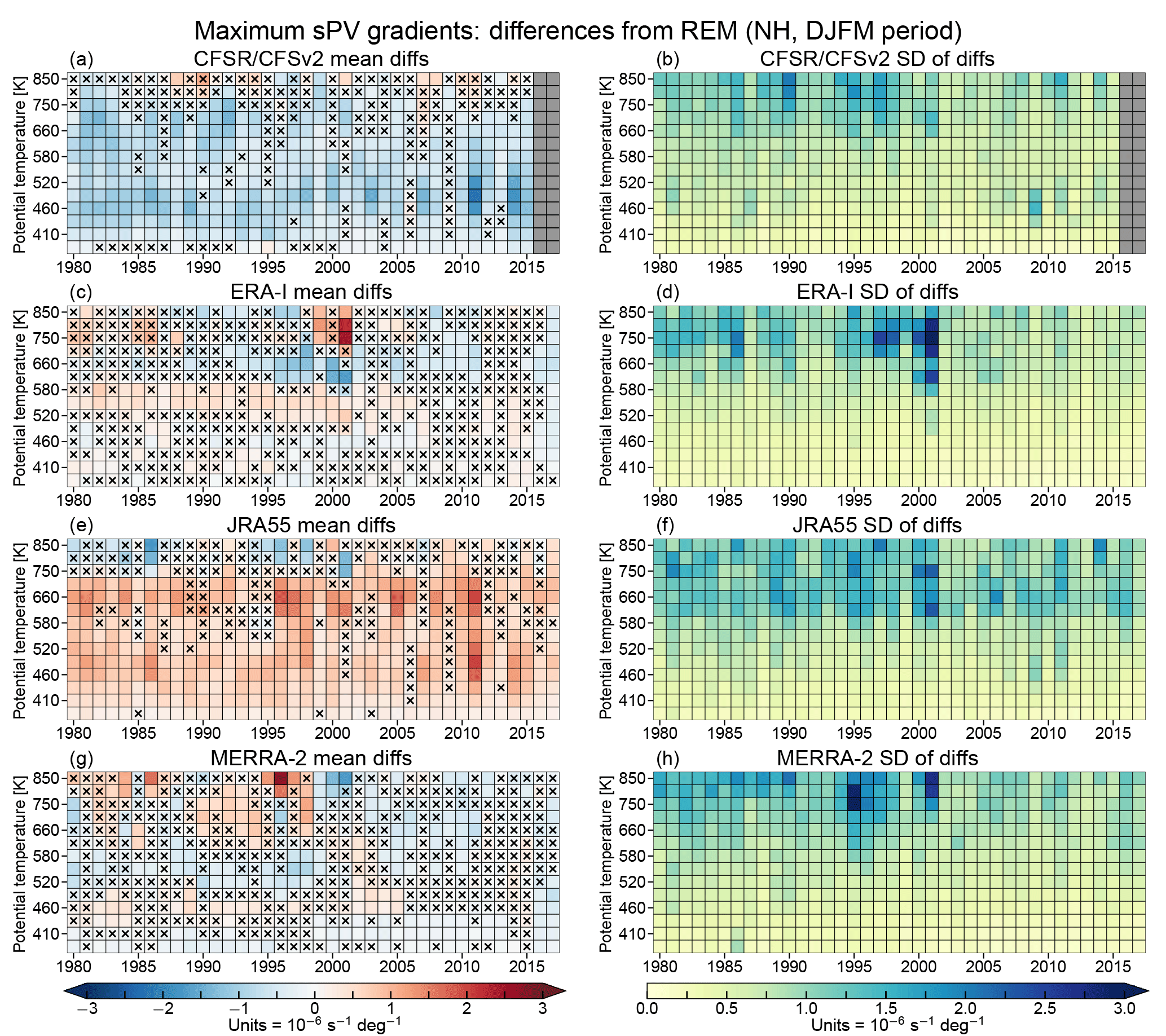
Differences in NH MPVGs from the REM (Fig. 11) indicate that CFSR/CFSv2 generally has smaller, and JRA-55 larger, PV gradients than the REM at levels up through about 750 K. ERA-I and MERRA-2 show smaller and less systematic patterns of differences that typically are not statistically significant. ERA-I does show a small vertical region with significant positive differences from the REM between 520 and 580 K until about 2001, similar to its pattern for the SH but with overall smaller differences. The standard deviations of the differences are largely consistent among the reanalyses; other than a few standout cases in ERA-I and MERRA-2 (1994/1995 in MERRA-2 and 2000/2001 in both), the standard deviations tend to increase consistently with height from less than 0.8 PVGUs at the lowest levels, to about 1.5+ PVGUs at the highest levels. There is some indication of convergence toward better agreement in MPVGs after roughly 2001 in MERRA-2 and ERA-I (when the reanalyses, except JRA-55, began assimilating AIRS radiances; Fig. 1), though most differences from the REM for these two reanalyses were not statistically significant even in the earlier years. No qualitative improvement in agreement with the REM is apparent in the CFSR/CFSv2 or JRA-55 differences, but the standard deviations of the differences do seem to decrease slightly above about 580 K for years after 2001.
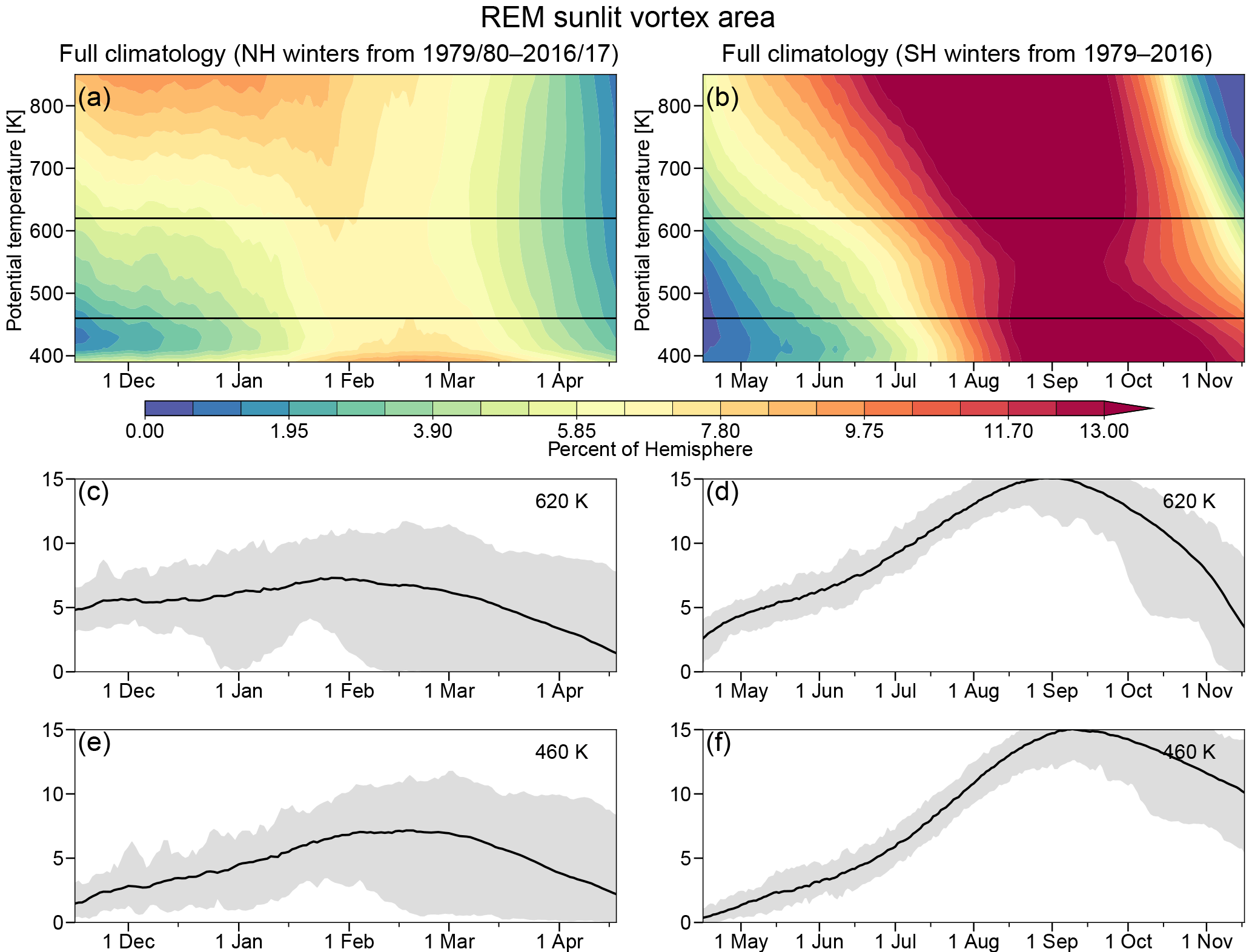
Figure 12As in Fig. 9 but for sunlit vortex area. The color range in panels (a) and (b) is from 0 % to 13 % of a hemisphere (blues to reds), with all values over 13 % shown in the deepest red.
Figure 12 shows the REM climatologies of SVA for both hemispheres. As was the case for MPVGs, the seasonal patterns of SVA for both hemispheres are similar. In this case, the patterns are largely due to the lack of sunlight early in the winter season, which gradually returns later on. However, there are notable differences between the hemispheres, particularly that SVA tends to be smaller in the NH; this is because the NH polar vortex is almost always smaller than its SH counterpart. The NH also shows relatively larger values in early winter above about 650 K, resulting from the NH vortex being more often disturbed and shifted to lower latitudes within sunlight. During individual winters, and given sufficiently low temperatures, the amount of vortex air exposed to sunlight at any time is generally indicative of the amount of air where ozone depletion can take place.
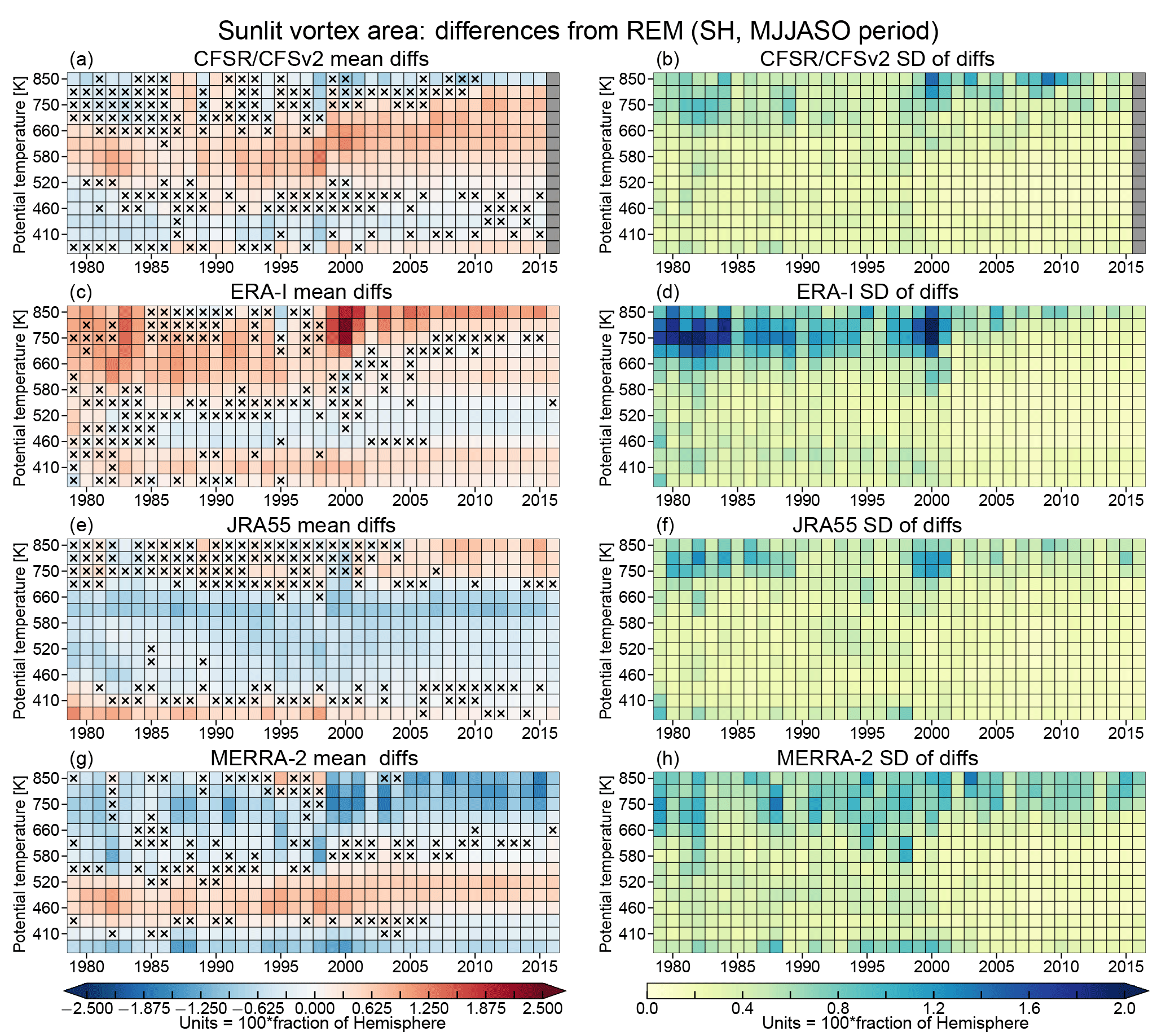
The averages and standard deviations of differences of SH SVA from the REM are shown in Fig. 13. There are some persistent patterns of differences among the reanalyses; JRA-55 SVA is consistently smaller than that from the REM between about 430 and 700 K and larger above and below. Above about 700 K, JRA-55 differences are generally not statistically significant through about 2003, after which each of the other reanalyses evaluated had started assimilating AIRS radiances (see Fig. 1 and Fujiwara et al., 2017). The other reanalyses generally show sandwiched structures of negative and positive differences: MERRA-2 (ERA-I) shows positive (negative) values between 430 and 520 K, with negative (positive) values above and below. CFSR/CFSv2 shows positive values between about 490 and 660 K, and small (often not statistically significant) negative values at higher and lower levels; in this case, the band of positive differences extends to higher levels after 1998. In the top several levels (approximately 750 to 850 K), agreement of the reanalyses with the REM appears to degrade starting about 1999–2000: ERA-I and MERRA-2 show a decrease in the number of values that are not significantly different from zero, while JRA-55 shows a similar decrease starting around 2003–2004. MERRA-2 differences increase in magnitude in this region and time period, and those in JRA-55 change from negative to positive, while ERA-I shows increased differences, near/over 2.5 %, at the highest levels in 1999–2001. CFSR/CFSv2 shows an increase in the significance of the differences at these levels after 2010 (the time of the CFSR to CFSv2 transition). The standard deviations of the differences are the highest at levels above 660 K where they are often above 1 % of a hemisphere. These are more pronounced in ERA-I, which shows standard deviations often ranging above 1 %, with some years reaching over 2 % above 660 K. Some slightly larger (0.4 % to 0.8 %) standard deviations are also seen at the lowest levels (390 and 410 K), which are around the top of the subvortex region for the SH. After 2001, the standard deviations of differences are generally less than 0.4 % of a hemisphere at most of the levels between 390 and 750 K in all the reanalyses, suggesting a small shift towards more consistent SVA differences compared to the REM among the reanalyses. Examination of the reanalyses' differences in vortex area from those in the REM reveal they are nearly identical to those for SVA, indicating that the differences are largely dominated by differences in the area enclosed within the vortex edge contours.
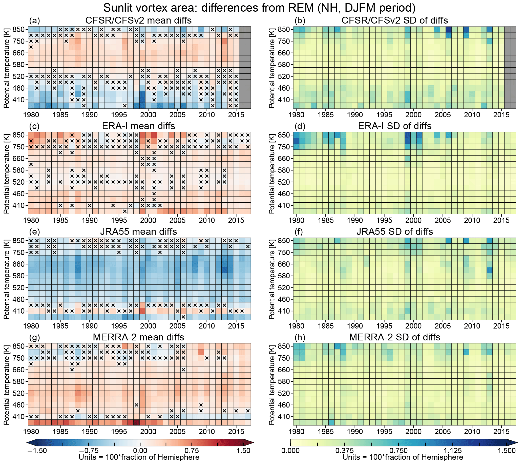
The patterns of averages and standard deviations of differences in SVA for the NH (Fig. 14) are quite different from those in the SH: MERRA-2 and ERA-I show overall positive differences (except for narrow bands of small differences at the highest levels that are not significant), while JRA-55 shows overall negative values. CFSR/CFSv2 shows negative values below about 520 K and at 800 and 850 K, with positive values in between. There is no obvious indication of a decrease in the magnitude of the differences over the period compared. The standard deviations of NH SVA differences from the REM generally look consistent between the reanalyses, with the largest values greater than 0.7–1.2 % of a hemisphere usually confined to a band of levels between 700 and 850 K. At lower levels, however, the standard deviations are quite small throughout the period, generally on the order of 0.5 % of a hemisphere or less; CFSR/CFSv2 shows slightly higher values below about 460 K. As was the case for the SH, the SVA differences are dominated by differences in total vortex area among the reanalyses. Thus, while there is no consistent change in agreement over the years, our results indicate persistent differences in the size of the contours used to define the vortex edges and hence some persistent differences in the isentropic PV fields (reflected in differences in the PV values at which the maximum PV gradients are located).
3.3 Derived vortex–temperature diagnostics
The diagnostics shown in the following subsection are derived from the temperature and/or vortex diagnostics shown in the previous two subsections.
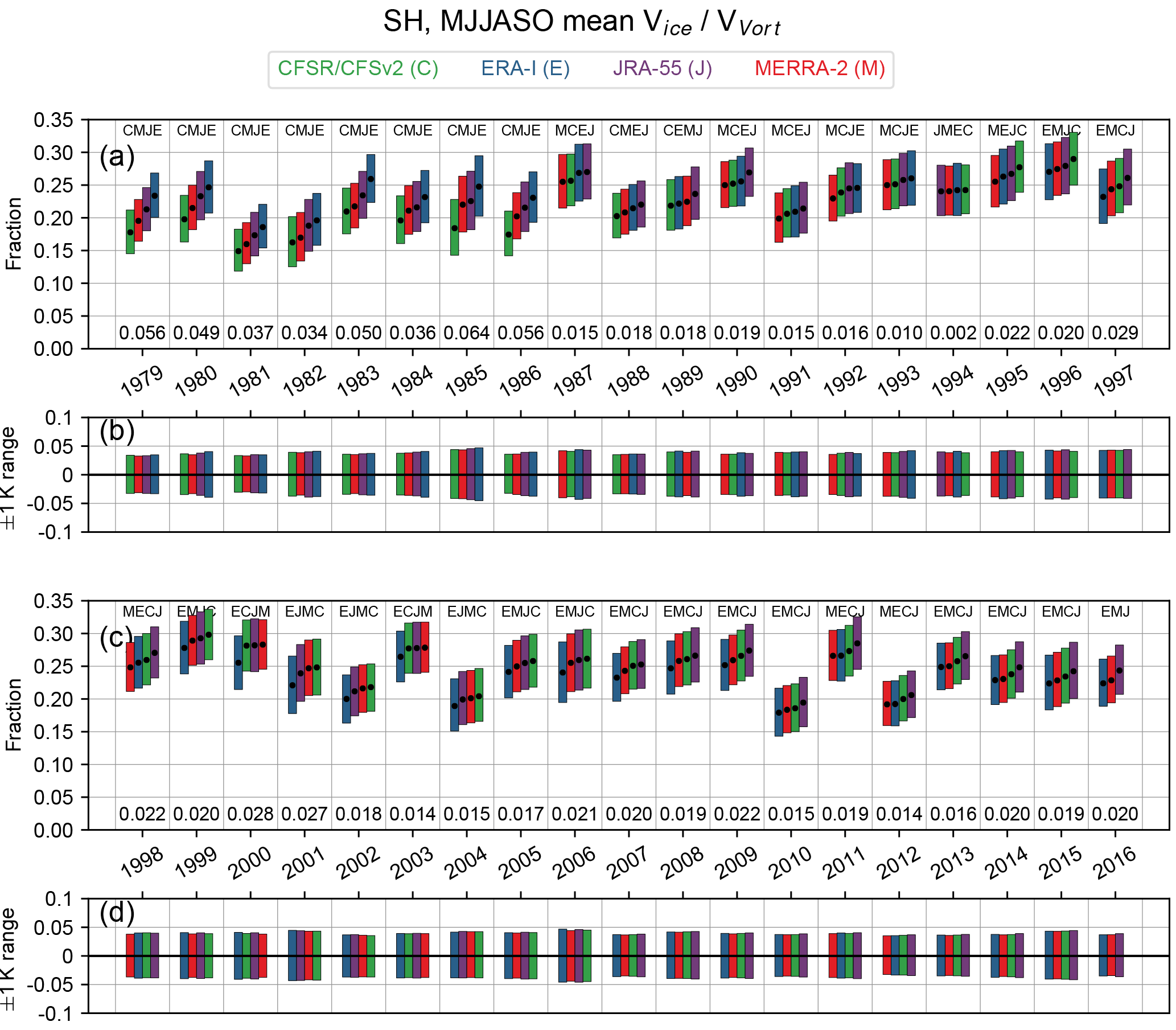
Figure 15Winter means of the fraction of vortex volume between the 390 and 580 K isentropic surfaces with temperatures below Tice in the SH (a, c), and range of values obtained for the ±1 K sensitivity tests (b, d). The colored bars show the range of values obtained from the tests of sensitivity to the PSC threshold temperature used (see Sect. 2.2.2), while the black dots show the value for the “central” threshold temperature. The winter mean is calculated over the full MJJASO period. For each year, the reanalyses are ordered from smallest central value on the left to largest central value on the right; this order is also given as a text string at the top of the column for each year. The numbers at the bottom of each year's column indicate the difference in winter mean fraction between the largest and smallest central values for the winter season (i.e., between the rightmost and leftmost black dots). In the range panels (b, d), the range about the central value (black dots in a and c) is shown for each reanalysis. Green, blue, purple, and red indicate CFSR/CFSv2, ERA-I, JRA-55, and MERRA-2, respectively.
Figure 15 shows the winter mean volume of temperatures below Tice in the SH expressed as a fraction of the vortex volume, calculated for the central PSC threshold and the ±1 K sensitivity thresholds (see Sect. 2.2.2). Keeping in mind that Tice was estimated assuming nominal pressure levels for isentropic levels (see Sect. 2.2.2), which can result in significant overestimates of areas/volumes, Fig. 15 shows that the volume fraction of cold air is relatively constant from year to year. Generally, the fractions of the vortex are between 0.20 and 0.30 each year, with sensitivities to the ice threshold offsets often less than ±0.05. During the winters of 1979 through 1986, there is a very persistent pattern with CFSR/CFSv2 having the lowest, and ERA-I having the highest, cold volume fractions of the vortex. During this period, CFSR/CFSv2 vortex fractions can individually be lower than the other reanalyses by nearly 0.025 to 0.03. These same years also have the largest inter-reanalysis spreads, with differences between the largest and smallest vortex fractions often greater than 0.04. For nearly all years between 1996 and 2016, ERA-I tends to have the lowest volume fractions, ranging from roughly 0.01 to 0.02 lower than the other reanalyses. For the years from 2007 to 2015, JRA-55 consistently has the highest volume fractions, but in these cases the inter-reanalysis differences are generally quite small. Differences among the reanalyses in the temperature threshold sensitivity envelopes are quite small, which indicates that there are not any persistent differences in temperature gradients among the reanalyses.
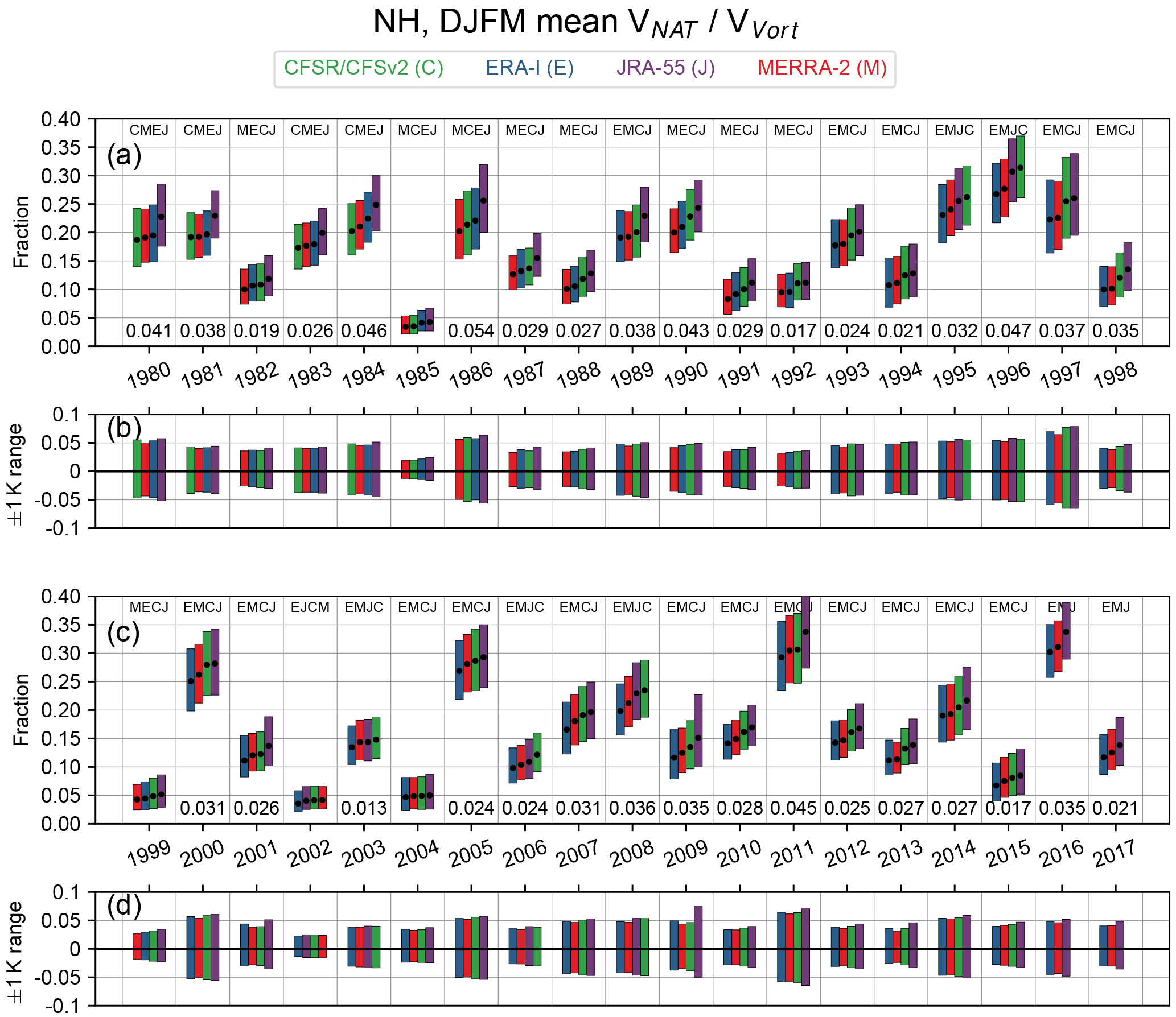
Potential polar processing volumes in the NH are much lower and much more variable than those in the SH. The NH fraction of vortex volume below TNAT (Fig. 16) shows values in the colder years that are comparable to those below Tice in the SH. The lowest values are seen in 1984/1985, 1998/1999, 2001/2002, and 2003/2004, which are all years with very early (mid-December to the beginning of January) major SSWs that profoundly affected the entire stratosphere, including strongly disrupting the lower stratospheric vortex (e.g., Manney et al., 1999, 2005b; Naujokat et al., 2002); in these years, the fractional volumes are near 0.03, as opposed to nearly 0.30 in the coldest years (e.g., 1996, 2011, 2016). The range of values from the PSC threshold temperature sensitivity tests varies from about ±0.02 in the warmest years up to over ±0.05 in the coldest years, with differences between reanalyses indicating some differences in horizontal temperature gradients (especially in, e.g., 1997, 2009, and 2011). The interannual variability is well represented in all of the reanalyses. The central values usually vary more between reanalyses in colder years; e.g., 1996 and 2011 stand out as showing wide ranges of about 0.045. Between 1992/1993 and 2016/2017, ERA-I tends to have the smallest vortex fractions. In contrast, JRA-55 tends to have the overall largest NAT vortex fractions, having the largest values for 32 of the 38 years, with many cases being noticeably offset from the other reanalyses. While many of the recent years show smaller ranges of central values than the early years, there is not a monotonic progression, so any trend towards better agreement is masked by the larger influence of specific interannually varying conditions that affect the PSC volumes.
We note that the results of intercomparisons of VPSC∕VVort outlined above are not very sensitive to the vortex volumes. When comparing these VPSC∕VVort results having VVort determined from the reanalyses' individual vortex areas to VPSC∕VVort calculated using the REM VVort (i.e., the reanalyses' VPSC divided by the REM VVort), the reanalysis magnitudes and orderings remain generally consistent. However, using the REM VVort does tend to decrease the inter-reanalysis spreads and the sensitivities to the ±1 K PSC temperature thresholds.

Figure 17Pixel plots of (a) vortex decay dates (see text for the definition) based on the REM of vortex area, and (b–e) the difference between the vortex decay dates in each of the reanalyses from the REM (as reanalysis − REM).
Figures 17 and 18 show pixel plots of the REM vortex decay dates and the differences from the other reanalyses (i.e., the reanalyses minus REM). For the SH, Fig. 17a shows that the vortex tends to decay fairly late in the year, and it does so earlier at the upper levels than at the lower levels; in other words, the vortex in the SH typically decays from the top down. The differences in decay dates among the reanalyses are generally less than 2 weeks; over 90 % of the differences are between ±7 days. The patterns of differences in each of the reanalyses generally follow their vortex area differences from the REM (which, while not shown, are very similar to differences shown in Fig. 13). That is, wherever the reanalyses have smaller/larger vortex areas than the REM, their vortices persist for less/more time. ERA-I shows some notable exceptions to this at levels above 700 K where its decay dates precede those of the REM by up to 14 days in the same region where ERA-I tended to have positive vortex area differences (see, e.g., 1980, 1981, 1987). Overall, because the differences in vortex area tend to be dominant and persistent, as shown in Fig. 13, so are the decay date differences, and thus there are no easily discernible changes in agreement over time.
Figure 18 shows that the NH vortex breakup is much more variable from year to year than that in the SH. Unlike the SH vortex, the NH vortex can decay nearly simultaneously over a wide range of levels (e.g., 1984 and 1999), or it can decay earlier at some low levels and later at higher levels (e.g., 2001 and 2009). Such variability in vortex decay is due to large variability induced by SSW disturbances to the vortex, as well as polar night jet oscillation events in which the middle and upper stratospheric vortex rapidly reforms following some major and minor disturbances (e.g., Hitchcock et al., 2013; Lawrence and Manney, 2018, and references therein). The reanalyses' differences from the REM are generally quite small; over 90 % of the differences are between ±4 days. With the exception of JRA-55, the reanalyses show no predominant patterns of differences (e.g., positive or negative bands). JRA-55 does seem to have a slightly more pronounced band of negative differences from about 620 to 700 K (with a band of small but positive differences above), in the same region where the JRA-55 vortex area differences tend to be the most negative (not shown directly but consistent with Fig. 14). There are also several outlier cases with absolute differences from the REM greater than 20 days (denoted by the white X symbols). Most of these cases are marginal scenarios when either the REM or the reanalyses' vortex areas oscillate above and below the specified 1 % of a hemisphere threshold at some levels, causing our algorithm to pick disparate decay dates. Many of these outlier cases occur at different singular levels and years in the reanalyses, but 460 K 2003/2004 does show up as a negative outlier in both CFSR/CFSv2 and JRA-55, while 660 K 2005/2006 shows up as a positive outlier in both CFSR/CFSv2 and ERA-I.
We have herein done an extensive intercomparison of diagnostics relevant to polar chemical processing among four recent full-input reanalyses, using the REM as a reference to compare CFSR/CFSv2, ERA-I, JRA-55, and MERRA-2. The diagnostics we compare are based on polar vortex and temperature conditions in the lower-to-middle stratosphere, and comprise measures of PSC formation and chlorine activation based on temperatures; vortex size, strength, and sunlight exposure; and additional diagnostics derived from those directly obtained from temperatures and vortex characteristics. They thus provide a thorough assessment of the reanalyses' representation of the potential for polar processing and ozone loss in both hemispheres. The main findings of our analyses are summarized in the following subsection.
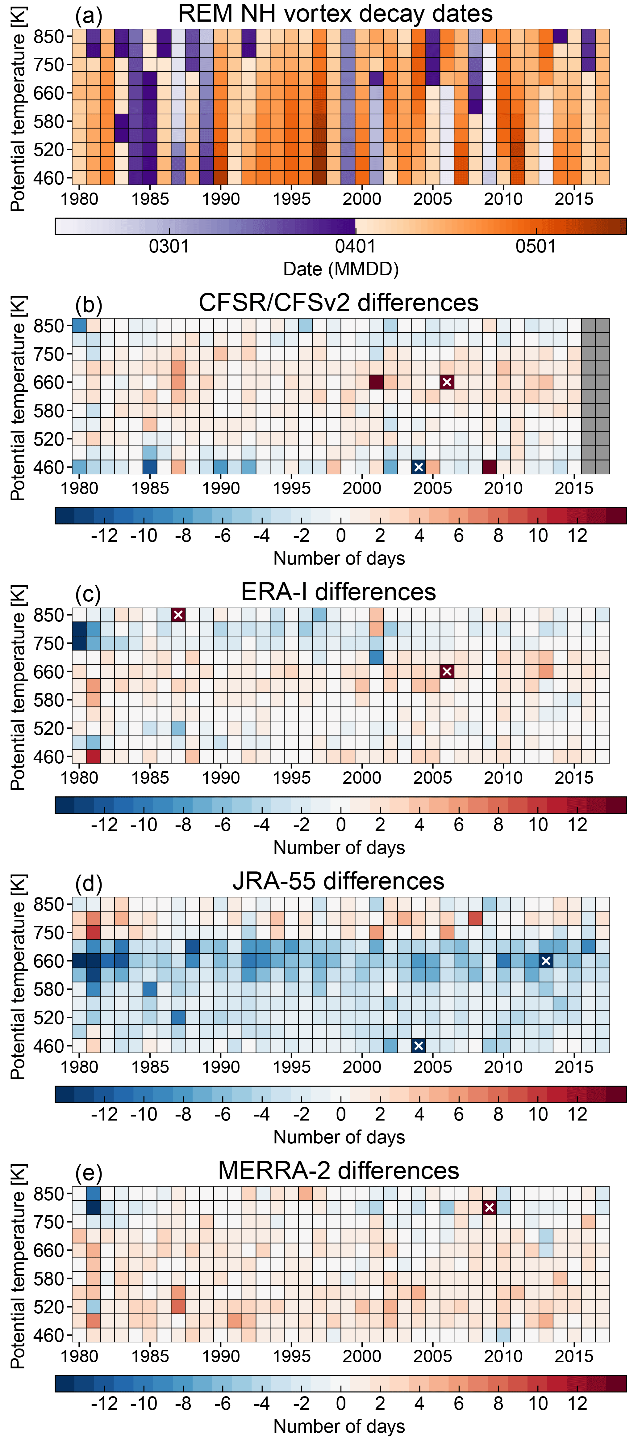
Figure 18As in Fig. 17 but for the NH. The color bar ranges are restricted to distinguish differences of a few days; differences whose magnitude greatly exceeds the range (by more than 7 days and thus differences with magnitude greater than 21 days) are marked with a white X symbol.
4.1 Summary
Temperature diagnostics related to polar processing converge towards better agreement in the SH over the period compared (from 1979 to present). In the period prior to ∼1999, reanalysis differences in minimum temperatures compared to the REM could be as large as ±3 K, particularly at pressures below 30 hPa; in years after, reanalysis minimum temperature differences from the REM decrease to within roughly ±0.5 K throughout the 120–10 hPa column. The reanalysis differences from the REM for SH areas with temperatures below the NAT PSC threshold (ANAT) show a similar and consistent shift, with differences among the reanalyses being as large as ±1.5 % of a hemisphere prior to ∼1999 but within ±0.5 % of a hemisphere thereafter. This shift toward better agreement in ∼1999 is seen as both a sudden decrease among the winter-averaged differences from the REM and as a sudden decrease in standard deviations of reanalysis minus REM differences, which is consistent with previous studies (e.g., Long et al., 2017) that show large improvements in zonal mean temperatures after the reanalyses transition from assimilating TOVS observations to including ATOVS. In the NH, the agreement among the reanalyses before ∼1999 was already much closer (generally within ±1.5 K from the REM for minimum temperatures but often within a much smaller margin at pressures greater than 30 hPa), but the average differences and standard deviations also decreased to a lesser extent thereafter. The structure of average differences, particularly before ∼1999, is varied among the reanalyses. MERRA-2 and ERA-I generally showed banded structures of average differences from the REM that changed signs with height prior to ∼1999. CFSR/CFSv2 tended to have average differences of the same sign throughout the 120–10 hPa column up until 1987, after which the differences switched signs (as in the case of minimum temperatures) or became more varied (as in the case of ANAT). The structure of average differences from the REM for JRA-55 was generally a bit more complicated than that in the other reanalyses but did show that the signs of the differences changed in the lower stratosphere between 100 and 30 hPa. The standard deviations of differences from the REM were quite consistent among the reanalyses; they increased with height (not necessarily monotonically), particularly at pressures lower than 30 hPa.
Differences from the REM among the reanalyses for SH MPVGs showed a similar convergence toward better agreement as did the temperature diagnostics. Differences from the REM were within roughly ±2.5 PVGUs prior to ∼1999 but within ±1 PVGU after. The standard deviations of the SH differences increased with height to values that were commonly above 2 PVGUs, particularly at isentropic levels above 600 K; after 1999, these standard deviations decreased in magnitude, but the pattern of values increasing with height remained consistent. In these cases the differences from the REM for SH MPVGs were consistently negative across all years for CFSR/CFSv2, while those for JRA-55 were consistently positive. ERA-I and MERRA-2 had banded structures of differences similar to those in the SH temperature diagnostics that mostly disappeared after ∼1999. In the case of NH MPVGs, differences remained largely constant over time and potential temperature levels, generally being within ±1.5 PVGUs of the REM with standard deviations that increased with height. Here, again, CFSR/CFSv2 had average differences from the REM that were consistently negative, while JRA-55 was consistently positive. Differences from the REM in sunlit vortex area across the reanalyses in both hemispheres remained relatively constant over time, and they overall followed differences in the raw vortex areas.
In the SH, all the reanalyses showed similar magnitudes and temperature threshold sensitivities in the winter mean volume of air (as a fraction of vortex volume) below ice PSC thresholds. In the NH, the winter mean volume of air below NAT PSC thresholds varied much more from year to year, and the differences among the reanalyses and sensitivities to the temperature offsets were much larger percentages of the actual derived values. These characteristics are in many ways to be expected, since SH winters are much more consistent from year to year than NH winters; thus, even though the individual temperature polar processing diagnostics showed much larger average differences and standard deviations in the SH, the aggregation of the full winter seasons in the winter mean VPSC∕VVort led to more consistent results. For the vortex decay dates, the reanalyses' differences from the REM generally followed their differences from the REM in vortex area (and as a result, sunlit vortex area) in that wherever the reanalyses had larger/smaller vortex areas, they also had later/earlier vortex decay dates. The agreement among the reanalyses for vortex decay dates was generally best in the NH, despite there being some marginal cases with large differences due to vortex disturbances.
4.2 Implications
The results shown herein illustrate some implications that may be expected for polar processing studies using reanalysis temperatures and PV in the stratosphere. These implications will generally depend on the hemisphere in question and the details of the study. For example, the derived diagnostics in Sect. 3.3 demonstrate that in the aggregate most SH winters in the satellite era are quite similar, and that the sensitivities to different PSC temperature thresholds are consistent among the reanalyses. However, the differences shown in Sect. 3.1 indicate that differences can depend strongly on the levels and years examined, especially prior to 1999 before the assimilation of AMSU data in the reanalyses. Thus, studies that discuss SH winter conditions in aggregate are less likely to be affected than detailed studies (e.g., those making use of nudged and specified dynamics models, and/or Lagrangian transport models), whose conclusions could be significantly altered by the details of how, when, and where the temperatures differ among the reanalyses. In contrast, for the NH, Sect. 3.1 showed that temperature diagnostic differences were relatively small among the reanalyses, but the results in Sect. 3.3 showed that the winter-mean derived diagnostics vary widely between reanalyses in some cases, and can be highly sensitive to the specific temperature thresholds used. Clearly polar processing potential is often much smaller in the NH than in the SH, and thus conclusions based on the often marginal conditions of the NH are much more likely to be affected by small differences among the reanalyses. Thus, both detailed and aggregate studies of NH polar processing could in some cases be markedly affected by differences among the reanalyses. However, all of the reanalyses do show similar interannual variations among the derived diagnostics, and thus for purposes of putting some NH winters into the context of others (e.g., comparing how cold some are relative to others), any of the reanalyses would give similar results. The extent to which different kinds of studies of NH and/or SH polar processing may be affected is beyond the scope of this paper, but work is in progress within S-RIP to explore some of these implications.
It is difficult to assess the potential implications of differences among the reanalyses in the vortex diagnostics. Since MERRA-2 is the only reanalysis that provides PV fields on its model levels, we have applied the strategy we think other data users requiring PV on model levels would use, which was to derive PV from each reanalysis using their available model level products. Thus, it is important to recognize that the vortex diagnostics used herein are derived from PV fields that are calculated from the different reanalyses in different ways, which makes it problematic to assess whether and the extent to which the reanalysis differences are due to differences in such factors as the calculations, dynamics, and vertical and/or horizontal resolution. Because MERRA-2 includes PV calculated within its DAS, we generally consider MERRA-2 PV to be more consistent and complete than the PV fields derived from the other reanalyses' model level data. Despite these complicating factors, our treating each of the reanalyses equally (same procedure for calculating MPVGs, and using each of the reanalyses' climatological MPVGs to define vortex edges) allows us to draw some useful conclusions. While there were some small indications of convergence toward better agreement in MPVGs for both hemispheres among some reanalyses (see Sect. 3.2), there were primarily persistent differences in SVA. Given the combination of differences in MPVGs and SVA (and raw vortex area), the results shown here indicate that there are some inherent differences in the PV fields that lead to somewhat disparate equivalent latitude mappings, which in some cases could alter conclusions drawn about transport barriers and trace gases in equivalent latitude coordinates. It is also possible that results for the SH were contaminated by the presence of double-peaked (bifurcated) PV gradients (e.g., Conway et al., 2018) that could have different magnitudes or structures among the reanalyses.
4.3 Recommendations
All of the reanalyses used here represent very large improvements over those commonly used a decade ago, and with those improvements comes much closer agreement in the polar processing diagnostics presented here. The older reanalyses, especially ERA-40 and NCEP/NCAR and NCEP/DOE, have long been obsolete and are not recommended for studies focused on polar processing and the stratosphere in general (see Fujiwara et al., 2017, and references therein). Any of the modern reanalyses evaluated herein are much better choices for polar processing studies as they all provide more accurate and similar representations of interannual variability in polar processing diagnostics in both hemispheres.
In general, it is always better to use more than one reanalysis, even for studies involving recent winters where it can reasonably be expected that differences among the reanalyses will be small. One of the best ways to express uncertainty in results is using multiple reanalyses, and explicitly showing and discussing how they agree/disagree, and whether any differences affect the findings; this is especially important for diagnostics that cannot be compared with observations. As previously shown by Lawrence et al. (2015) for polar processing diagnostics, and Long et al. (2017) for zonal means, our intercomparisons (see particularly Figs. 4–5 and 7–8) show that there are substantial (especially large in the SH) changes in temperature-based diagnostics that are clearly related to changes in assimilated data inputs among the reanalyses. Since many of the major changes in data inputs are made at approximately the same time in each reanalysis, the agreement or lack thereof between the reanalyses does not provide the information to assess the degree to which these changes are caused by changes to the assimilated observations. We thus emphasize here that reanalysis temperatures, especially in the Antarctic, are not generally suitable for assessment of trends in temperature-based diagnostics; use of reanalyses in trend studies should be regarded with skepticism and only attempted after rigorous assessment of the relationships of temperature changes to observations assimilated (which, to our knowledge, has not been done for most of the reanalyses considered here); were such a study to be done, agreement among multiple reanalyses would in addition be required to consider any trends robust.
When using multiple reanalyses, it is important to treat them as fairly and equally as possible to reduce the uncertainty in sources of differences. For example, using one reanalysis with data on model levels and another one with data on pressure levels is not recommended. It is also important to be clear whether and how fields/quantities are derived from the products provided by the reanalyses, as we have done herein with PV. Until and unless reanalysis centers provide standard sets of products on standardized isobaric and isentropic levels, users of reanalysis data will generally be best served by using model data to vertically interpolate and derive fields as needed. Numerous evaluations of reanalyses for S-RIP are finding, as we have here, that it would be valuable to have PV on model levels available in future reanalyses.
With regard to more specific polar processing applications, we also recommend that trends, correlations, and/or other similar analyses of diagnostics that assess low temperatures aggregated over winter months, seasons, and/or vertical levels in the NH polar region be performed with caution. Figure 16 demonstrates that there is non-negligible interannual variability in the sensitivity to the specific temperature values chosen to represent NAT PSC thresholds that are used to calculate the volume of air below NAT thresholds in the NH, especially relative to the SH (Fig. 15) in which we used the lower ice PSC thresholds. The vortex diagnostics in Sect. 3.2 show some differences that appear to be related to biases between PV in the reanalyses, arguing for careful assessment of the sensitivity of vortex diagnostics to exact PV values. Because many of the diagnostics that are most informative about lower stratospheric polar chemical processing cannot be readily validated by comparison with data, the comparison of reanalyses is a powerful tool for assessing robustness and uncertainty in these diagnostics.
The HNO3 and H2O profiles used for the calculation of NAT and ice PSC thresholds are given in Table A1. These values were derived from Upper Atmosphere Research Satellite (UARS) measurements from the Cryogenic Limb Array Etalon Spectrometer for HNO3 and Microwave Limb Sounder for H2O, by averaging values for December/January 1991/1992 and 1992/1993, as described by Manney et al. (2003, 2005a). The values are thus close to climatological values for the NH and for the SH during early winter. The values are defined at six levels per decade in pressure (standard UARS levels) and interpolated to the same 12-level-per-decade pressures that the reanalyses are interpolated to. Approximately corresponding isentropic surfaces were estimated by averaging climatological (Fleming et al., 1990) temperature profiles for January, April, July, and October (the solstice and equinox months) at ±70, ±50, and ±10∘ latitude; the potential temperatures thus derived are then adjusted to “nice” values (i.e., to the nearest 5 or 10 K depending on the spacing of potential temperature levels at that height. The pressure levels used for the analysis, their approximately corresponding potential temperature levels, and the NAT and ice PSC thresholds calculated from them are listed in Table A2. These HNO3 and H2O profiles, and the PSC thresholds derived from them, may not be the most appropriate for studies requiring precise estimates of the PSC thresholds and PSC potential throughout the winter. Especially in the SH, denitrification and dehydration can significantly change the profiles of HNO3 and H2O away from the climatology. Furthermore, using the same PSC thresholds from pressure surfaces on potential temperature surfaces is an additional approximation that tends to overestimate the size of regions with low temperatures. Regardless, these values are appropriate for defining regions and periods of time when polar processing can take place, and for understanding the differences among reanalyses.
Table A1HNO3 and H2O values for PSC threshold calculation. Pressure values are rounded to nearest integer.
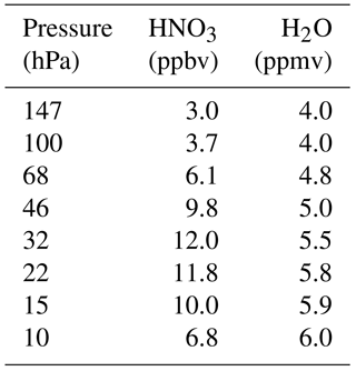
Table A2Pressure levels, approximately corresponding potential temperature levels, and the NAT and ice PSC thresholds calculated from Table A1. Pressure values are rounded to the nearest integer; NAT and ice PSC thresholds are rounded to the nearest tenth of a Kelvin.
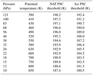
The datasets used/produced are publicly available, as follows:
-
MERRA-2: https://disc.sci.gsfc.nasa.gov/uui/datasets?keywords=\%22MERRA-2\%22 (last access: 22 August 2018)
-
ERA-I: http://apps.ecmwf.int/datasets/ (last access: 19 September 2018)
-
JRA-55: through NCAR RDA at https://doi.org/10.5065/D6HH6H41 (last access: 15 February 2018)
-
CFSR/CFSv2 model level data: available upon request from Karen H. Rosenlof (karen.h.rosenlof@noaa.gov)
-
Polar processing diagnostic products: contact Zachary D. Lawrence (zachary.lawrence@student.nmt.edu)
ZDL and GLM designed the study. ZDL did the analysis. KW provided expertise and guidance on the reanalysis datasets. ZDL and GLM wrote the discussion paper and KW commented on and edited it; ZDL, KW, and GLM revised the paper.
The authors declare no competing interests.
This article is part of the special issue “The SPARC Reanalysis Intercomparison Project (S-RIP) (ACP/ESSD inter-journal SI)”. It is not associated with a conference.
We thank the Microwave Limb Sounder team at JPL, especially Brian W. Knosp and Ryan A. Fuller, for
computational, data processing, management, and analysis support;
Will McCarty and Larry Coy of the GMAO for helpful comments; NASA's GMAO, ECMWF, JMA, and NCEP
for providing their assimilated data products;
Amy Butler, Jeremiah Sjoberg, Craig Long, Sean Davis, Henry L. Miller, and Karen Rosenlof for
processing and providing the model level CFSR/CFSv2 data; and Simon Chabrillat and an
anonymous reviewer for their constructive and helpful comments that improved this paper.
GLM and ZDL were supported by the JPL Microwave Limb Sounder team under JPL subcontracts to
NWRA and NMT; KW was supported by the NASA Modeling, Analysis and Prediction (MAP) program,
which also provides support for MERRA and MERRA-2.
Edited by: William Lahoz
Reviewed by: Simon Chabrillat and one anonymous referee
Ajtić, J., Connor, B. J., Randall, C. E., Lawrence, B. N., Bodeker, G. E., Rosenfield, J. E., and Heuff, D. N.: Antarctic air over New Zealand following vortex breakdown in 1998, Ann. Geophys., 21, 2175–2183, 2003. a, b
Ajtić, J., Connor, B. J., Lawrence, B. N., Bodeker, G. E., Hoppel, K. W., Rosenfield, J. E., and Heuff, D. N.: Dilution of the Antarctic ozone hole into southern midlatitudes, 1998–2000, J. Geophys. Res., 109, D17107, https://doi.org/10.1029/2003JD004500, 2004. a, b
Albers, J. R. and Nathan, T. R.: Ozone Loss and Recovery and the Preconditioning of Upward-Propagating Planetary Wave Activity, J. Atmos. Sci., 70, 3977–3994, https://doi.org/10.1175/JAS-D-12-0259.1, 2013. a
Andrews, D. G.: Some comparisons between the middle atmosphere dynamics for the southern and northern hemispheres, Pure Appl. Geophys., 130, 213–232, 1989. a
Bernhard, G., Manney, G., Fioletov, V., Grooß, J.-U., Heikkila, A., Johnson, B., Koslela, T., Lakkala, K., Müller, R., Myhre, C., and Rex, M.: [The Arctic] Ozone and UV Radiation, [in “State of the Climate in 2011”.], B. Am. Meteorol. Soc., 93, S129–S132, 2012. a
Bloom, S. C., Takacs, L. L., da Silva, A. M., and Ledvina, D.: Data assimilation using incremental analysis updates, Mon. Weather Rev., 124, 1256–1271, 1996. a
Boccara, G., Hertzog, A., Basdevant, C., and Vial, F.: Accuracy of NCEP/NCAR reanalyses and ECMWF analyses in the lower stratosphere over Antarctica in 2005, J. Geophys. Res., 113, d20115, https://doi.org/10.1029/2008JD010116, 2008. a
Bosilovich, M., Akella, S., Coy, L., Cullather, R., Draper, C., Gelaro, R., Kovach, R., Liu, Q., Molod, A., Norris, P., Wargan, K., Chao, W., Reichle, R., Takacs, L., Vikhliaev, Y., Bloom, S., Collow, A., Firth, S., Labow, G., Partyka, G., Pawson, S., Reale, O., Schubert, S. D., and Suarez, M.: MERRA-2: Initial Evaluation of the Climate, Series on Global Modeling and Data Assimilation, NASA/TM-2015-104606, Vol. 43, NASA, 2015. a
Bosilovich, M. G., Lucchesi, R., and Suarez, M.: MERRA-2: File Specification, Office Note 9, GMAO Office Note, 73 pp, available at: https://gmao.gsfc.nasa.gov/pubs/docs/Bosilovich785.pdf (last access: 13 September 2018), 2016. a
Butchart, N. and Remsberg, E. E.: The area of the stratospheric polar vortex as a diagnostic for tracer transport on an isentropic surface, J. Atmos. Sci., 43, 1319–1339, 1986. a
Conway, J., Bodeker, G., and Cameron, C.: Bifurcation of potential vorticity gradients across the Southern Hemisphere stratospheric polar vortex, Atmos. Chem. Phys., 18, 8065–8077, https://doi.org/10.5194/acp-18-8065-2018, 2018. a
Davies, S., Chipperfield, M. P., Carslaw, K. S., Sinnhuber, B.-M., Anderson, J. G., Stimpfle, R. M., Wilmouth, D. M., Fahey, D. W., Popp, P. J., Richard, E. C., von der Gathen, P., Jost, H., and Webster, C. R.: Modeling the effect of denitrification on Arctic ozone depletion during winter 1999/2000, J. Geophys. Res., 108, 8322, https://doi.org/10.1029/2001JD000445, 2003. a
Dee, D. P., Uppala, S. M., Simmons, A. J., Berrisford, P., Poli, P., Kobayashi, S., Andrae, U., Balmaseda, M. A., Balsamo, G., Bauer, P., Bechtold, P., Beljaars, A. C. M., van de Berg, L., Bidlot, J., Bormann, N., Delsol, C., Dragani, R., Fuentes, M., Geer, A. J., Haimberger, L., Healy, S. B., Hersbach, H., Hólm, E. V., Isaksen, L., Kållberg, P., Köhler, M., Matricardi, M., McNally, A. P., Monge-Sanz, B. M., Morcrette, J.-J., Park, B.-K., Peubey, C., de Rosnay, P., Tavolato, C., Thépaut, J.-N., and Vitart, F.: The ERA-Interim reanalysis: configuration and performance of the data assimilation system, Q. J. Roy. Meteorol. Soc., 137, 553–597, 2011. a
DiCiccio, T. J. and Efron, B.: Bootstrap confidence intervals, Statist. Sci., 11, 189–228, https://doi.org/10.1214/ss/1032280214, 1996. a
Dunkerton, T. J. and Delisi, D. P.: Evolution of potential vorticity in the winter stratosphere of January–February 1979, J. Geophys. Res., 91, 1199–1208, 1986. a
Ebita, A., Kobayashi, S., Ota, Y., Moriya, M., Kumabe, R., Onogi, K., Harada, Y., Yasui, S., Miyaoka, K., Takahashi, K., Kamahori, H., Kobayashi, C., Endo, H., Soma, M., Oikawa, Y., and Ishimizu, T.: The Japanese 55-year Reanalysis “JRA-55”: An interim report, SOLA, 7, 149–152, 2011. a
Feng, W., Chipperfield, M. P., Roscoe, H. K., Remedios, J. J., Waterfall, A. M., Stiller, G. P., Glatthor, N., Höpfner, M., and Wang, D.-Y.: Three-dimensional model study of the Antarctic ozone hole in 2002 and comparison with 2000, J. Atmos. Sci., 62, 822–837, 2005. a, b
Fleming, E., Chandra, S., Barnett, J. J., and Corney, M.: Zonal mean temperature, pressure, zonal wind and geopotential height as functions of latitude, Adv. Sp. Res., 10, 11–53, 1990. a
Forster, P. M. and Shine, K. P.: Radiative forcing and temperature trends from stratospheric ozone changes, J. Geophys. Res., 102, 10841–10855, 1997. a
Fujiwara, M., Wright, J. S., Manney, G. L., Gray, L. J., Anstey, J., Birner, T., Davis, S., Gerber, E. P., Harvey, V. L., Hegglin, M. I., Homeyer, C. R., Knox, J. A., Krüger, K., Lambert, A., Long, C. S., Martineau, P., Monge-Sanz, B. M., Santee, M. L., Tegtmeier, S., Chabrillat, S., Tan, D. G. H., Jackson, D. R., Polavarapu, S., Compo, G. P., Dragani, R., Ebisuzaki, W., Harad̃a, Y., Kobayashi, C., McCarty, W., Onogi, K., Pawson, S., Simmons, A., Wargan, K., Whitaker, J. S., and Zou, C.-Z.: Introduction to the SPARC Reanalysis Intercomparison Project (S-RIP) and overview of the reanalysis systems, Atmos. Chem. Phys., 17, 1417–1452, https://doi.org/10.5194/acp-17-1417-2017, 2017. a, b, c, d, e, f, g, h, i, j, k, l
Gelaro, R., McCarty, W., Suárez, M. J., Todling, R., Molod, A., Takacs, L., Randles, C. A., nov, A. D., Bosilovich, M. G., Reichle, R., Wargan, K., Coy, L., Cullather, R., Draper, C., Akella, S., Buchard, V., Conaty, A., da Silva, A. M., Gu, W., Kim, G.-K., Koster, R., Lucchesi, R., Merkova, D., N, J. E. N., Partyka, G., Pawson, S., Putman, W., Rienecker, M., Schubert, S. D., Sienkiewicz, M., and Zhao, B.: The Modern-Era Retrospective Analysis for Research and Applications, Version-2 (MERRA-2), J. Climate, 30, 5419–5454, https://doi.org/10.1175/JCLI-D-16-0758.1, 2017. a
Global Modeling and Assimilation Office (GMAO): MERRA-2 inst3_3d_asm_Nv: 3d, 3-Hourly, Instantaneous, Model-Level, Assimilation, Assimilated Meteorological Fields V5.12.4, Greenbelt, MD, USA, Goddard Earth Sciences Data and Information Services Center (GES DISC), access: 1 November 2015, https://doi.org/10.5067/WWQSXQ8IVFW8, 2015. a
Global Modeling and Assimilation Office (GMAO): Use of MERRA-2 for Atmospheric Chemistry and Transport Studies, available at: https://gmao.gsfc.nasa.gov/reanalysis/MERRA-2/docs/ANAvsASM.pdf (last access: 13 September 2018), 2017. a
Gobiet, A., Kirchengast, G., Manney, G. L., Borsche, M., Retscher, C., and Stiller, G.: Retrieval of temperature profiles from CHAMP for climate monitoring: intercomparison with Envisat MIPAS and GOMOS and different atmospheric analyses, Atmos. Chem. Phys., 7, 3519–3536, https://doi.org/10.5194/acp-7-3519-2007, 2007. a
Hanson, D. and Mauersberger, K.: Laboratory studies of the nitric acid trihydrate: Implications for the south polar stratosphere, Geophys. Res. Lett., 15, 855–858, 1988. a, b, c
Hegglin, M. I., Boone, C. D., Manney, G. L., and Walker, K. A.: A global view of the extratropical tropopause transition layer (ExTL) from Atmospheric Chemistry Experiment Fourier Transform Spectrometer O3, H2O, and CO, J. Geophys. Res., 114, D00B11, https://doi.org/10.1029/2008JD009984, 2009. a
Hitchcock, P., Shepherd, T. G., and Manney, G. L.: Statistical characterization of Arctic polar-night jet oscillation events, J. Climate, 26, 2096–2116, 2013. a
Hoffmann, L. and Alexander, M. J.: Retrieval of stratospheric temperatures from Atmospheric Infrared Sounder radiance measurements for gravity wave studies, J. Geophys. Res., 114, D07105, https://doi.org/10.1029/2008JD011241, 2009. a
Hoffmann, L., Hertzog, A., Rößler, T., Stein, O., and Wu, X.: Intercomparison of meteorological analyses and trajectories in the Antarctic lower stratosphere with Concordiasi superpressure balloon observations, Atmos. Chem. Phys., 17, 8045–8061, https://doi.org/10.5194/acp-17-8045-2017, 2017. a, b, c
Huck, P. E., McDonald, A. J., Bodeker, G. E., and Struthers, H.: Interannual variability in Antarctic ozone depletion controlled by planetary waves and polar temperatures, Geophys. Res. Lett., 32, L13819, https://doi.org/10.1029/2005GL022943, 2005. a
Knox, J. A.: On converting potential temperature to altitude in the middle atmosphere, Eos Trans. AGU, 79, 376, 1998. a
Knudsen, B. M., Rosen, J. M., Kjome, N. T., and Whitten, A. T.: Comparison of analyzed stratospheric temperatures and calculated trajectories with long-duration balloon data, J. Geophys. Res., 101, 19137–19145, 1996. a
Knudsen, B. M., Pommereau, J.-P., Garnier, A., Nunez-Pinharanda, M., Denis, L., Letrenne, G., Durand, M., and Rosen, J. M.: Comparison of stratospheric air parcel trajectories based on different meteorological analyses, J. Geophys. Res., 106, 3415–3424, 2001. a
Knudsen, B. M., Rosen, J. M., Kjome, N. T., and Whitten, A. T.: Accuracy of analyzed stratospheric temperatures in the winter Arctic vortex from infrared Montgolfier long-duration balloon flights 2. Results, J. Geophys. Res., 107, D001329, https://doi.org/10.1029/2001JD001329, 2002. a
Kobayashi, S., Ota, Y., Harada, Y., Ebita, A., Moriya, M., Onoda, H., Onogi, K., Kamahori, H., Kobayashi, C., Endo, H., Miyaoka, K., and Takahashi, K.: The JRA-55 Reanalysis: General Specification and Basic Characteristics, J. Meteor. Soc. JPN, 93, 5–48, https://doi.org/10.2151/jmsj.2015-001, 2015. a
Lacis, A., Wuebbles, D. J., and Logan, J. A.: Radiative forcing of climate by changes in the vertical distribution of ozone, J. Geophys. Res., 95, 9971–9981, 1990. a
Lahiri, S.: Resampling Methods for Dependent Data, Springer Series in Statistics, Springer, 2003. a
Lambert, A. and Santee, M. L.: Accuracy and precision of polar lower stratospheric temperatures from reanalyses evaluated from A-Train CALIOP and MLS, COSMIC GPS RO, and the equilibrium thermodynamics of supercooled ternary solutions and ice clouds, Atmos. Chem. Phys., 18, 1945–1975, https://doi.org/10.5194/acp-18-1945-2018, 2018. a, b, c, d, e
Lawrence, Z. D. and Manney, G. L.: Characterizing Stratospheric Polar Vortex Variability With Computer Vision Techniques, J. Geophys. Res.-Atmos., 123, 1510–1535, https://doi.org/10.1002/2017JD027556, 2018. a, b, c
Lawrence, Z. D., Manney, G. L., Minschwaner, K., Santee, M. L., and Lambert, A.: Comparisons of polar processing diagnostics from 34 years of the ERA-Interim and MERRA reanalyses, Atmos. Chem. Phys., 15, 3873–3892, https://doi.org/10.5194/acp-15-3873-2015, 2015. a, b, c, d, e, f, g, h, i
Levine, J. G., Braesicke, P., Harris, N. R., Savage, N. H., and Pyle, J. A.: Pathways and timescales for troposphere-to-stratosphere transport via the tropical tropopause layer and their relevance for very short lived substances, J. Geophys. Res., 112, D04308, https://doi.org/10.1029/2005JD006940, 2007. a
Livesey, N. J., Read, W. G., Wagner, P. A., Froidevaux, L., Lambert, A., Manney, G. L., Millán Valle, L. F., Pumphrey, H. C., Santee, M. L., Schwartz, M. J., Wang, S., Fuller, R. A., Jarnot, R. F., Knosp, B. W., and Martinez, E.: EOS MLS Version 4.2x Level 2 data quality and description document, Tech. rep., JPL, available at: http://mls.jpl.nasa.gov/ (last access: 13 September 2018), 2015. a
Long, C. S., Fujiwara, M., Davis, S., Mitchell, D. M., and Wright, C. J.: Climatology and Interannual Variability of Dynamic Variables in Multiple Reanalyses Evaluated by the SPARC Reanalysis Intercomparison Project (S-RIP), Atmos. Chem. Phys., 17, 14593–14629, 2017. a, b, c, d, e, f, g, h, i
Long, C. S., Fujiwara, M., Davis, S., Mitchell, D., and Wright, C.: SPARC Reanalysis Intercomparison Project (S-RIP) Final Report. Chapter 3: Overview of Winds and Temperatures, SPARC, in preparation, 2018. a, b
Manney, G. L. and Lawrence, Z. D.: The major stratospheric final warming in 2016: dispersal of vortex air and termination of Arctic chemical ozone loss, Atmos. Chem. Phys., 16, 15371–15396, https://doi.org/10.5194/acp-16-15371-2016, 2016. a, b
Manney, G. L., Zurek, R. W., Gelman, M. E., Miller, A. J., and Nagatani, R.: The anomalous Arctic lower stratospheric polar vortex of 1992–1993, Geophys. Res. Lett., 21, 2405–2408, 1994. a
Manney, G. L., Swinbank, R., Massie, S. T., Gelman, M. E., Miller, A. J., Nagatani, R., O'Neill, A., and Zurek, R. W.: Comparison of U. K. Meteorological Office and U. S. National Meteorological Center stratospheric analyses during northern and southern winter, J. Geophys. Res., 101, 10311–10334, 1996. a
Manney, G. L., Lahoz, W. A., Swinbank, R., O'Neill, A., Connew, P. M., and Zurek, R. W.: Simulation of the December 1998 stratospheric major warming, Geophys. Res. Lett., 26, 2733–2736, 1999. a
Manney, G. L., Sabutis, J. L., Pawson, S., Santee, M. L., Naujokat, B., Swinbank, R., Gelman, M. E., and Ebisuzaki, W.: Lower stratospheric temperature differences between meteorological analyses in two cold Arctic winters and their impact on polar processing studies, J. Geophys. Res., 108, 8328, https://doi.org/10.1029/2001JD001149, 2003. a, b
Manney, G. L., Allen, D. R., Krüger, K., Naujokat, B., Santee, M. L., Sabutis, J. L., Pawson, S., Swinbank, R., Randall, C. E., Simmons, A. J., and Long, C.: Diagnostic Comparison of Meteorological Analyses during the 2002 Antarctic Winter, Mon. Weather Rev., 133, 1261–1278, 2005a. a, b, c
Manney, G. L., Krüger, K., Sabutis, J. L., Sena, S. A., and Pawson, S.: The remarkable 2003–2004 winter and other recent warm winters in the Arctic stratosphere since the late 1990s, J. Geophys. Res., 110, D04107, https://doi.org/10.1029/2004JD005367, 2005b. a, b, c
Manney, G. L., Santee, M. L., Livesey, N. J., Froidevaux, L., Read, W. G., Pumphrey, H. C., Waters, J. W., and Pawson, S.: EOS Microwave Limb Sounder observations of the Antarctic polar vortex breakup in 2004, Geophys. Res. Lett., 32, L12811, https://doi.org/10.1029/2005GL022823, 2005c. a
Manney, G. L., Daffer, W. H., Zawodny, J. M., Bernath, P. F., Hoppel, K. W., Walker, K. A., Knosp, B. W., Boone, C., Remsberg, E. E., Santee, M. L., Harvey, V. L., Pawson, S., Jackson, D. R., Deaver, L., McElroy, C. T., McLinden, C. A., Drummond, J. R., Pumphrey, H. C., Lambert, A., Schwartz, M. J., Froidevaux, L., McLeod, S., Takacs, L. L., Suarez, M. J., Trepte, C. R., Cuddy, D. C., Livesey, N. J., Harwood, R. S., and Waters, J. W.: Solar occultation satellite data and derived meteorological products: Sampling issues and comparisons with Aura Microwave Limb Sounder, J. Geophys. Res., 112, D24S50, https://doi.org/10.1029/2007JD008709, 2007. a
Manney, G. L., Santee, M. L., Rex, M., Livesey, N. J., Pitts, M. C., Veefkind, P., Nash, E. R., Wohltmann, I., Lehmann, R., Froidevaux, L., Poole, L. R., Schoeberl, M. R., Haffner, D. P., Davies, J., Dorokhov, V., Gernandt, H., Johnson, B., Kivi, R., Kyrö, E., Larsen, N., Levelt, P. F., Makshtas, A., McElroy, C. T., Nakajima, H., Parrondo, M. C., Tarasick, D. W., von der Gathen, P., Walker, K. A., and Zinoviev, N. S.: Unprecedented Arctic Ozone Loss in 2011, Nature, 478, 469–475, 2011. a, b, c
Manney, G. L., Hegglin, M. I., Lawrence, Z. D., Wargan, K., Millán, L. F., Schwartz, M. J., Santee, M. L., Lambert, A., Pawson, S., Knosp, B. W., Fuller, R. A., and Daffer, W. H.: Reanalysis comparisons of upper tropospheric-lower stratospheric jets and multiple tropopauses, Atmos. Chem. Phys., 17, 11541–11566, https://doi.org/10.5194/acp-17-11541-2017, 2017. a
McIntyre, M. E. and Palmer, T. N.: The “surf zone” in the stratosphere, J. Atmos. Terr. Phys., 46, 825–849, 1984. a
Molod, A., Takacs, L., Suarez, M., and Bacmeister, J.: Development of the GEOS-5 atmospheric general circulation model: evolution from MERRA to MERRA2, Geosci. Model Dev., 8, 1339–1356, https://doi.org/10.5194/gmd-8-1339-2015, 2015. a
Nash, E. R., Newman, P. A., Rosenfield, J. E., and Schoeberl, M. R.: An objective determination of the polar vortex using Ertel's potential vorticity, J. Geophys. Res., 101, 9471–9478, 1996. a, b
Naujokat, B., Krüger, K., Matthes, K., Hoffmann, J., Kunze, M., and Labitzke, K.: The early major warming in December 2001 – exceptional?, Geophys. Res. Lett., 29, 2023, https://doi.org/10.1029/2002GL015316, 2002. a
Newman, P. A., Kawa, S. R., and Nash, E. R.: On the size of the Antarctic ozone hole, Geophys. Res. Lett., 31, L21104, https://doi.org/10.1029/2004GL020596, 2004. a
Pawson, S., Krüger, K., Swinbank, R., Bailey, M., and O'Neill, A.: Intercomparison of two stratospheric analyses: Temperatures relevant to polar stratospheric cloud formation, J. Geophys. Res., 104, 2041–2050, 1999. a
Pazmino, A. F., Godin-Beekmann, S., Ginzburg, M., Bekki, S., Hauchecorne, A., Piacentini, R. D., and Quel, E. J.: Impact of Antarctic polar vortex occurrences on total ozone and UVB radiation at southern Argentinean and Antarctic stations during 1997–2003 period, J. Geophys. Res., 110, D03103, https://doi.org/10.1029/2004JD005304, 2005. a, b
Politis, D. N. and Romano, J. P.: The Stationary Bootstrap, J. Am. Stat. Assoc., 89, 1303–1313, 1994. a
Polvani, L. M., Waugh, D. W., Correa, G. J., and Son, S.-W.: Stratospheric ozone depletion: The main driver of twentieth-century atmospheric circulation changes in the Southern Hemisphere, J. Climate, 24, 795–812, 2011. a
Rex, M., Salawitch, R. J., Gathen, P., Harris, N. R., Chipperfield, M. P., and Naujokat, B.: Arctic ozone loss and climate change, Geophys. Res. Lett., 31, L04116, https://doi.org/10.1029/2003GL018844, 2004. a
Rex, M., Salawitch, R. J., Deckelmann, H., von der Gathen, P., Harris, N. R. P., Chipperfield, M. P., Naujokat, B., Reimer, E., Allart, M., Andersen, S. B., Bevilacqua, R., Braathen, G. O., Claude, H., Davies, J., De Backer, H., Dier, H., Dorokhov, V., Fast, H., Gerding, M., Godin-Beekmann, S., Hoppel, K., Johnson, B., Kyrö, E., Litynska, Z., Moore, D., Nakane, H., Parrondo, M. C., Risley, A. D., Skrivankova, P., Stübi, R., Viatte, P., Yushkov, V., and Zerefos, C.: Arctic winter 2005: Implications for stratospheric ozone loss and climate change, Geophys. Res. Lett., 33, L23808, https://doi.org/10.1029/2006GL026731, 2006. a
Rienecker, M. M., Suarez, M. J., Gelaro, R., Todling, R., Bacmeister, J., Liu, E., Bosilovich, M. G., Schubert, S. D., Takacs, L., Kim, G., Bloom, S., Chen, J., Collins, D., Conaty, A., da Silva, A., Gu, W., Joiner, J., Koster, R. D., Lucchesi, R., Molod, A., Owens, T., Pawson, S., Pegion, P., Redder, C. R., Reichle, R., Robertson, F. R., Ruddick, A. G., Sienkiewicz, M., and Woollen, J.: MERRA: NASA's Modern-Era Retrospective Analysis for Research and Applications, J. Climate, 24, 3624–3648, 2011. a
Riese, M., Ploeger, F., Rap, A., Vogel, B., Konopka, P., Dameris, M., and Forster, P.: Impact of uncertainties in atmospheric mixing on simulated UTLS composition and related radiative effects, J. Geophys. Res.-Atmos., 117, d16305, https://doi.org/10.1029/2012JD017751, 2012. a
Saha, S., Moorthi, S., Pan, H.-L. et al.: The NCEP Climate Forecast System Reanalysis, B. Am. Meteorol. Soc., 91, 1015–1057, 2010. a
Saha, S., Moorthi, S., Wu, X., Wang, J., Nadiga, S., Tripp, P., Behringer, D., Hou, Y., Chuang, H., Iredell, M., Ek, M., Meng, J., Yang, R., Mendez, M. P., van den Dool, H., Zhang, Q., Wang, W., Chen, M., and Becker, E.: The NCEP Climate Forecast System Version 2, J. Climate, 27, 2185–2208, 2014. a, b
Schoeberl, M. R. and Hartmann, D. L.: The dynamics of the stratospheric polar vortex and its relation to springtime ozone depletions, Science, 251, 46–52, 1991. a, b
Schoeberl, M. R., Lait, L. R., Newman, P. A., and Rosenfield, J. E.: The structure of the polar vortex, J. Geophys. Res., 97, 7859–7882, 1992. a, b
Schwartz, M. J., Lambert, A., Manney, G. L., Read, W. G., Livesey, N. J., Froidevaux, L., Ao, C. O., Bernath, P. F., Boone, C. D., Cofield, R. E., Daffer, W. H., Drouin, B. J., Fetzer, E. J., Fuller, R. A., Jarnot, R. F., Jiang, J. H., Jiang, Y. B., Knosp, B. W., Krüger, K., Li, J.-L. F., Mlynczak, M. G., Pawson, S., Russell, J. M., Santee, M. L., Snyder, W. V., Stek, P. C., Thurstans, R. P., Tompkins, A. M., Wagner, P. A., Walker, K. A., Waters, J. W., and Wu, D. L.: Validation of the Aura Microwave Limb SounderSic temperature and geopotential height measurements, J. Geophys. Res., 113, D15S11, https://doi.org/10.1029/2007JD008783, 2008. a
Simmons, A. J., Hortal, M., Kelly, G., McNally, A., Untch, A., and Uppala, S.: ECMWF analyses and forecasts of stratospheric winter polar vortex break-up: September 2002 in the southern hemisphere and related events, J. Atmos. Sci., 62, 668–689, 2005. a
Simmons, A. J., Poli, P., Dee, D. P., Berrisfordand, P., Hersbach, H., Kobayashi, S., and Peubey, C.: Estimating low-frequency variability and trends in atmospheric temperature using ERA-Interim, Q. J. Roy. Meteorol. Soc., 140, 329–353, 2014. a
Solomon, S.: Stratospheric ozone depletion: A review of concepts and history, Rev. Geophys., 37, 275–316, 1999. a, b, c, d
Takacs, L. L., Suárez, M. J., and Todling, R.: Maintaining atmospheric mass and water balance in reanalyses, Q. J. Roy. Meteorol. Soc., 142, 1565–1573, 2016. a
Telford, P., Braesicke, P., Morgenstern, O., and Pyle, J.: Reassessment of causes of ozone column variability following the eruption of Mount Pinatubo using a nudged CCM, Atmos. Chem. Phys., 9, 4251–4260, https://doi.org/10.5194/acp-9-4251-2009, 2009. a
Tilmes, S., Müller, R., Engel, A., Rex, M., and Russel, J. M.: Chemical ozone loss in the Arctic and Antarctic stratosphere between 1992 and 2005, Geophys. Res. Lett., 33, L20812, https://doi.org/10.1029/2006GL026925, 2006. a
Tomikawa, Y., Sato, K., Hirasawa, N., Tsutsumi, M., and Nakamura, T.: Balloon-borne observations of lower stratospheric water vapor at Syowa Station, Antarctica in 2013, Polar Sci., 9, 345–353, https://doi.org/10.1016/j.polar.2015.08.003, special Issue: The Asian Forum for Polar Sciences (AFOPS), 2015. a
Waugh, D. W., Garfinkel, C. I., and Polvani, L. M.: Drivers of the Recent Tropical Expansion in the Southern Hemisphere: Changing SSTs or Ozone Depletion?, J. Climate, 28, 6581–6586, https://doi.org/10.1175/JCLI-D-15-0138.1, 2015. a
WMO: Scientific assessment of ozone depletion: 2006, Global Ozone Res. and Monit. Proj. Rep. 50, Geneva, Switzerland, 2007. a, b
WMO: Scientific assessment of ozone depletion: 2014, Global Ozone Res. and Monit. Proj. Rep. 55, Geneva, Switzerland, 2014. a, b, c, d, e, f, g, h
Wright, J. S., Fujiwara, M., Long, C., Anstey, J., Chabrillat, S., Compo, G. P., Dragani, R., Ebisuzaki, W., Harada, Y., Kobayashi, C., McCarty, W., Molod, A., Onogi, K., Pawson, S., Simmons, A., Tan, D., Wargan, K., Whitaker, J. S., and Zou, C.-Z.: SPARC Reanalysis Intercomparison Project (S-RIP) Final Report. Chapter 2: Description of the Reanalysis Systems, SPARC, in preparation, 2018. a