the Creative Commons Attribution 4.0 License.
the Creative Commons Attribution 4.0 License.
 | 07 Sep 2018
Spatiotemporal variability of NO2 and PM2.5 over Eastern China: observational and model analyses with a novel statistical method
Mengyao Liu
Yuchen Wang
Yang Sun
Jingyuan Shao
Lulu Chen
Yixuan Zheng
Jinxuan Chen
Tzung-May Fu
Yingying Yan
Qiang Zhang
Zhaohua Wu
Eastern China (27–41∘ N, 110–123∘ E) is heavily polluted by nitrogen dioxide (NO2), particulate matter with aerodynamic diameter below 2.5 µm (PM2.5), and other air pollutants. These pollutants vary on a variety of temporal and spatial scales, with many temporal scales that are nonperiodic and nonstationary, challenging proper quantitative characterization and visualization. This study uses a newly compiled EOF–EEMD analysis visualization package to evaluate the spatiotemporal variability of ground-level NO2, PM2.5, and their associations with meteorological processes over Eastern China in fall–winter 2013. Applying the package to observed hourly pollutant data reveals a primary spatial pattern representing Eastern China synchronous variation in time, which is dominated by diurnal variability with a much weaker day-to-day signal. A secondary spatial mode, representing north–south opposing changes in time with no constant period, is characterized by wind-related dilution or a buildup of pollutants from one day to another.
We further evaluate simulations of nested GEOS-Chem v9-02 and WRF/CMAQ v5.0.1 in capturing the spatiotemporal variability of pollutants. GEOS-Chem underestimates NO2 by about 17 µg m−3 and PM2.5 by 35 µg m−3 on average over fall–winter 2013. It reproduces the diurnal variability for both pollutants. For the day-to-day variation, GEOS-Chem reproduces the observed north–south contrasting mode for both pollutants but not the Eastern China synchronous mode (especially for NO2). The model errors are due to a first model layer too thick (about 130 m) to capture the near-surface vertical gradient, deficiencies in the nighttime nitrogen chemistry in the first layer, and missing secondary organic aerosols and anthropogenic dust. CMAQ overestimates the diurnal cycle of pollutants due to too-weak boundary layer mixing, especially in the nighttime, and overestimates NO2 by about 30 µg m−3 and PM2.5 by 60 µg m−3. For the day-to-day variability, CMAQ reproduces the observed Eastern China synchronous mode but not the north–south opposing mode of NO2. Both models capture the day-to-day variability of PM2.5 better than that of NO2. These results shed light on model improvement. The EOF–EEMD package is freely available for noncommercial uses.
- Article
(4410 KB) -
Supplement
(773 KB) - BibTeX
- EndNote


Eastern China (EC, 25–41∘ N, 110–123∘ E) has been heavily polluted by anthropogenic emissions in recent years (Cui et al., 2016; Klimont et al., 2017; Lin et al., 2015; Richter et al., 2005; Y. Zhang et al., 2016). Pollutants from this region have also raised concerns about long-range transport to downwind areas (Cooper et al., 2010; Jiang et al., 2015; Lin et al., 2014, 2008; Zhang et al., 2014). Since 2013, the Ministry of Environmental Protection (MEP) of China has greatly expanded its air pollution monitoring network to measure hourly near-surface mass concentrations of particulate matter with aerodynamic diameter less than 2.5 µm (PM2.5), PM10, nitrogen dioxide (NO2), carbon monoxide, ozone, and sulfur dioxide. These measurements have been used for air pollution analyses and model evaluation (Wang et al., 2014; Xie et al., 2015; Y. Zhang et al., 2016; Zhao et al., 2016).
Over Eastern China, NO2 and PM2.5 concentrations vary diurnally and from one day to another. NO2 is short lived (hours), and its diurnal cycle is affected by rush hour traffic emissions (Chen et al., 2015; Hu et al., 2014), other emission sources, planetary boundary layer (PBL) mixing (Lin and McElroy, 2010), and chemistry (Lin et al., 2012). Although previous studies in the US, Germany, and Japan have suggested a weekly cycle of NO2 due to variations in industrial and traffic emissions, such an emission-driven weekly cycle is not visible over developing countries such as China and India (Beirle et al., 2003; Boersma et al., 2009; Cui et al., 2016; Hu et al., 2014; Kaynak et al., 2009). Instead, ground-based observations show that the day-to-day variation in NO2 over China is associated with changes in meteorological parameters such as wind speed, relative humidity (RH), surface pressure, and temperature (He et al., 2017; Zhang et al., 2015).
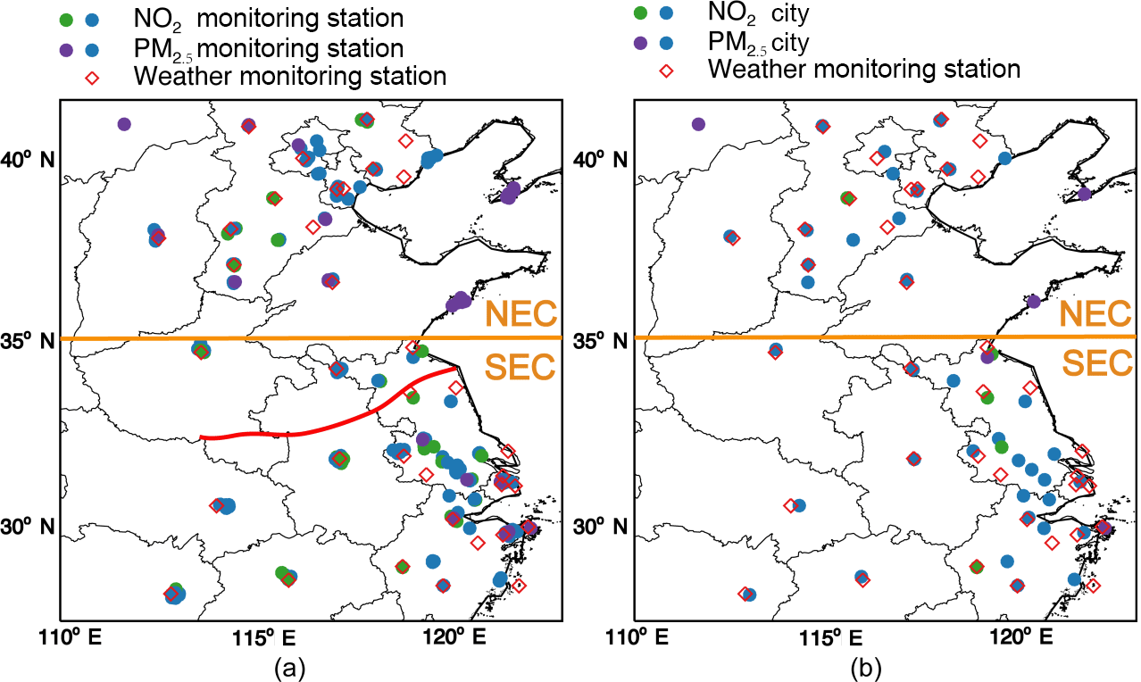
Figure 1(a) Distribution of 163 measurement stations for NO2, 157 stations for PM2.5, and 36 meteorological stations (red diamonds) over Eastern China (25–41∘ N, 110–123∘ E). (b) Distribution of 42 cities with NO2 and PM2.5 observations. Both dots denote stations (a) and cities (b) with both NO2 and PM2.5 data. The blue dots indicates the same stations (cities) for both NO2 and PM2.5, while the green dots are only used for NO2 and purple dots are only used for PM2.5. The orange line separates northern Eastern China (NEC) and southern Eastern China (SEC), and the red line labels the location of the Huai River.
For PM2.5 over China, both the diurnal and the day-to-day variations are complicated by its relatively long lifetime, its various components from different sources, and meteorology. Liu et al. (2016) suggested three types of PM2.5 diurnal cycle within a year, with the peak concentration occurring at distinctive hours in different seasons. In the summertime (April to August), the diurnal cycle may follow human activities (Gong et al., 2007; Liu et al., 2016), which is different from the diurnal cycles in the biomass burning season or in winter. Other studies suggested weak diurnal cycles of PM2.5 in urban or suburban areas (Chen et al., 2015; Hu et al., 2014). Moreover, some studies pointed to the lack of a weekly cycle of PM2.5 (Liu et al., 2016), while others suggested contrasting weekly cycles (for Beijing, Chen et al., 2015; Hu et al., 2014). In winter, the frequent and irregular weather systems prohibit a clear weekly cycle (Gong et al., 2007).
This study analyzes the spatiotemporal variability of NO2 (with the shortest lifetime of hours and the greatest variability among the pollutants measured by the official monitoring network) and PM2.5 (the dominant air pollutant for premature mortality; Forouzanfar et al., 2015) over Eastern China in fall–winter 2013. Given the complex and nonstationary nature of pollutant variability over Eastern China, here we compile an EOF–EEMD analysis visualization package to simultaneously distinguish and visualize the spatial and temporal variability of pollutants. In sequence, the package consists of an empirical orthogonal function (EOF) analysis (Lorenz, 1956) to separate spatial and temporal patterns, an ensemble empirical mode decomposition (EEMD) analysis (Wu et al., 2009) to separate different temporal modes, a Hilbert transform (HT), a marginal spectrum analysis (MSA), and a visualization step to present all physically meaningful spatial and temporal modes in a two-dimensional plot. In particular, EEMD (Huang, 2005; Huang et al., 1998, 1999; Huang and Attoh-Okine, 2005; Wu et al., 2009) is an effective tool to extract signals from noisy nonlinear and nonstationary processes (Wu et al., 2009). EEMD and its variants (e.g., multidimensional ensemble empirical mode, MEEMD) have been widely used in climate studies (Feng et al., 2014; Huang et al., 2012a, b; Vecchio and Carbone, 2010; Wu et al., 2011, 2016). The EOF–EEMD package thus allows for quantitative manifestation of the spatial, (regular) diurnal, and (irregular) day-to-day variations of pollutants and meteorological drivers.
We further use the EOF–EEMD package to evaluate how well chemical transport models (CTMs) can reproduce the observed pollution variability. Although popularly used in air pollution diagnosis, forecast and projection, and remote sensing (Geng et al., 2015; Lin et al., 2015), models are subject to errors in emissions, chemistry, transport, PBL mixing, and other processes (Lin et al., 2008, 2012; Zhang et al., 2016b). This study evaluates two representative models, GEOS-Chem and WRF/CMAQ, with a note that such an evaluation can be applied to other models.
The rest of the paper is organized as follows. Section 2 introduces in situ measurements of NO2, PM2.5, meteorological parameters, model simulations, and the EOF–EEMD analysis visualization package. Section 3 analyzes the observed spatiotemporal variations of NO2 and PM2.5, including their relationships with meteorological parameters. Section 4 evaluates the modeled spatiotemporal variations of NO2 and PM2.5. Section 5 concludes the present study with further discussion on the applicability of the EOF–EEMD package.
2.1 Spatial and temporal domain
We focus on pollution over Eastern China (25–41∘ N, 110–123∘ E). Guided by an EOF analysis, we contrast pollution over the southern (SEC, south of 35∘ N) and northern (NEC) parts to address the regional differences in day-to-day pollution variability. Such latitudinal separation coincides with the Huai River climate transitional zone (Ye and Li, 2017). The orange lines in Fig. 1 separate the two regions.
Our study period is from 25 October to 25 December 2013, with a total of 1488 h in 62 days. Most air pollution data are missing in January and February 2014 because of instrumental failure or data retrieval failure, and data before 25 October are not available.
2.2 NO2 and PM2.5 observations
We retrieve hourly measurements of NO2 and PM2.5 from 193 air quality monitoring stations of the MEP. Most stations are located in urban areas, and only six stations are suburban. As almost every station has missing values in more than one day, we exclude stations that have missing values at ≥30 % of the 1488 h or during a consecutive 72 h period. We thus select 163 stations for NO2 and 159 stations for PM2.5 in the same 42 cities. The dots in Fig. 1a and b depict the stations and cities, respectively. The blue dots show stations and cities with both valid NO2 and PM2.5, the green dots with NO2 only, and the purple dots with PM2.5 only. The slight difference between NO2 and PM2.5 stations does not affect our analysis of the regional pattern of pollutants.
2.2.1 Correction of raw NO2 measurements
At the monitoring sites, NO2 is measured via molybdenum-catalyzed conversion to nitric oxide (NO) and a subsequent chemiluminescence measurement. The measurement technique suffers from interference by more oxidized nitrogen species, since the heated molybdenum surface exhibits low chemical selectivity (Boersma et al., 2009; Lamsal et al., 2008; L. Zhang et al., 2016)
Here we follow Lamsal et al. (2008) to correct for the interference by introducing a correction factor (CF) based on GEOS-Chem-simulated nitrogen species (NO2, HNO3, PAN, and all alkyl nitrates (∑AN)).
We multiply CF with the raw NO2 data to obtain “corrected” NO2 concentrations. Our sensitivity test suggests that assuming PAN and HNO3 to be fully converted to NO2 (i.e., assuming the coefficients to be unity for both PAN and HNO3 in Eq. 1) does not affect our spatiotemporal analysis of NO2. Hereafter the NO2 corrected by Eq. (1) is discussed, unless stated otherwise.
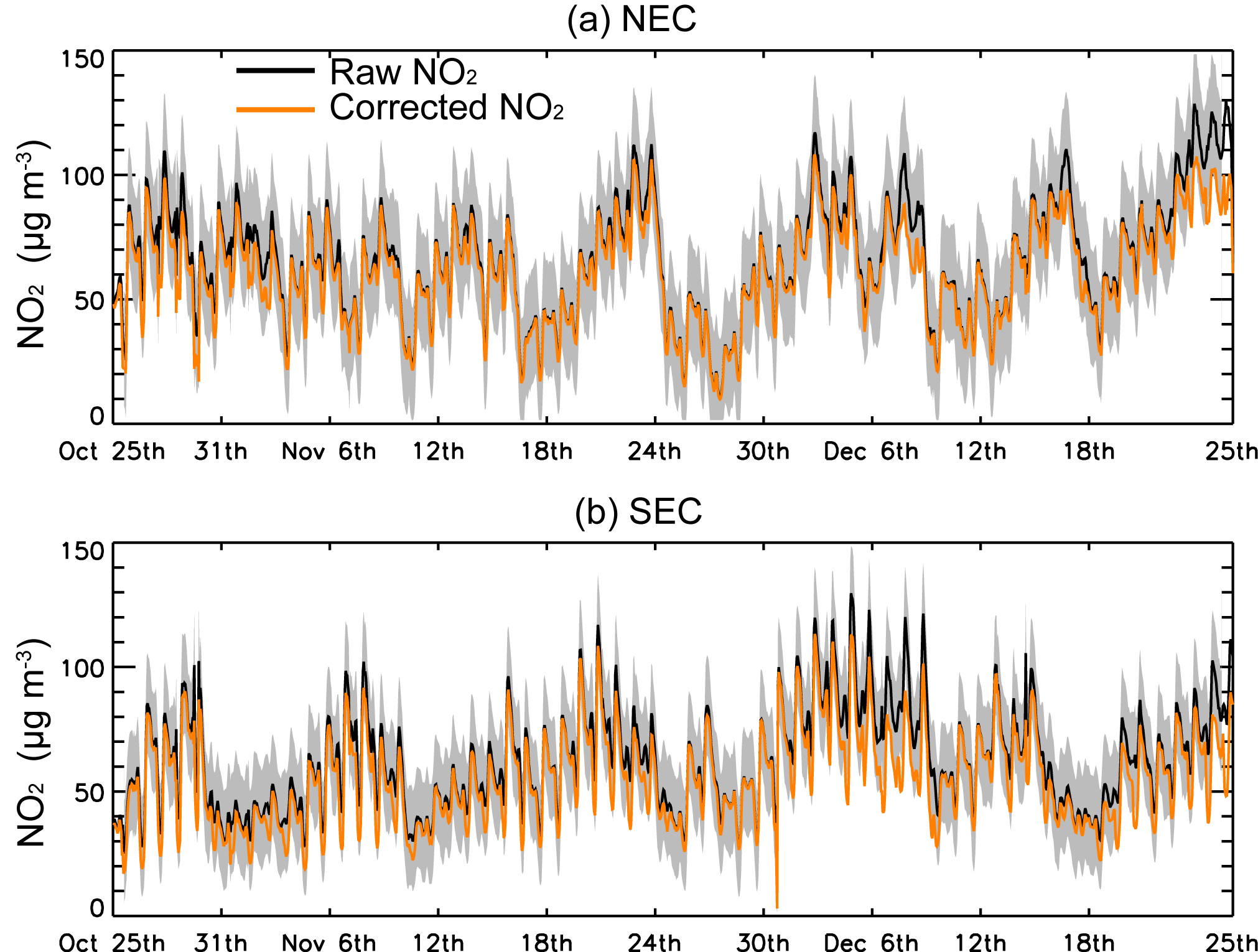
Figure 2Regional mean hourly time series of raw and “corrected” NO2 from the observations. The gray shading indicates 1 standard deviation across all stations.
Figure 2 compares the regional mean hourly time series of raw and corrected NO2. The correction reduces NO2 concentrations by about 2–30 µg m−3 over the whole period and is higher at times when nitrogen is more oxidized. It slightly reduces the relative contribution of day-to-day variability to the total variance of NO2 under the EOF–EEMD analysis (not shown) because excluding the more oxidized species shortens the lifetime of NO2.
2.2.2 Filling in missing values for EOF–EEMD analysis
Prior to an EOF–EEMD analysis, we fill in missing values in hourly pollution observations. If data are missing for more than a consecutive 12 h period, we fill in the missing value in each hour with data on that hour averaged over all days; as such, the diurnal cycle is maintained. In other cases, linear interpolation from adjacent valid data is applied. Our interpolation does not introduce significant artificial information for spatiotemporal analysis, as validated by a sensitivity test with GEOS-Chem model data. Specifically, the EOF–EEMD results based on the original GEOS-Chem data (i.e., no missing values) are similar to the results based on model data sampled at times of valid observations with missing values filled in with the same technique as for the observation data.
2.2.3 Conversion from station- to city-based datasets
Since different cities have different numbers of stations, we calculate city mean observations by averaging across all stations of each city. Compared to a station-based analysis, the city-based EOF–EEMD results reduce the spatial noise, leading to more distinctive temporal patterns. All analyses hereafter are based on city mean data. The longitude and latitude of each city center are used to identify the respective model grid cell.
2.3 Meteorological observations
We use 3-hourly measurements of 2 m air temperature, 2 m relative humidity, and 10 m wind speed from meteorological stations recorded at the National Oceanic and Atmospheric Administration National Centers for Environment Information (NOAA NCEI). We do not use surface pressure additionally because it is highly correlated with air temperature and relative humidity on the day-to-day scale. The locations of these stations do not always coincide with air pollution stations. Thus, we select 36 meteorological stations within 10 km of air pollution stations (red hollow dots in Fig. 1). Despite the difference (in number and location) between pollution and meteorological stations, an analysis of the regional temporal patterns of pollutants and meteorology is still informative (see Sect. 3.2).
To fill in missing values, we apply an interpolation process that accounts for diurnal variability using information for an adjacent day. For example, if the temperature on 26 October at 12:00 is missing, we calculate the temperature difference between 09:00 and 12:00 on the 25th as well as the difference between 15:00 and 12:00 on the 25th. We then use these differences to adjust the temperatures at 09:00 and 15:00 on the 26th, and finally use the mean of the two adjusted temperatures as the temperature on the 26th at 12:00.
For consistency with the hourly pollution data, we linearly interpolate the 3-hourly meteorological measurements to each hour. This interpolation does not distort the EOF–EEMD analysis, as confirmed by comparing the statistical analysis on 1-hourly GEOS-FP meteorological parameters versus an analysis on 3-hourly GEOS-FP data. Note that the GEOS-FP meteorology is used to drive GEOS-Chem.
2.4 Model simulations
2.5 GEOS-Chem
We use the nested GEOS-Chem CTM version 9-02 (L. Zhang et al., 2016) to simulate NO2, PM2.5, and other pollutants over China in October–December 2013. The model resolution is a 0.3125∘ long. × 0.25∘ lat. grid with 47 vertical layers, and the lowest 10 layers are of ∼130 m thickness each. The model is driven by the GEOS-FP assimilated meteorology from the National Aeronautics and Space Administration (NASA) Global Modeling and Assimilation Office, with the full Ox–NOx–VOC–CO–HOx gaseous chemistry (Mao et al., 2013) and online aerosol calculations. Vertical mixing in the PBL adopts a nonlocal scheme (Holtslag and Boville, 1993; Lin et al., 2010). Model convection is simulated with the relaxed Arakawa–Schubert scheme (Rienecker et al., 2008).
Chinese anthropogenic emissions of NOx and other pollutants adopt the monthly MEIC inventory with a base year of 2010 (http://www.meicmodel.org, last access: 1 December 2015) (Geng et al., 2017). We further use the monthly DOMINO v2 NO2 data to scale monthly anthropogenic NOx emissions from 2010 to the simulation year (Lin et al., 2015). The emission scaling improves the simulation of NO2 (Cui et al., 2016). Other model setups are referred to Lin et al. (2015) and Yan et al. (2016).
GEOS-Chem modeled PM2.5 includes secondary inorganic aerosols (sulfate, nitrate, and ammonium), black carbon, primary organic carbon, natural dust, and sea salt. Secondary organic aerosols are not included in this study, considering the severe underestimate in China due to missing precursor emissions and formation pathways (Fu et al., 2012; L. Zhang et al., 2016). Anthropogenic dust is also not included.
The nested model simulation is from 15 October to 25 December in 2013, allowing for a 10-day spin-up period. Its lateral boundary conditions of chemicals are updated every 3 h by results from a corresponding global simulation on a 2.5∘ long. × 2∘ lat. grid. Modeled NO2 and PM2.5 in the first layer are sampled at city centers and times with valid observations, unless stated otherwise.
2.5.1 CMAQ
We use the Weather Research and Forecasting (WRF) model v3.5.1 (http://www.wrf-model.org/, last access: 1 December 2015) to drive CMAQ v5.0.1 (http://www.cmascenter.org/cmaq/, last access: 1 December 2015). The simulation covers East Asia at a horizontal resolution of 36×36 km2 with 14 vertical layers. The lowest six layers are of ∼80 m thickness each, and about eight layers are below 1 km. The gas-phase chemistry uses the CB05 mechanism with active chlorine chemistry and updated toluene mechanism (Whitten et al., 2010). The aqueous-phase chemistry adopts the updated Regional Acid Deposition Model (RADM) (Chang et al., 1987; Walcek and Taylor, 1986). The aerosol chemistry follows AERO6. PBL mixing in both WRF and CMAQ adopts the ACM2 scheme (Pleim, 2007). Other model physics are detailed in Zheng et al. (2015).
Chinese anthropogenic emissions are from MEIC (http://www.meicmodel.org, last access: 1 December 2015). Emissions in 2013 are extrapolated from the base year (2012) based on country-level statistics (Zheng et al., 2015). Anthropogenic emissions in other Asian countries and biomass burning emissions are taken from the MIX emission inventory prepared for the Model Inter-Comparison Study Asia Phase III (MICS-ASIA III).
The PM2.5 species in AERO6 include fine-mode sulfate, nitrate, ammonium, primary and secondary organic aerosols, black carbon, sodium, calcium, aluminum, particulate chloride, and the remaining unspeciated fine-mode primary PM (http://www.airqualitymodeling.org/cmaqwiki/index.php?title=CMAQv5.0_PMother_speciation, last access: 30 November 2017).
The simulation is from 15 October to 25 December 2013, allowing for a 10-day spin-up period. Initial conditions and boundary conditions are from GEOS-Chem (Zheng et al., 2015). Modeled NO2 and PM2.5 in the first layer are sampled at city centers and times with valid observations, unless stated otherwise.
2.6 EOF–EEMD analysis visualization package
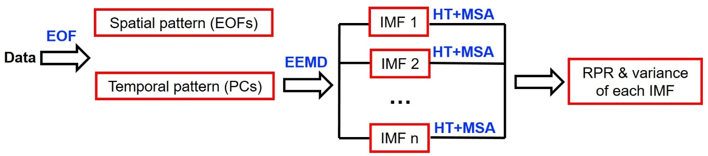
Figure 3The flowchart of the EOF–EEMD analysis visualization package. The red boxes represent the quantities visualized.
As shown in Fig. 3, our EOF–EEMD analysis visualization package consists, in order, of an EOF analysis (Lorenz, 1956), an EEMD analysis (Wu et al., 2009), a Hilbert transform (HT) with marginal spectrum analysis (MSA), and a visualization step to quantitatively depict the spatial–temporal scales of measurement or model data.
The basic purpose of our package is to quickly and simultaneously identify and visualize various spatial and temporal scales of interest in the observation or model datasets. As shown by Feng et al. (2014) and Wu et al. (2016), combining EOF with EEMD to decompose the datasets leads to a faster calculation than MEEMD by 1 or 2 orders of magnitude because here the EEMD is applied to the temporal components (i.e., PCs) out of an EOF analysis rather than to all dimensions. Also, our EOF–EEMD package conducts additional HT–MSA and provides visualization of all spatial and temporal scales of interest.
-
EOF analysis to decompose a two-dimensional dataset (time series at multiple locations) into spatial and temporal components.
Suppose there are n locations, each having a time series of length p. The associated dataset Z is an n×p matrix. An EOF analysis of Z gives
Here Σ is a diagonal q×q matrix containing the first q singular values of Z, and it represents the contribution of each pattern to the total variance of Z. The diagonal values of Σ are in a descending order, and thus the first several modes are the dominant ones. U is an n×q matrix representing the spatial component, and each column of U represents a spatial mode. W is a p×q matrix representing the temporal component, and each column of W represents a principal component (PC) for temporal variation associated with the corresponding spatial mode.
-
EEMD analysis of each PC time series to obtain its “intrinsic mode functions” (IMFs) of descending frequencies.
Each PC is mixed with multiple scales, which requires further decomposition in the time domain. Unlike fast Fourier transform (FFT) or wavelet transform (WT), EEMD does not need a priori bases, and it can be appropriately applied to delineate nonlinear and nonstationary time series, as in our pollution study.
EEMD consists of an ensemble of empirical mode decomposition (EMD) performed on each PC time series (denoted as x(t) in Eq. 3). Each EMD linearly decomposes x(t) into individual IMFs cj (of ascending timescales and descending frequencies) and a residual rn:
EMD is based on finding the local maxima and minima of the time series. A detailed decomposition process can be found in Huang et al. (1998, 1999). EMD is much less susceptible to missing values and data interpolation than approaches that are based on an analysis of the whole time series (e.g., FFT and WT).
EMD may be sensitive to noise in the real data to encounter a “mode mixing” problem (Wu et al., 2009). EEMD solves this problem by performing an ensemble of hundreds of EMDs, each with certain white noise added to x(t). Hence, the noise in the real data is incorporated as part of the white noise, and the ensemble further minimizes the effects of noise. The white noise is assumed to follow the standard Gaussian distribution (Wu et al., 2009). Figure 4 shows an example of the EEMD analysis.
-
Hilbert transform and marginal spectrum analysis of each IMF to reveal its representative frequency range.
There are no discrete periods or frequencies in the pollution and meteorological time series. Correspondingly, an IMF also has a continuous frequency range (rather than a constant frequency) that can be determined by HT–MSA. The HT reveals the IMF energy–frequency–time distribution (Huang et al., 1999). The MSA further shows the IMF distribution of variance (energy) with respect to different frequencies. The spectral peak represents the largest contribution to total variance.
A spurious oscillation may occur near the edges of certain IMF time series, resulting in an inaccurate calculation of variance under HT–MSA. We apply a box-car filter (Gubbins, 2004) to select the internal 60 % of an IMF time series (from 20 % to 80 % of the 1488 h) to perform HT–MSA. Figure 4b shows an example of the visualized result of HT–MSA, in which the horizontal axis is the number of occurrences within the whole period (frequency, in h−1, multiplied by the time length, 1488 h) and the vertical axis is the energy contribution. IMF2–IMF5 are visualized and analyzed in this study. The higher-frequency IMF1 is noisy as the energy is distributed over a wide range of occurrence numbers. IMF6–IMF10 represent the longest temporal scales that contribute little to the total variance of the decomposed PC. Thus IMF1 and IMF5–IMF10 are not further analyzed.
Based on HT–MSA, we determine a representative frequency range (RFR) such that the range encompasses the peak frequency and that the frequencies within the range contribute 50 % of the total variance of an IMF. The frequencies below and above the RFR bounds each contribute 25 % of the total variance of the IMF. Before calculating the RFR, we smooth the marginal spectrum by connecting all local maxima of the spectrum with a cubic spline.
-
Visualization of the spatial and temporal scales in a two-dimensional plot.
Finally, we simultaneously visualize the spatial and temporal scales as well as their contributions to the total variance of Z in a two-dimensional plot for easy observational diagnosis and model evaluation. In this plot, an IMF is represented by a vertical “error bar” and a horizontal bar. The length of the error bar stands for the representative period range (RPR, the inverse of RFR), and a shorter length means a more stationary variation mode (i.e., towards a fixed frequency or period). The length of the horizontal bar stands for the contribution to the total variance. For clearer presentation, the plot does not include IMFs that do not pass the white noise examination, that lay outside the range of scales considered here (hours to days), or that contribute little to the total variance of the original data (e.g., less than 1 %).
3.1 General characteristics

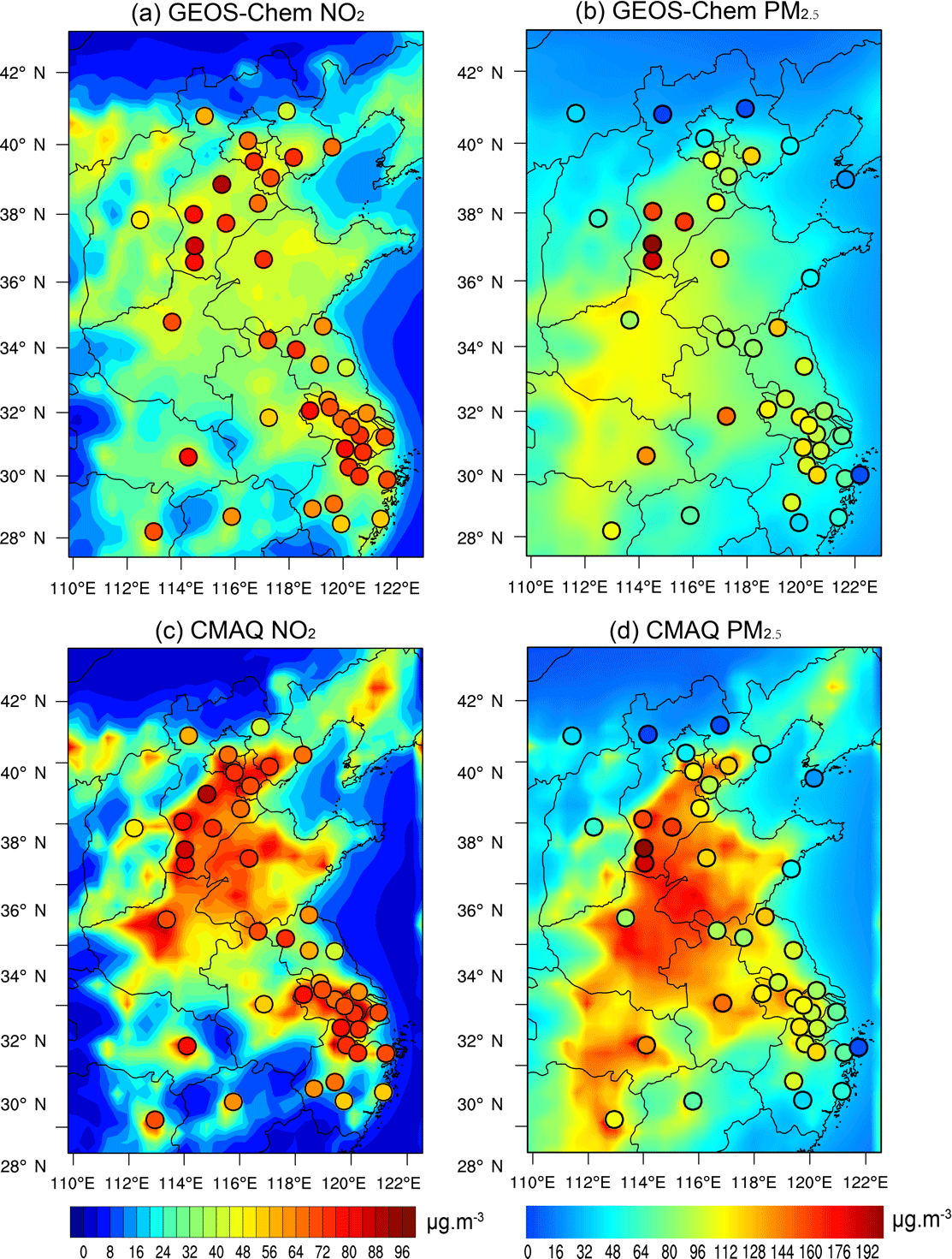
Figure 5Observed (filled circles) and modeled (color maps) NO2 and PM2.5 averaged over 25 October–25 December 2013. Here the model results are averaged over all days rather than sampled at times of valid observations.
The colored dots in Fig. 5a and b show the observed spatial distributions of city mean NO2 and PM2.5 averaged over the time period. Both NO2 and PM2.5 are largest over Beijing–Tianjin–Hebei (BTH) in the north and the Yangtze River Delta (YRD) in the east. NO2 concentrations exceed 60 µg m−3 at many sites. The range of PM2.5 is larger, from below 10 µg m−3 in some northern and coastal cities to about 200 µg m−3 in several cities of BTH.
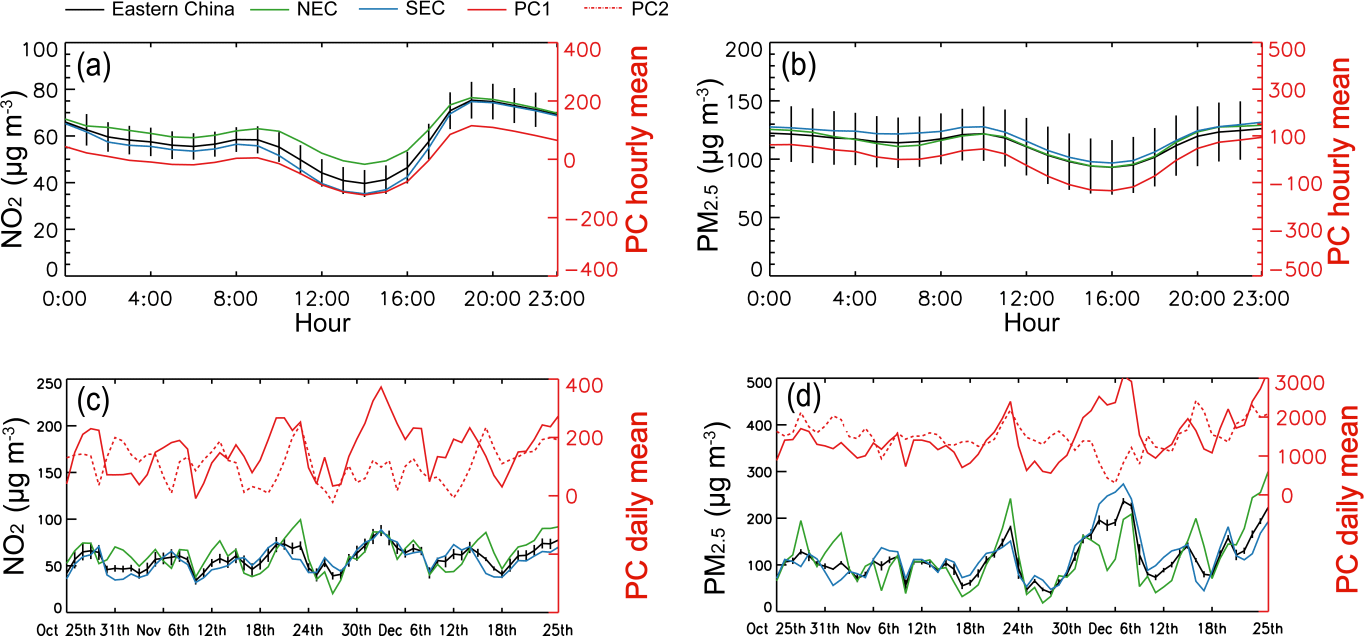
Figure 6(a) Diurnal variation of observed NO2 averaged over 25 October–25 December 2013. The black vertical bars represent 1 standard deviation across the days. PC1 from the EOF analysis is overlaid in red. (b) Similar to (a) but for PM2.5. (c) Day-to-day variation of daily mean NO2 over 25 October–25 December 2013. Data are de-trended. The black vertical bars represent 1 standard deviation due to the diurnal variation. PC1 and PC2 from the EOF analysis are overlaid in red. (d) Similar to (c) but for PM2.5.
Figure 6a and b show the diurnal variations of NO2 and PM2.5 over Eastern China, NEC, and SEC averaged over all days. Similarly, over the three regions, NO2 peaks around 19:00 due to evening rush hour emissions, reduced PBL mixing, and a lengthened lifetime. NO2 reaches a minimum at 14:00 because of the shortest lifetime and strongest PBL mixing. The diurnal range (maximum minus minimum) is about 30 µg m−3. The PM2.5 level also reaches a minimum in the early afternoon. It has a much smaller diurnal range at 10 µg m−3. The vertical error bars in Fig. 6a and b depict the standard deviation for the day-to-day variation of NO2 and PM2.5 at any given hour. At a given hour, the PM2.5 level is much more variable across the days than NO2. In particular, the day-to-day standard deviation for PM2.5 at a given hour is as large as the diurnal range of PM2.5.
Figure 6c and d further show the time series of daily mean NO2 and PM2.5. All data are de-trended (trends are at 0.01 µg m−3 h−1 for NO2 and 0.05 µg m−3 h−1 for PM2.5). Although local maxima and minima (peaks and troughs of the time series) occur every several days, there is no single period or amplitude for the variation of each species. For NO2 over Eastern China (black line in Fig. 6c), the local maxima vary from 60 to 100 µg m−3, and the local minima vary from 20 to 40 µg m−3. For PM2.5 over Eastern China (black line in Fig. 6d), the local maxima vary from 100 to 300 µg m−3, and the local minima vary from 20 to 120 µg m−3. Furthermore, comparing the green and blue lines reveals that pollutants over NEC and SEC synchronize on some days but are out of phase on others; this feature is quantitatively analyzed in Sect. 3.2. These day-to-day variation patterns are associated with meteorological conditions and pollutant lifetimes.
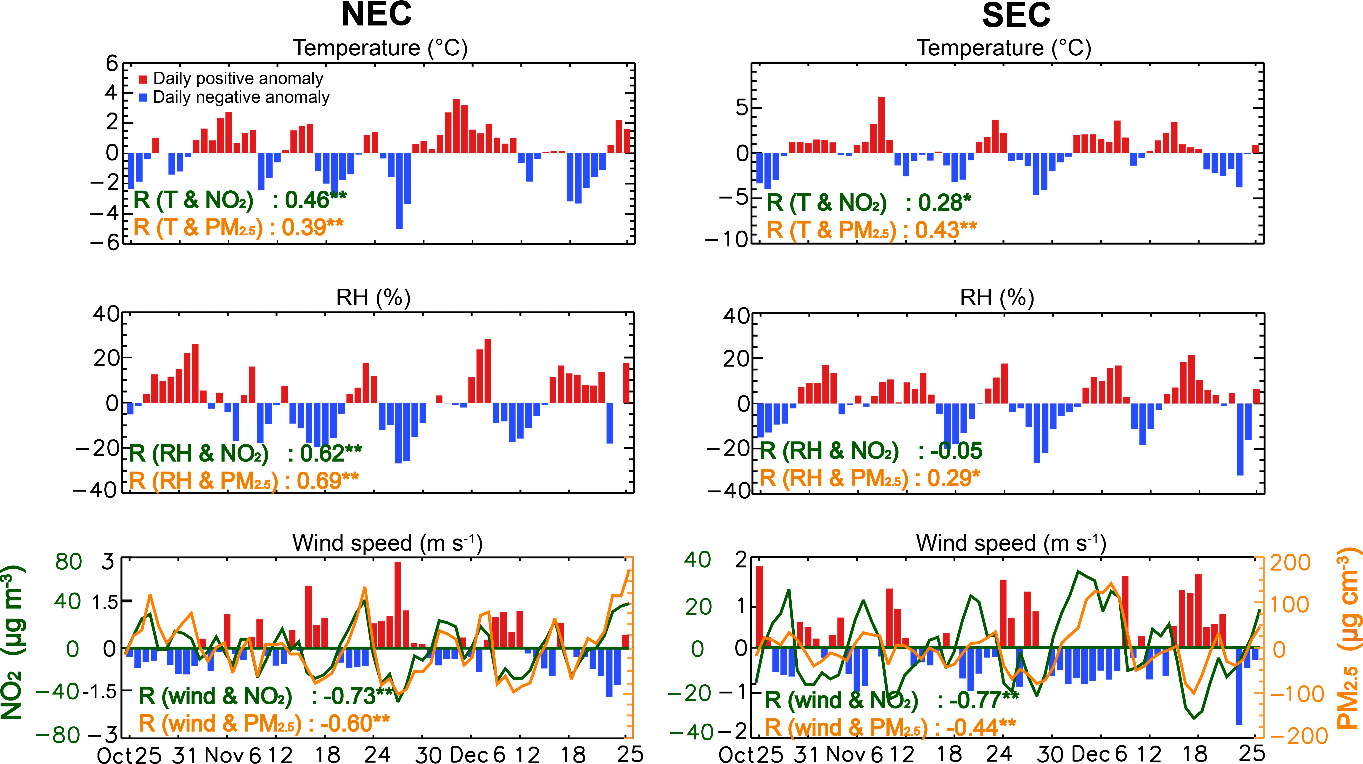
Figure 7Daily anomalies of observed meteorological parameters and pollutant concentrations averaged over NEC and SEC, as well as their correlations. All data are de-trended. Correlation coefficients with “*” and “**” are statistically significant with P values below 0.05 and 0.01, respectively.
Figure 7 shows day-to-day anomalies of observed pollutant concentrations and meteorological parameters over NEC and SEC. All data are de-trended. Over NEC, wind speed is clearly anticorrelated with pollutant levels. The correlation coefficient reaches −0.73 between NO2 and wind speed and −0.60 between PM2.5 and wind speed. Over this region, stronger winds are often associated with lower RH and lower temperature, characteristic of a cold air passage that brings cleaner, colder, and drier air from the north to NEC and transports the NEC pollution out of the region. Correspondingly, RH is strongly positively correlated with NO2 (R=0.62) and PM2.5 (R=0.69). The meteorology-associated day-to-day variability is more apparent after mid-November, when the variations of the two pollutants are more synchronous.
Over SEC (Fig. 7), the relationship between pollutant levels and meteorological parameters is more complex. The correlation between daily mean PM2.5 and wind speed is relatively weak ( compared to −0.60 over NEC), and its correlation with RH is even weaker (R=0.29). This indicates that the northerly air does not reduce PM2.5 levels over SEC as effectively as over NEC, as PM2.5 from NEC may be transported to SEC. By comparison, NO2 is still highly anticorrelated with wind speed () over SEC, likely a result of the short lifetime of NO2. Compared to PM2.5 whose lifetime is sufficiently long (several days) for transport from NEC to SEC (Hu et al., 2014), NO2 has a much shorter lifetime (below 1 day; Lin et al., 2012) and cannot undergo effective long-distance transport. However, almost all pollution measurement sites are urban, and weaker (stronger) winds allow for rapid accumulation (removal) of urban NO2 pollution.
3.2 EOF–EEMD analyses of pollutants and meteorological parameters
Although informative, the time series analyses of regional mean pollution in Sect. 3.1 do not provide adequate quantitative information on the spatiotemporal variability and embedded scales. In fact, the separate discussion on NEC and SEC in Sect. 3.1 is largely inspired by the following EOF–EEMD analysis that suggests distinctive features between these two subregions. In this section, we use the EOF–EEMD package to distinguish and visualize the quantitative contributions of individual spatial and temporal modes to variations in the pollutant and meteorological data.
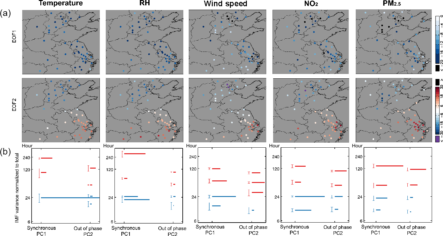
Figure 8EOF–EEMD–HT–MSA results for the observed temperature, RH, wind speed, NO2, and PM2.5. The first two rows depict EOF1 and EOF2, and the third row shows the EEMD–HT–MSA result for PC1 and PC2. In each panel of the third row, the length of the vertical “error bar” shows the RPR of an IMF, while the length of the horizontal bar represents the percentage contribution of the IMF to the total variance of the original data (as such, the horizontal lengths for different IMFs across different PCs can be compared). The blue (red) color indicates diurnal (day-to-day) variation.
The columns in Fig. 8 show the EOF–EEMD results for the observed temperature, RH, wind speed, NO2, and PM2.5. The first two rows show the first two spatial patterns (EOF1 and EOF2) from the EOF analysis. The third row visualizes the EEMD–HT–MSA results for PC1 and PC2, the temporal counterparts of EOF1 and EOF2. For all variables, the first two PCs contribute more than 50 % of the total variance of the original data. The following PCs (PC3, PC4…) contain small variances and are not discussed here.
3.2.1 EOF–EEMD analyses of pollutants
The fourth column in Fig. 8 for NO2 shows a primary pattern (EOF1 and PC1) with synchronous variation over the entirety of Eastern China. This pattern contributes 42 % of the total variance of NO2. The two dominant IMFs of PC1 have time periods at 24 and 12 h, respectively, and together they contribute 30.4 % of the total variance of NO2. Thus, PC1 mainly reflects the diurnal variation of NO2. PC1 also contains some day-to-day variability in IMFs, which contribute about 10 % of the total variance of NO2. The second pattern (EOF2) of NO2 reveals opposite temporal variations between NEC and SEC. This temporal contrast is mainly reflected in the day-to-day variability, with RPRs around 2–5 days contributing 10.9 % of the total variance in NO2. The day-to-day components of PC1 and PC2 correspond to the finding in Sect. 3.1 that NO2 over NEC and SEC is synchronous on some days but out of phase on others.
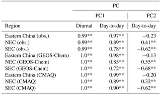
We further investigate the physical meanings of PC1 and PC2 for NO2. The red solid and red dashed lines in Fig. 6a and c show the diurnal and day-to-day variations of PC1 and PC2 in comparison to regional mean NO2 levels over Eastern China (black line), NEC (green line), and SEC (blue line). Table 1 shows the associated correlation coefficients. PC1 is synchronous with Eastern China mean NO2 for both diurnal and day-to-day variations (R reaches 1.0), confirming this regionally synchronous pattern. The day-to-day variation of PC2 is correlated with NEC NO2 (R=0.66) but anticorrelated with SEC NO2 (, Table 1), again confirming this NEC–SEC contrasting pattern.
Table 1Correlation between PCs and regional mean values in terms of diurnal and day-to-day variability for NO2.
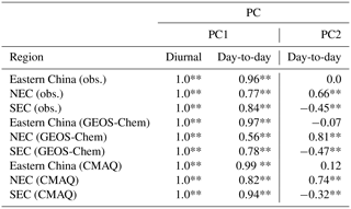
** The correlation coefficient is statistically significant with the P value <0.01.
The last column in Fig. 8 shows the EOF–EEMD result for PM2.5. As for NO2, EOF1 and PC1 of PM2.5 reflect a temporally synchronous pattern over Eastern China, which contributes 44 % of the total variation of PM2.5. Again, PC1 is synchronous with Eastern China mean PM2.5 (red versus black lines in Fig. 6b, d) in terms of both diurnal and day-to-day variations, with correlation coefficients approaching 1.0 (Table 2). However, the IMFs of PC1 representing diurnal variation are relatively weak, consistent with the noisy diurnal cycle of PM2.5 discussed in Sect. 3.1. The dominant IMF of PC1 shows a period of around 7 days. PC2 of PM2.5 reflects the day-to-day contrast between NEC and SEC (Fig. 6d and Table 2) with RPRs of 2–5 days, similar to PC2 of NO2.
Table 2Correlation between PCs and regional mean values in terms of diurnal and day-to-day variability for PM2.5.
** The correlation coefficient is statistically significant with the P value <0.01.
3.2.2 EOF–EEMD analyses of meteorological parameters
For comparison, the first three columns in Fig. 8 show the EOF–EEMD results for the observed temperature, RH, and wind speed. The EOF–EEMD result for wind speed (the third column in Fig. 8) is closest to that for NO2, with a regionally synchronous pattern (EOF1 and PC1), an NEC–SEC contrasting pattern (EOF2 and PC2), and a dominant IMF with a period of 24 h. The day-to-day wind speed variability is also reflected in the IMFs of PC1 and PC2 with RPRs of 2–5 days, consistent with that for NO2. The EOF–EEMD result for wind speed is also fairly comparable with that for PM2.5, although the latter shows a dominant IMF (in PC1) with a period of 7 days. These results are consistent with Sect. 3.1 but with a more quantitative analysis on the spatiotemporal scales.
The EOF–EEMD analysis for temperature (the first column in Fig. 8) shows that PC1 contributes 88 % of the total variance, and it is dominated by the IMF with a period of 24 h. The contribution of PC2 is negligible (4 %). For RH (the second column in Fig. 8), PC2 plays a minor role, and there are IMFs of PC1 with periods near 3 and 12 days, contributing to the correlation between RH and PM2.5. These results indicate a complex association in the day-to-day variability between temperature–RH and pollutants broadly consistent with the discussion in Sect. 3.1.
4.1 General evaluation
The color contours in Fig. 5a–d show the horizontal distributions of NO2 and PM2.5 simulated by GEOS-Chem and CMAQ. The model results here are averaged from all days over the time period rather than sampled from days with valid observations. Both models capture the general spatial patterns of observed NO2 and PM2.5, with the heaviest pollution over the north and east.
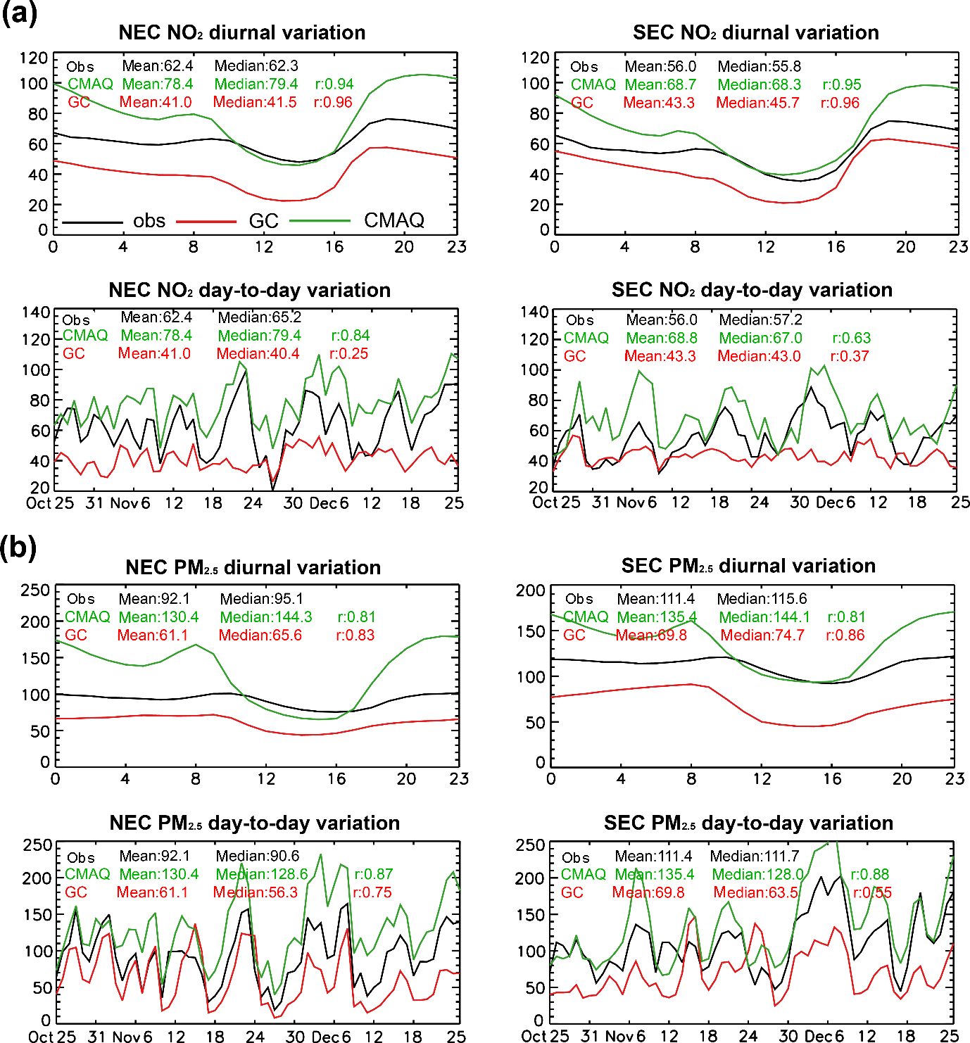
Figure 9Observed and simulated diurnal and day-to-day variations of (a) NO2 and (b) PM2.5 over NEC and SEC (µg m−3).
Figure 9 evaluates the regional mean diurnal and day-to-day variations of modeled pollutant levels over NEC and SEC. Here model data are sampled from days and locations with valid observations. All trends are negligible and have been removed, consistent with the observational analysis. GEOS-Chem underestimates the observations by about 17 µg m−3 (21 µg m−3 over NEC and 13 µg m−3over SEC) for NO2 and by 35 µg m−3 over Eastern China (31 µg m−3 over NEC and 41 µg m−3 over SEC) for PM2.5 averaged over the whole period. The model bias is relatively consistent across individual hours. GEOS-Chem captures the observed diurnal variability for both pollutants as well as the day-to-day variability of PM2.5, although it greatly underestimates the day-to-day variability of NO2. More model evaluation statistics are shown in Table 3.
Table 3Observed and simulated pollutants and their correlations.
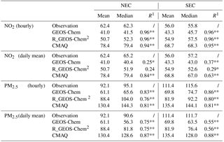
1 Correlation between observed and simulated variables. ** indicates the correlation coefficient is statistically significant with the P value <0.01, while * indicates it passed a statistical test with the P value <0.01. 2 Revised GEOS-Chem NO2 and PM2.5 by multiplying the ratio of the first layer to the second layer of CMAQ values.
Figure 9 also shows that WRF/CMAQ overestimates the nighttime observations by about 30 µg m−3 for NO2 and 60 µg m−3 for PM2.5 averaged over Eastern China, although it reproduces the daytime pollutant levels. This means an overestimate of the diurnal range, as is also revealed by the EOF–EEMD analysis in Sect. 4.2. CMAQ captures the day-to-day variability of daily mean NO2 and PM2.5 much better than GEOS-Chem (R=0.63–0.84 versus 0.25–0.37 over NEC and SEC for NO2; and 0.87–0.88 versus 0.55–0.75 for PM2.5). Note that the correlations shown here mainly reflect the model capabilities to capture Eastern China synchronous day-to-day variation, and they do not imply the model performance in simulating the NEC–SEC contrast, which is revealed in Sect. 4.2. More model evaluation statistics are shown in Table 3.
4.2 Model evaluation based on the EOF–EEMD analysis
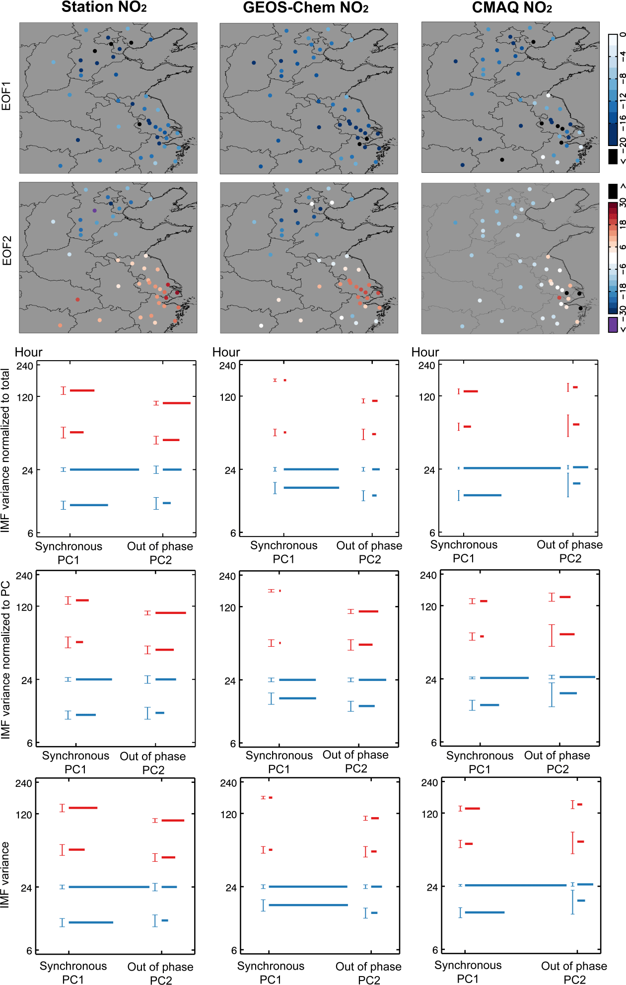
Figure 10EOF–EEMD–HT–MSA results for observed, GEOS-Chem, and CMAQ NO2. See Sect. 4.2 for detailed descriptions.
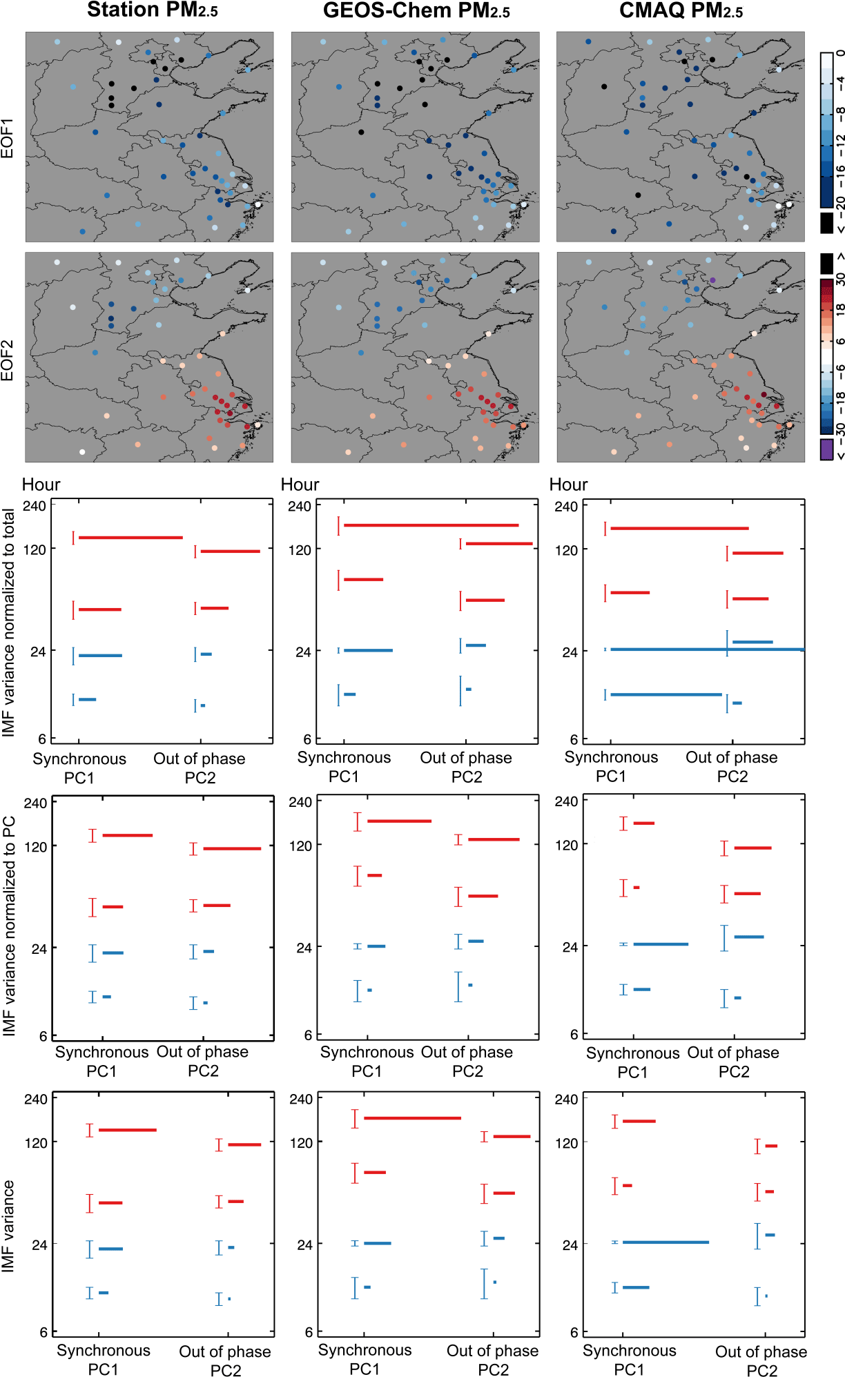
Figure 11EOF–EEMD results for observed, GEOS-Chem, and CMAQ PM2.5. See Sect. 4.2 for detailed descriptions.
Figures 10 and 11 evaluate the EOF–EEMD results for modeled NO2 and PM2.5, respectively. Prior to the EOF–EEMD analysis, modeled NO2 and PM2.5 were sampled at times and locations with valid observations and then underwent the same interpolation procedure to fill in the missing values. In these figures, the last three rows visualize the EOF–EEMD–HT–MSA results in different ways (manifested in different lengths of the horizontal bar for each IMF). In the third row, the variance of each IMF is normalized to the total variance of the original data (NO2 or PM2.5). In the fourth row, the variance of each IMF is normalized to the variance of its respective PC in order to better visualize the signals from PC2 (which has a much smaller variance than PC1); as such, only the IMFs from the same PC are intercomparable. The fifth row visualizes the absolute variance of each IMF without any normalization.
The first two rows in Fig. 10 show EOF1 and EOF2 of NO2. Both GEOS-Chem and CMAQ exhibit a synchronous pattern (EOF1) and an NEC–SEC contrasting pattern (EOF2), consistent with the observation. However, the CMAQ-simulated NEC–SEC contrast in EOF2 is much weaker than the observed. Table 1 shows that for modeled NO2, PC1 is highly correlated with Eastern China mean NO2 for diurnal (R=1.0 for GEOS-Chem and CMAQ) and day-to-day (R=0.56–0.97) variability and that PC2 is correlated with NEC NO2 (R=0.74–0.81) and anticorrelated with SEC NO2 ( to −0.32) in terms of day-to-day variability, in line with the observational analysis.
The last three rows in Fig. 10 show that both models underestimate the contribution of day-to-day variability to the total variance of NO2 (with a shorter length of horizontal bar). For PC1, CMAQ captures the RPR (position of “error bar”) and variance (length of horizontal bar) of the observed IMFs fairly well. By comparison, GEOS-Chem underestimates the day-to-day variance (too-small horizontal length) and does not capture its RPR. These results are consistent with the analysis in Sect. 4.1 (Fig. 9) showing that CMAQ is correlated with the observed Eastern China synchronous NO2 time series much better than GEOS-Chem. For PC2, which reflects the NEC–SEC contrasting pattern, GEOS-Chem outperforms CMAQ in capturing the RPR and variance of the observed day-to-day IMFs (red colored in fourth row). This model characteristic is not seen from the time series discussion in Sect. 4.1.
Figure 11 shows that both GEOS-Chem and CMAQ capture the synchronous pattern (EOF1) and the NEC–SEC contrasting pattern (EOF2) of PM2.5. For PC1, GEOS-Chem captures the variance of each IMF but not its RPR (especially for the day-to-day IMFs). CMAQ simulates too-strong diurnal IMFs, consistent with its overestimated diurnal cycle discussed in Sect. 4.1. CMAQ outperforms GEOS-Chem in capturing the RPR of day-to-day IMFs of PC1, in line with its better correlation with the observations (Fig. 9). For PC2, GEOS-Chem captures the variance and RPR of the observed day-to-day IMFs better than CMAQ.
4.3 Discussion on model deficiencies
WRF/CMAQ overestimates the diurnal variation of NO2 and PM2.5. The causes are multifaceted. The ACM2 PBL mixing scheme in WRF v3.5.1 and CMAQ v5.0.1 (used here) assumes the same value for the eddy diffusivity of momentum (Km) and heat (Kh), which implies a Prandtl number () of unity and too-weak mixing under stable atmospheric conditions (i.e., at night). This deficiency has been alleviated in WRF v3.7 and CMAQ v5.1. Also, there is inconsistency between CMAQ and WRF in the Monin–Obukhov length in the surface layer module. This error has been corrected in CMAQ v5.1. For more model update details, please refer to the online document (https://www.airqualitymodeling.org/index.php/CMAQ_version_5.1_(November_2015_release)_Technical_Documentation, last access: 3 September 2018).
GEOS-Chem (the first model layer) underestimates surface NO2 by about 17 µg m−3 and PM2.5 by 35 µg m−3 averaged over Eastern China. The underestimate of PM2.5 is in part because this simulation of GEOS-Chem does not include secondary organic aerosols, which likely contribute as much as 21 % of PM2.5 over Eastern China (Fu et al., 2012). Also, the model does not include anthropogenic dust. Furthermore, although the observation stations are close to the ground, the first layer of GEOS-Chem is too thick (130 m) to fully capture the vertical gradient of pollution concentrations. Figure 12 shows Eastern China mean vertical profiles of NO2 in the two models. The center of the first layer of CMAQ (40 m) is closer to the ground, and the center of its second layer is located at a height similar to the center of the first layer of GEOS-Chem. CMAQ shows a strong vertical gradient of NO2 from its first to second layer. Had we used the CMAQ-simulated ratio of the first over the second layer to extrapolate GEOS-Chem first-layer NO2 to 40 m, this would significantly increase the model's “ground-level” NO2 (by 24 % over NEC and 17 % over SEC) and PM2.5 (by 45 % and 17 %). However, the extrapolation does not improve the day-to-day correlation to the observations, indicating the important roles played by other factors. See Table 3 for more evaluation statistics.
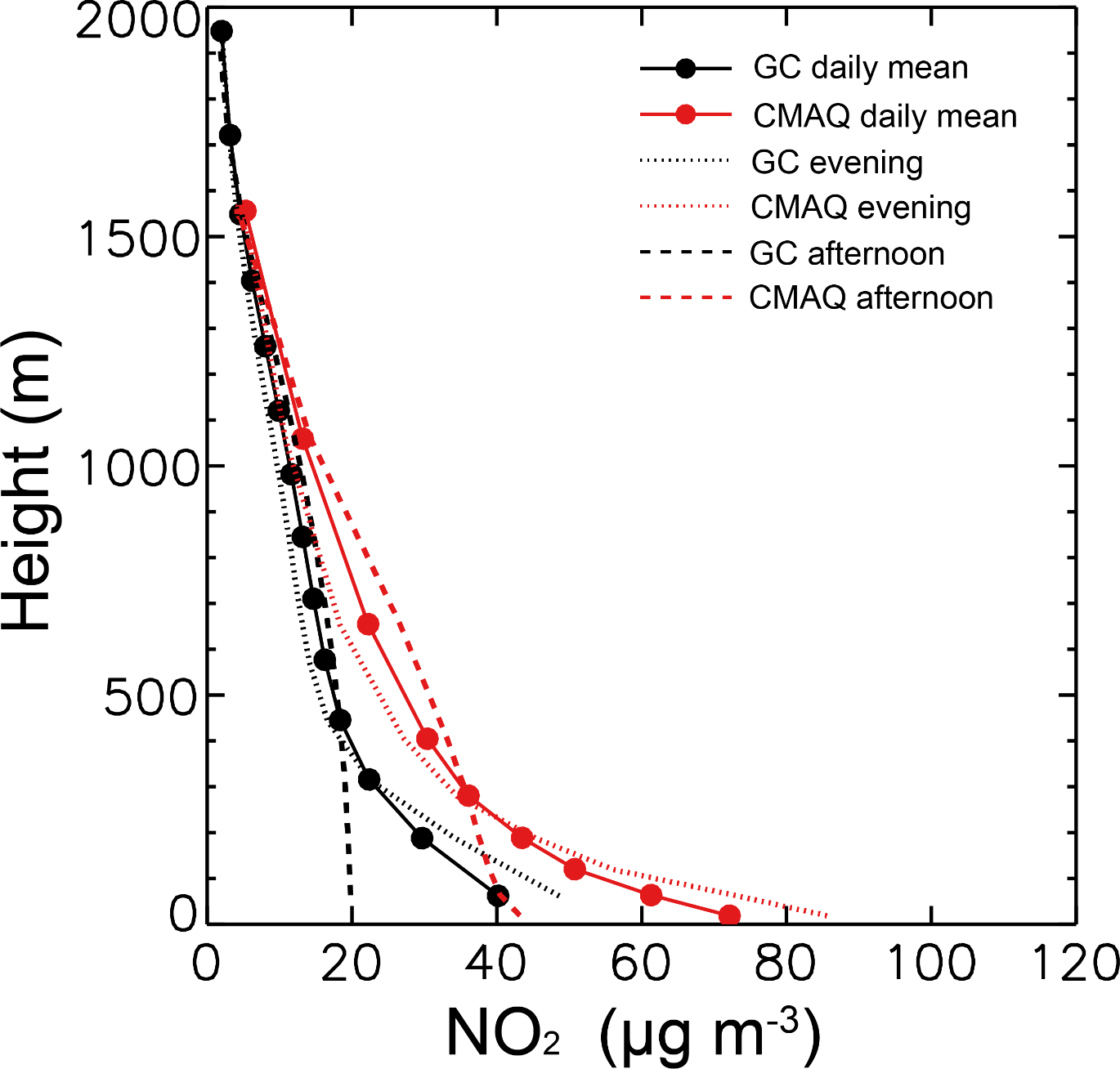
Figure 12Eastern China mean NO2 vertical profiles simulated by GEOS-Chem and CMAQ averaged over 25 October–25 December 2013. The black and red dots denote the center of each vertical layer in the two models. The evening is from 20:00 to 23:00 LT, while the afternoon is from 12:00 to 15:00 LT.
GEOS-Chem (the first model layer) also underestimates the Eastern China synchronous day-to-day variation of NO2. When averaged over the 10 lowest layers (below 850 hPa), GEOS-Chem NO2 captures the day-to-day variability of observed surface NO2. This suggests that the model deficiency in day-to-day variability may be specific to the first layer. Moreover, the first layer of GEOS-Chem captures the day-to-day variation of observed NO2 in the afternoon (12:00–15:00 LT, R=0.9 over NEC and 0.8 over SEC), but the model performance is rather poor in the evening (20:00–23:00 LT, R=0.1 over NEC and SEC), suggesting nighttime-specific model inadequacies. A further analysis of nighttime ozone and the NO:NO2 ratio suggests that GEOS-Chem greatly underestimates the observed nighttime ozone by 49.2 % on average over NEC and 54.6 % over SEC, particularly on days when its NO:NO2 ratio is much greater than the CMAQ-modeled ratio. The mean NO:NO2 ratio in GEOS-Chem is 1.8 over NEC and 1.4 over SEC, greater than the ratio in CMAQ (1.0 over NEC and 0.4 over SEC) by a factor of 2–3. Overall, it appears that the nighttime chemistry is poorly represented in the first layer of GEOS-Chem, the causes of which warrant further investigations.
The magnitude of emission differences between the two models plays an insignificant role in the differences between their simulated NO2 or PM2.5 concentrations. The Chinese anthropogenic emissions in 2010 used in GEOS-Chem (except for NOx) are close to the emissions in 2013 used in CMAQ (within 10 % for both gases and primary aerosols, mostly within 5 %; see Zheng et al., 2018). NOx emissions in GEOS-Chem are scaled to 2013 using satellite NO2 data, which further eliminates the differences from those used in CMAQ. The difference in the spatial distribution of emissions is also small (Geng et al., 2017; Zheng et al., 2018).
We further use CMAQ simulations to investigate whether the inclusion of SOA affects our analysis of the spatiotemporal patterns of PM2.5. Supplement Fig. S1 compares the time series of CMAQ-simulated PM2.5 with versus without including SOA. Although SOA contributes about 8–9 µg m−3 of PM2.5 averaged over the days, inclusion of SOA does not affect the temporal variability. The EOF–EEMD results in Supplement Fig. S2 further confirm that the spatiotemporal scales are very consistent whether or not SOA is included.
This study uses a newly compiled EOF–EEMD analysis visualization package to evaluate the spatiotemporal variations of hourly NO2 and PM2.5 data over Eastern China during fall–winter 2013. The observed NO2 data exhibit an Eastern China synchronous pattern (EOF1) and a north–south contrasting pattern (EOF2). EOF1 of NO2 consists of a dominant signal for diurnal variation and a weaker signal for day-to-day variation. EOF2 of NO2 is dominated by the day-to-day variation. Although the diurnal cycle is relatively consistent across the days, the day-to-day variation exhibits an RPR at 2–5 days with no constant amplitude, a feature intended to be properly accounted for in the EOF–EEMD analysis. The day-to-day variation is largely driven by cold air passage, as revealed from analyses of observed wind speed, temperature, and RH. In particular, wind speed is most closely related to NO2 based on an EOF–EEMD analysis and a complementary correlation calculation ( to −0.73 over NEC and SEC).
An EOF–EEMD analysis of the observed PM2.5 also reveals an Eastern China synchronous (EOF1) and a north–south contrasting (EOF2) pattern. However, the diurnal variation of PM2.5 is much noisier than that of NO2. The day-to-day variation dominates for PM2.5, and it is highly associated with wind speed, especially over NEC ().
Further evaluation of GEOS-Chem and WRF/CMAQ simulations shows that both models simulate the observed EOF1 and EOF2 patterns well. Both models capture the day-to-day variability of PM2.5 better than that of NO2. CMAQ outperforms GEOS-Chem in Eastern China synchronous day-to-day IMFs, especially for NO2, whereas GEOS-Chem better captures the north–south contrasting day-to-day IMFs. CMAQ overestimates the diurnal variability of NO2 and PM2.5 such that the IMFs from the EOF–EEMD analysis are overly dominated by the diurnal signal (especially for NO2). This is likely due to its underestimate of PBL mixing, for which deficiencies have been alleviated by the latest model updates. GEOS-Chem underestimates the concentrations of both pollutants due in part to missing secondary organic aerosols and anthropogenic dust (affecting PM2.5) and a first layer too thick (130 m) to capture the vertical gradient near the ground. GEOS-Chem captures the diurnal variations of NO2 and PM2.5. It underestimates the day-to-day variability of nighttime NO2 likely due to chemical inaccuracies in the first layer.
This study suggests that the EOF–EEMD package is a useful tool providing a simultaneous and quantitative view of the spatial and temporal (both stationary and nonstationary) scales embedded in a dataset. The package can be applied to other chemical, meteorological, or climatic variables and will be freely accessible to the public.
Air pollution observations are taken from the Ministry of Environmental Protection (http://106.37.208.233:20035, last access: 1 December 2016). Meteorological measurements are taken from the NOAA 90 NCEI (http://gis.ncdc.noaa.gov/map/viewer/\#app=clim&cfg= cdo&theme=_hourly&layers=1&node=gis, last access: 1 December 2016). The EOF–EEMD package and model simulations are available upon request. EOF–EEMD will also be freely accessible for noncommercial purposes (http://www.phy.pku.edu.cn/~acm/acmProduct.php\#EOF-EEMD, last access: 4 September 2018).
The supplement related to this article is available online at: https://doi.org/10.5194/acp-18-12933-2018-supplement.
ML, YW, and JL designed research, constructed the EOF–EEMD package, and performed the research. ZW provided the EEMD code in MATLAB, and JC and ZF contributed to revision of EEMD. YS provided pollution measurement data. JS and LZ provided GEOS-Chem code, ML, LC, and YY conducted GEOS-Chem simulations, and BZ, QZ, and YZ provided CMAQ results. ML, YW, and JL analyzed the results and wrote the paper with input from all authors.
The authors declare that they have no conflict of interest.
This article is part of the special issue “Regional transport and transformation of air pollution in eastern China”. It is not associated with a conference.
This research is supported by the National Natural Science Foundation of
China (41775115) and the 973 program (2014CB441303).
Edited by: Hang Su
Reviewed by:
two anonymous referees
Beirle, S., Platt, U., Wenig, M., and Wagner, T.: Weekly cycle of NO2 by GOME measurements: a signature of anthropogenic sources, Atmos. Chem. Phys., 3, 2225–2232, https://doi.org/10.5194/acp-3-2225-2003, 2003.
Boersma, K. F., Jacob, D. J., Trainic, M., Rudich, Y., DeSmedt, I., Dirksen, R., and Eskes, H. J.: Validation of urban NO2 concentrations and their diurnal and seasonal variations observed from the SCIAMACHY and OMI sensors using in situ surface measurements in Israeli cities, Atmos. Chem. Phys., 9, 3867–3879, https://doi.org/10.5194/acp-9-3867-2009, 2009.
Chang, J. S., Brost, R. A., Isaksen, I. S. A., Madronich, S., Middleton, P., Stockwell, W. R., and Walcek, C. J.: A three-dimensional Eulerian acid deposition model: Physical concepts and formulation, J. Geophys. Res.-Atmos., 92, 14681–14700, https://doi.org/10.1029/JD092iD12p14681, 1987.
Chen, W., Tang, H., and Zhao, H.: Diurnal, weekly and monthly spatial variations of air pollutants and air quality of Beijing, Atmos. Environ., 119, 21–34, https://doi.org/10.1016/j.atmosenv.2015.08.040, 2015.
Cooper, O. R., Parrish, D. D., Stohl, A., Trainer, M., Nédélec, P., Thouret, V., Cammas, J. P., Oltmans, S. J., Johnson, B. J., Tarasick, D., Leblanc, T., McDermid, I. S., Jaffe, D., Gao, R., Stith, J., Ryerson, T., Aikin, K., Campos, T., Weinheimer, A., and Avery, M. A.: Increasing springtime ozone mixing ratios in the free troposphere over western North America, Nature, 463, p. 344, https://doi.org/10.1038/nature08708, 2010.
Cui, Y., Lin, J., Song, C., Liu, M., Yan, Y., Xu, Y., and Huang, B.: Rapid growth in nitrogen dioxide pollution over Western China, 2005–2013, Atmos. Chem. Phys., 16, 6207–6221, https://doi.org/10.5194/acp-16-6207-2016, 2016.
Feng, J., Wu, Z., and Liu, G.: Fast Multidimensional Ensemble Empirical Mode Decomposition Using a Data Compression Technique, J. Climate, 27, 3492–3504, https://doi.org/10.1175/JCLI-D-13-00746.1, 2014.
Forouzanfar, M. H., Alexander, L., Anderson, H. R., Bachman, V. F., Biryukov, S., Brauer, M., Burnett, R., Casey, D., Coates, M. M., Cohen, A., Delwiche, K., Estep, K., Frostad, J. J., KC, A., Kyu, H. H., Moradi-Lakeh, M., Ng, M., Slepak, E. L., Thomas, B. A., Wagner, J., Aasvang, G. M., Abbafati, C., Ozgoren, A. A., Abd-Allah, F., Abera, S. F., Aboyans, V., Abraham, B., Abraham, J. P., Abubakar, I., Abu-Rmeileh, N. M. E., Aburto, T. C., Achoki, T., Adelekan, A., Adofo, K., Adou, A. K., Adsuar, J. C., Afshin, A., Agardh, E. E., Al Khabouri, M. J., Al Lami, F. H., Alam, S. S., Alasfoor, D., Albittar, M. I., Alegretti, M. A., Aleman, A. V, Alemu, Z. A., Alfonso-Cristancho, R., Alhabib, S., Ali, R., Ali, M. K., Alla, F., Allebeck, P., Allen, P. J., Alsharif, U., Alvarez, E., Alvis-Guzman, N., Amankwaa, A. A., Amare, A. T., Ameh, E. A., Ameli, O., Amini, H., Ammar, W., Anderson, B. O., Antonio, C. A. T., Anwari, P., Cunningham, S. A., Arnlöv, J., Arsenijevic, V. S. A., Artaman, A., Asghar, R. J., Assadi, R., Atkins, L. S., Atkinson, C., Avila, M. A., Awuah, B., Badawi, A., Bahit, M. C., Bakfalouni, T., Balakrishnan, K., Balalla, S., Balu, R. K., Banerjee, A., Barber, R. M., Barker-Collo, S. L., Barquera, S., Barregard, L., Barrero, L. H., Barrientos-Gutierrez, T., Basto-Abreu, A. C., Basu, A., Basu, S., Basulaiman, M. O., Ruvalcaba, C. B., Beardsley, J., Bedi, N., Bekele, T., Bell, M. L., Benjet, C., Bennett, D. A., et al.: Global, regional, and national comparative risk assessment of 79 behavioural, environmental and occupational, and metabolic risks or clusters of risks in 188 countries, 1990–2013: a systematic analysis for the Global Burden of Disease Study 2013, Lancet, 386, 2287–2323, https://doi.org/10.1016/S0140-6736(15)00128-2, 2015.
Fu, T.-M., Cao, J. J., Zhang, X. Y., Lee, S. C., Zhang, Q., Han, Y. M., Qu, W. J., Han, Z., Zhang, R., Wang, Y. X., Chen, D., and Henze, D. K.: Carbonaceous aerosols in China: top-down constraints on primary sources and estimation of secondary contribution, Atmos. Chem. Phys., 12, 2725–2746, https://doi.org/10.5194/acp-12-2725-2012, 2012.
Geng, G., Zhang, Q., Martin, R. V., van Donkelaar, A., Huo, H., Che, H., Lin, J., and He, K.: Estimating long-term PM2.5 concentrations in China using satellite-based aerosol optical depth and a chemical transport model, Remote Sens. Environ., 166, 262–270, https://doi.org/10.1016/j.rse.2015.05.016, 2015.
Geng, G., Zhang, Q., Martin, R. V., Lin, J., Huo, H., Zheng, B., Wang, S., and He, K.: Impact of spatial proxies on the representation of bottom-up emission inventories: A satellite-based analysis, Atmos. Chem. Phys., 17, 4131–4145, https://doi.org/10.5194/acp-17-4131-2017, 2017.
Gong, D.-Y., Ho, C.-H., Chen, D., Qian, Y., Choi, Y.-S., and Kim, J.: Weekly cycle of aerosol-meteorology interaction over China, J. Geophys. Res.-Atmos., 112, D22202, https://doi.org/10.1029/2007JD008888, 2007.
Gubbins, D.: Time Series Analysis and Inverse Theory for Geophysicists, Cambridge University Press, 2004.
He, J., Gong, S., Yu, Y., Yu, L., Wu, L., Mao, H., Song, C., Zhao, S., Liu, H., Li, X., and Li, R.: Air pollution characteristics and their relation to meteorological conditions during 2014–2015 in major Chinese cities, Environ. Pollut., 223, 484–496, https://doi.org/10.1016/j.envpol.2017.01.050, 2017.
Holtslag, A. A. M. and Boville, B. A.: Local versus nonlocal boundary-layer diffusion in a global climate model, J. Climate, 6, 1825–1842, https://doi.org/10.1175/1520-0442(1993)006<1825:LVNBLD>2.0.CO;2, 1993.
Hu, J., Wang, Y., Ying, Q., and Zhang, H.: Spatial and temporal variability of PM2.5 and PM10 over the North China Plain and the Yangtze River Delta, China, Atmos. Environ., 95, 598–609, https://doi.org/10.1016/j.atmosenv.2014.07.019, 2014.
Huang, B., Hu, Z. Z., Kinter, J. L., Wu, Z., and Kumar, A.: Connection of stratospheric QBO with global atmospheric general circulation and tropical SST. Part I: methodology and composite life cycle, Clim. Dynam., 38, 1–23, https://doi.org/10.1007/s00382-011-1250-7, 2012a.
Huang, B., Hu, Z. Z., Schneider, E. K., Wu, Z., Xue, Y., and Klinger, B.: Influences of tropical-extratropical interaction on the multidecadal AMOC variability in the NCEP climate forecast system, Clim. Dynam., 39, 531–555, https://doi.org/10.1007/s00382-011-1258-z, 2012b.
Huang, N. E.: Introduction to the Hilbert Huang Transform, edited by: Shen, S. S. P., 2005.
Huang, N. E. and Attoh-Okine, N. O.: The Hilbert-Huang Transform in Engineering, CRC Press, available at: https://books.google.nl/books?id=Tae7qGtetWkC (last access: 1 December 2016), 2005.
Huang, N. E., Shen, Z., Long, S. R., Wu, M. C., Shih, H. H., Zheng, Q., Yen, N.-C., Tung, C. C., and Liu, H. H.: The empirical mode decomposition and the Hilbert spectrum for nonlinear and non-stationary time series analysis, Proc. R. Soc. Lon. Ser.-A, 454, 903 LP-995, https://doi.org/10.1098/rspa.1998.0193, 1998.
Huang, N. E., Shen, Z., and Long, S. R.: A new view of nonlinear water waves: The Hilbert Spectrum, Annu. Rev. Fluid Mech., 31, 417–457, https://doi.org/10.1146/annurev.fluid.31.1.417, 1999.
Jiang, Z., Worden, J. R., Jones, D. B. A., Lin, J.-T., Verstraeten, W. W., and Henze, D. K.: Constraints on Asian ozone using Aura TES, OMI and Terra MOPITT, Atmos. Chem. Phys., 15, 99–112, https://doi.org/10.5194/acp-15-99-2015, 2015.
Kaynak, B., Hu, Y., Martin, R. V, Sioris, C. E., and Russell, A. G.: Comparison of weekly cycle of NO2 satellite retrievals and NOx emission inventories for the continental United States, J. Geophys. Res.-Atmos., 114, D05302, https://doi.org/10.1029/2008JD010714, 2009.
Klimont, Z., Kupiainen, K., Heyes, C., Purohit, P., Cofala, J., Rafaj, P., Borken-Kleefeld, J., and Schöpp, W.: Global anthropogenic emissions of particulate matter including black carbon, Atmos. Chem. Phys., 17, 8681–8723, https://doi.org/10.5194/acp-17-8681-2017, 2017.
Lamsal, L. N., Martin, R. V, van Donkelaar, A., Steinbacher, M., Celarier, E. A., Bucsela, E., Dunlea, E. J., and Pinto, J. P.: Ground-level nitrogen dioxide concentrations inferred from the satellite-borne Ozone Monitoring Instrument, J. Geophys. Res.-Atmos., 113, D16308, https://doi.org/10.1029/2007JD009235, 2008.
Lin, J., Pan, D., Davis, S. J., Zhang, Q., He, K., Wang, C., Streets, D. G., Wuebbles, D. J., and Guan, D.: China's international trade and air pollution in the United States, P. Natl. Acad. Sci. USA, 111, 1736–1741, https://doi.org/10.1073/pnas.1312860111, 2014.
Lin, J.-T. and McElroy, M. B.: Impacts of boundary layer mixing on pollutant vertical profiles in the lower troposphere: Implications to satellite remote sensing, Atmos. Environ., 44, 1726–1739, https://doi.org/10.1016/j.atmosenv.2010.02.009, 2010.
Lin, J.-T., Youn, D., Liang, X.-Z., and Wuebbles, D. J.: Global model simulation of summertime U.S. ozone diurnal cycle and its sensitivity to PBL mixing, spatial resolution, and emissions, Atmos. Environ., 42, 8470–8483, https://doi.org/10.1016/j.atmosenv.2008.08.012, 2008.
Lin, J.-T., McElroy, M. B., and Boersma, K. F.: Constraint of anthropogenic NOx emissions in China from different sectors: a new methodology using multiple satellite retrievals, Atmos. Chem. Phys., 10, 63–78, https://doi.org/10.5194/acp-10-63-2010, 2010.
Lin, J.-T., Liu, Z., Zhang, Q., Liu, H., Mao, J., and Zhuang, G.: Modeling uncertainties for tropospheric nitrogen dioxide columns affecting satellite-based inverse modeling of nitrogen oxides emissions, Atmos. Chem. Phys., 12, 12255–12275, https://doi.org/10.5194/acp-12-12255-2012, 2012.
Lin, J.-T., Liu, M.-Y., Xin, J.-Y., Boersma, K. F., Spurr, R., Martin, R., and Zhang, Q.: Influence of aerosols and surface reflectance on satellite NO2 retrieval: seasonal and spatial characteristics and implications for NOx emission constraints, Atmos. Chem. Phys., 15, 11217–11241, https://doi.org/10.5194/acp-15-11217-2015, 2015.
Liu, J., Li, J., and Li, W.: Temporal Patterns in Fine Particulate Matter Time Series in Beijing: A Calendar View, Sci. Rep.-UK, 6, 32221, https://doi.org/10.1038/srep32221, 2016.
Lorenz, E. N.: Empirical Orthogonal Functions and Statistical Weather Prediction, Dep. Meteorol. MIT, 1 (Statistical Forecasting Project; Scientific Report No. 1), 49 pp., 1956.
Mao, J., Paulot, F., Jacob, D. J., Cohen, R. C., Crounse, J. D., Wennberg, P. O., Keller, C. A., Hudman, R. C., Barkley, M. P., and Horowitz, L. W.: Ozone and organic nitrates over the eastern United States: Sensitivity to isoprene chemistry, J. Geophys. Res.-Atmos., 118, 11256–11268, https://doi.org/10.1002/jgrd.50817, 2013.
Pleim, J. E.: A Combined Local and Nonlocal Closure Model for the Atmospheric Boundary Layer. Part I: Model Description and Testing, J. Appl. Meteorol. Clim., 46, 1383–1395, https://doi.org/10.1175/JAM2539.1, 2007.
Richter, A., Burrows, J. P., Nüß, H., Granier, C., and Niemeier, U.: Increase in tropospheric nitrogen dioxide over China observed from space, Nature, 437, p. 129, https://doi.org/10.1038/nature04092, 2005.
Rienecker, M. M., Suarez, M. J., Todling, R., Bacmeister, J., Takacs, L., Liu, H. C., Gu, W., Sienkiewicz, M., Koster, R. D., and Gelaro, R.: The GEOS-5 Data Assimilation System-Documentation of Versions 5.0.1, 5.1.0, and 5.2.0, Tech. Rep. Ser. Glob. Model. Data Assim., (NASA/TM-2008-104606), 118, 2008.
Vecchio, A. and Carbone, V.: Amplitude-frequency fluctuations of the seasonal cycle, temperature anomalies, and long-range persistence of climate records, Phys. Rev. E, 82, 66101, https://doi.org/10.1103/PhysRevE.82.066101, 2010.
Walcek, C. J. and Taylor, G. R.: A Theoretical Method for Computing Vertical Distributions of Acidity and Sulfate Production within Cumulus Clouds, J. Atmos. Sci., 43, 339–355, https://doi.org/10.1175/1520-0469(1986)043<0339:ATMFCV>2.0.CO;2, 1986.
Wang, Y., Ying, Q., Hu, J., and Zhang, H.: Spatial and temporal variations of six criteria air pollutants in 31 provincial capital cities in China during 2013–2014, Environ. Int., 73, 413–422, https://doi.org/10.1016/j.envint.2014.08.016, 2014.
Whitten, G. Z., Heo, G., Kimura, Y., McDonald-Buller, E., Allen, D. T., Carter, W. P. L., and Yarwood, G.: A new condensed toluene mechanism for Carbon Bond: CB05-TU, Atmos. Environ., 44, 5346–5355, https://doi.org/10.1016/j.atmosenv.2009.12.029, 2010.
Wu, Z., Huang, N. E., and Chen, X.: The Multi-Dimensional Ensemble Empirical Mode Decomposition Method, Adv. Adapt. Data Anal., 1, 339–372, https://doi.org/10.1142/S1793536909000187, 2009.
Wu, Z., Huang, N. E., Wallace, J. M., Smoliak, B. V., and Chen, X.: On the time-varying trend in global-mean surface temperature, Clim. Dynam., 37, p. 759, https://doi.org/10.1007/s00382-011-1128-8, 2011.
Wu, Z., Feng, J., Qiao, F., and Tan, Z.-M.: Fast multidimensional ensemble empirical mode decomposition for the analysis of big spatio-temporal datasets, Philos. T. R. Soc. A, 374, 2065, https://doi.org/10.1098/rsta.2015.0197, 2016.
Xie, Y., Zhao, B., Zhang, L., and Luo, R.: Spatiotemporal variations of PM2.5 and PM10 concentrations between 31 Chinese cities and their relationships with SO2, NO2, CO and O3, Particuology, 20, 141–149, https://doi.org/10.1016/j.partic.2015.01.003, 2015.
Yan, Y., Lin, J., Chen, J., and Hu, L.: Improved simulation of tropospheric ozone by a global-multi-regional two-way coupling model system, Atmos. Chem. Phys., 16, 2381–2400, https://doi.org/10.5194/acp-16-2381-2016, 2016.
Ye, Z. and Li, Z.: Spatiotemporal variability and trends of extreme precipitation in the Huaihe river basin, a climatic transitional zone in East China, Adv. Meteorol., 2017, 3197435, https://doi.org/10.1155/2017/3197435, 2017.
Zhang, H., Wang, Y., Hu, J., Ying, Q., and Hu, X.-M.: Relationships between meteorological parameters and criteria air pollutants in three megacities in China, Environ. Res., 140, 242–254, https://doi.org/10.1016/j.envres.2015.04.004, 2015.
Zhang, L., Jacob, D. J., Yue, X., Downey, N. V., Wood, D. A., and Blewitt, D.: Sources contributing to background surface ozone in the US Intermountain West, Atmos. Chem. Phys., 14, 5295–5309, https://doi.org/10.5194/acp-14-5295-2014, 2014.
Zhang, L., Shao, J., Lu, X., Zhao, Y., Hu, Y., Henze, D. K., Liao, H., Gong, S., and Zhang, Q.: Sources and Processes Affecting Fine Particulate Matter Pollution over North China: An Adjoint Analysis of the Beijing APEC Period, Environ. Sci. Technol., 50, 8731–8740, https://doi.org/10.1021/acs.est.6b03010, 2016.
Zhang, Y., Zhang, X., Wang, L., Zhang, Q., Duan, F., and He, K.: Application of WRF/Chem over East Asia: Part I. Model evaluation and intercomparison with MM5/CMAQ, Atmos. Environ., 124, 285–300, https://doi.org/10.1016/j.atmosenv.2015.07.022, 2016.
Zhao, S., Yu, Y., Yin, D., He, J., Liu, N., Qu, J., and Xiao, J.: Annual and diurnal variations of gaseous and particulate pollutants in 31 provincial capital cities based on in situ air quality monitoring data from China National Environmental Monitoring Center, Environ. Int., 86, 92–106, https://doi.org/10.1016/j.envint.2015.11.003, 2016.
Zheng, B., Zhang, Q., Zhang, Y., He, K. B., Wang, K., Zheng, G. J., Duan, F. K., Ma, Y. L., and Kimoto, T.: Heterogeneous chemistry: a mechanism missing in current models to explain secondary inorganic aerosol formation during the January 2013 haze episode in North China, Atmos. Chem. Phys., 15, 2031–2049, https://doi.org/10.5194/acp-15-2031-2015, 2015.
Zheng, B., Tong, D., Li, M., Liu, F., Hong, C., Geng, G., Li, H., Li, X., Peng, L., Qi, J., Yan, L., Zhang, Y., Zhao, H., Zheng, Y., He, K., and Zhang, Q.: Trends in China's anthropogenic emissions since 2010 as the consequence of clean air actions, Atmos. Chem. Phys. Discuss., https://doi.org/10.5194/acp-2018-374, in review, 2018.
- Abstract
- Introduction
- Data and methods
- Observational analyses of NO2, PM2.5, and meteorological variables
- Evaluation of GEOS-Chem and WRF/CMAQ simulations
- Conclusions and discussion
- Data availability
- Author contributions
- Competing interests
- Special issue statement
- Acknowledgements
- References
- Supplement