the Creative Commons Attribution 4.0 License.
the Creative Commons Attribution 4.0 License.
 | 24 Aug 2018
Identification of topographic features influencing aerosol observations at high altitude stations
Martine Collaud Coen
Elisabeth Andrews
Diego Aliaga
Marcos Andrade
Hristo Angelov
Nicolas Bukowiecki
Marina Ealo
Paulo Fialho
Harald Flentje
A. Gannet Hallar
Rakesh Hooda
Ivo Kalapov
Radovan Krejci
Neng-Huei Lin
Angela Marinoni
Jing Ming
Nhat Anh Nguyen
Marco Pandolfi
Véronique Pont
Ludwig Ries
Sergio Rodríguez
Gerhard Schauer
Karine Sellegri
Sangeeta Sharma
Junying Sun
Peter Tunved
Patricio Velasquez
Dominique Ruffieux
High altitude stations are often emphasized as free tropospheric measuring sites but they remain influenced by atmospheric boundary layer (ABL) air masses due to convective transport processes. The local and meso-scale topographical features around the station are involved in the convective boundary layer development and in the formation of thermally induced winds leading to ABL air lifting. The station altitude alone is not a sufficient parameter to characterize the ABL influence. In this study, a topography analysis is performed allowing calculation of a newly defined index called ABL-TopoIndex. The ABL-TopoIndex is constructed in order to correlate with the ABL influence at the high altitude stations and long-term aerosol time series are used to assess its validity. Topography data from the global digital elevation model GTopo30 were used to calculate five parameters for 43 high and 3 middle altitude stations situated on five continents. The geometric mean of these five parameters determines a topography based index called ABL-TopoIndex, which can be used to rank the high altitude stations as a function of the ABL influence. To construct the ABL-TopoIndex, we rely on the criteria that the ABL influence will be low if the station is one of the highest points in the mountainous massif, if there is a large altitude difference between the station and the valleys or high plains, if the slopes around the station are steep, and finally if the inverse drainage basin potentially reflecting the source area for thermally lifted pollutants to reach the site is small. All stations on volcanic islands exhibit a low ABL-TopoIndex, whereas stations in the Himalayas and the Tibetan Plateau have high ABL-TopoIndex values. Spearman's rank correlation between aerosol optical properties and number concentration from 28 stations and the ABL-TopoIndex, the altitude and the latitude are used to validate this topographical approach. Statistically significant (SS) correlations are found between the 5th and 50th percentiles of all aerosol parameters and the ABL-TopoIndex, whereas no SS correlation is found with the station altitude. The diurnal cycles of aerosol parameters seem to be best explained by the station latitude although a SS correlation is found between the amplitude of the diurnal cycles of the absorption coefficient and the ABL-TopoIndex.
- Article
(3026 KB) -
Supplement
(2258 KB) - BibTeX
- EndNote


Climate monitoring programs aim to measure climatically relevant parameters at remote sites and to monitor rural, arctic, coastal and mountainous environments. The majority of these programs consist of in situ instruments probing the Atmospheric Boundary Layer (ABL). The high altitude stations provide a unique opportunity to make long-term, continuous in situ observations of the free troposphere (FT) with high time and space resolution. However, it is well-known that, even if located at high altitudes, the stations designed to measure the FT may be influenced by the transport of boundary layer air masses. Remote sensing instruments can be used to complement in situ measurements in order to provide more information about the FT. For example, sun photometers measure aerosol optical depth of the integrated atmospheric column including the FT although they don't provide vertical information to enable separation of FT and ABL conditions. Light detection and ranging (lidar) type instruments measure the profile of various atmospheric parameters (meteorological, aerosol, gas-phase) and thus can provide information not only on the ABL but also on the FT. They can be used to detect the ABL and residual layer (RL) heights at high altitude stations from a convenient site at lower elevation (Haeffelin et al., 2012; Ketterer et al., 2014; Poltera et al., 2017). However, these instruments are limited in the presence of fog and low clouds and they don't measure above the cloud cover. Further, the use of lidar to attribute the various aerosol gradients to ABL layers remains a complex problem. Lastly, few lidar instruments are currently installed in regions of complex topography. Instrumented airplanes can make detailed measurements of the vertical and spatial distribution of atmospheric constituents and are used either during limited measurement campaigns or on regular civil aircraft (see, e.g., the IAGOS CARIBIC project, http://www.caribic-atmospheric.com/, last access: 20 August 2018) but because of the limited temporal scope of most measurement campaigns, cannot provide long-term, continuous context for the measurements. Ideally, to make FT measurements, a combination of these techniques would be used, but due to limited resources that is rarely possible. Thus, it is important to evaluate the constraints of each technique. The high altitude time series from surface measurements remain the most numerous and the longest data sets to characterize the FT and its evolution during the last decades. Here we focus on identifying factors controlling the influence of ABL air on high altitude surface stations hoping to sample FT air.
The ABL is the lowest part of the atmosphere that directly interacts with the Earth's surface and is, most of the time, structured into several sub layers. In the case of fair-weather days, the continental ABL has a well-defined structure and diurnal cycle leading to the development of a convective boundary layer (CBL), also called a mixing or mixed layer, during the day and a stable boundary layer (SBL), which is capped by a residual layer (RL) during the night (Stull, 1988). During daytime, the aerosol concentration is maximum in the CBL and remains high in the RL. During nighttime, the surface-emitted species accumulate in the SBL. In the case of cloudy or rainy conditions as well as in the case of advective weather situations, free convection is no longer driven primarily by solar heating, but by ground thermal inertia, cold air advection and/or cloud top radiative cooling. In those cloudy cases the CBL development remains weaker than in the case of clear sky conditions. However long range or RL advection can lead to a high aerosol concentration above the CBL during daytime, leading to high altitude aerosol layers (AL) that can be decoupled from the CBL and the SBL.
There are several rather complex mechanisms able to bring ABL air up to high altitude (Rotach et al., 2015; Stull, 1988; De Wekker and Kossmann, 2015). An important factor in many of these mechanisms is how the CBL develops over mountainous massifs. In their extensive review of concepts, De Wekker and Kossmann (2015) studied the CBL development over slope, valley, basin, and high plains as well as over complex mountainous massifs and concluded that the CBL height behavior can be categorized into four distinct patterns describing their spatial extent as a function of the surface topography: hyper-terrain following, terrain following, level and contra-terrain following. The type of CBL height behavior depends on several factors such as the atmospheric stability, synoptic wind speed and vertical and horizontal scale of the orography. Stull (1992) concluded that the CBL height tends to become more horizontal (level behavior) at the end of the day, that deeper CBLs are less terrain following than shallower ones, and that the CBL top is less level over orographic features with a large horizontal extent. Even if the CBL height remains lower than the mountainous ridges, thermally driven winds develop along slopes, or in valleys or basins and these winds are able to bring ABL air masses up to mountainous ridges and summits. These phenomena were extensively modeled (Gantner et al., 2003; Zardi and Whiteman, 2012) and also measured (Gantner et al., 2003; Rotach and Zardi, 2007; Rucker et al., 2008; Venzac et al., 2008; Whiteman et al., 2009) and are part of the active mountainous effects allowing a vertical transport of polluted air masses to the FT. For example, a continuous aerosol layer (CAL) is often measured above the CBL during dry, clear-sky and convective synoptic situations (Poltera et al., 2017). Finally, ABL air masses can also be dynamically lifted by frontal systems, deep convections or foehn as well as be advected from mesoscale or wider regions and influence high altitude measurements by all these atmospheric processes.
The ABL influence of the mesoscale regions at high altitude sites were directly shown by airborne lidar measurements over the Alps and the Apennine (Nyeki et al., 2000, 2002; De Wekker et al., 2004) and more indirectly by the seasonal and diurnal cycles of aerosol parameters at high altitude stations (Andrews et al., 2011). Many methods have been used to separate FT from ABL influenced measurements, including those based on time of day and time of year approaches (Baltensperger et al., 1997; Gallagher et al., 2011), wind sectors (Bodhaine et al., 1980), the vertical component of the wind (García et al., 2014), wind variability (Rose et al., 2017), NOx ∕ NOy, NOy ∕ CO ratios or radon concentrations (Griffiths et al., 2014; Herrmann et al., 2015; Zellweger et al., 2003) and water vapor concentrations (Ambrose et al., 2011; Obrist et al., 2008), although none of these methods leads to an absolute screening procedure to ensure the measurement of pure FT air masses.
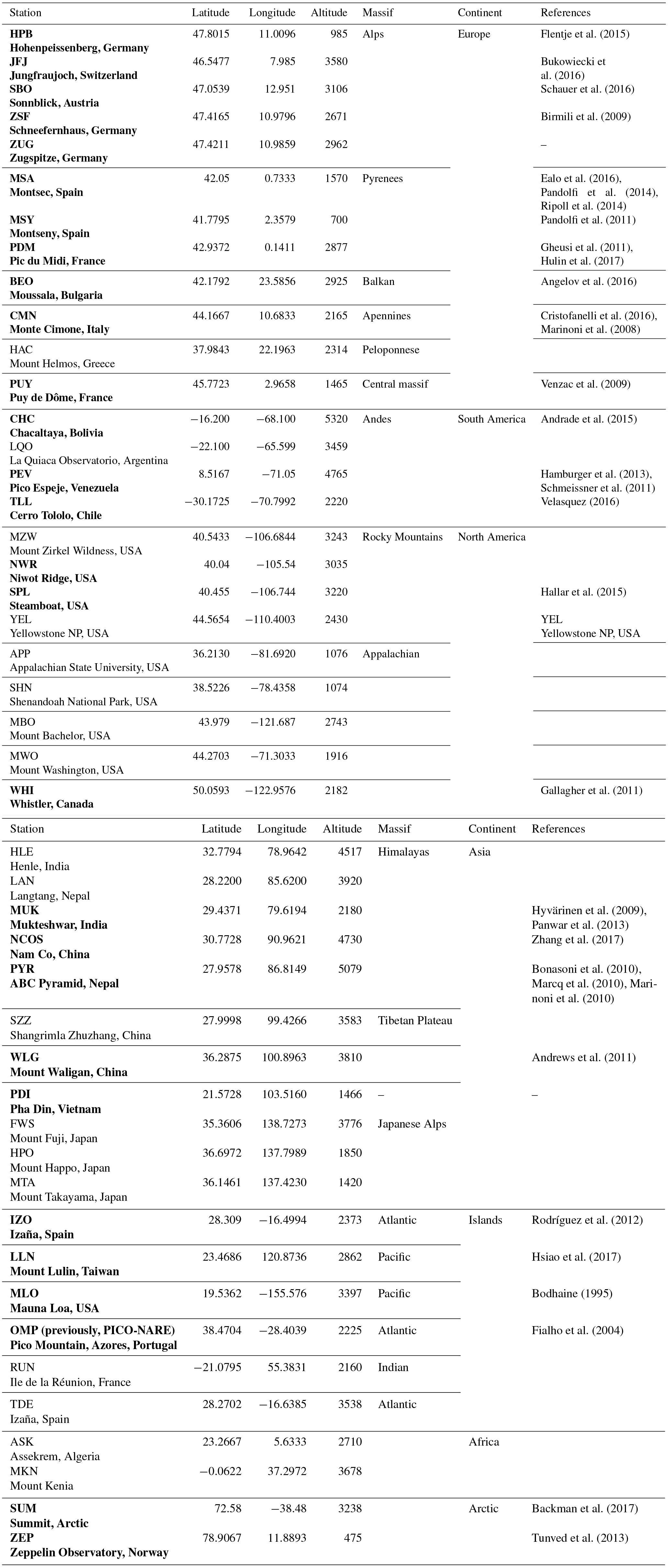
Table 1List of station names, acronyms, latitude [∘], longitude [∘], altitude [m], their mountain range or region and continent. If aerosol time series were used, the station name is given in bold. The references principally describe the station measurement program and, particularly, the aerosol parameters measured.
The altitude range of stations which claim they sample in the FT (at least some of the time) spans from about 1000 to more than 5320 m a.s.l., but a simple analysis of the aerosol parameters (for example, the black carbon concentration) as a function of altitude suggests that higher altitude stations are not necessarily less influenced by anthropogenic pollution than lower altitude sites. While station altitude may not be the main parameter explaining the ABL influence, topographical features around the station are nevertheless involved in the CBL development and in the formation of thermally induced winds leading to ABL air lifting (Andrews et al., 2011; Kleissl et al., 2007). In addition to topography there are other important parameters determining the ABL influence at mountainous stations, such as the wind velocity and direction, soil moisture and albedo, synoptic weather conditions, pollution sources, and, for islands, sea surface temperature, but none of these parameters will be considered in this study, which is solely restricted to the analysis of the topographic influence.
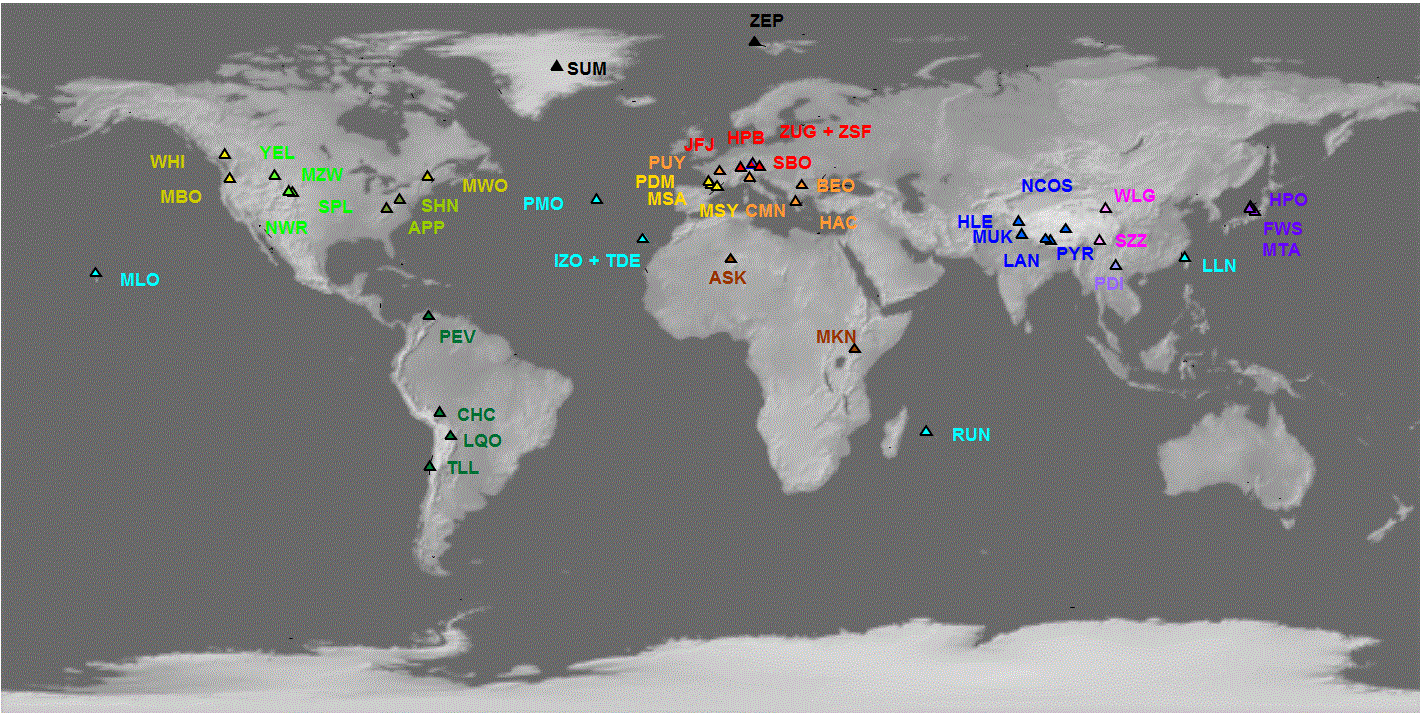
Figure 1Map of the stations colored by their mountain ranges or region. The background topography was taken from http://cartographicperspectives.org/index.php/journal/article/view/cp74-huffman-patterson/623 (last access: 17 July 2018).
The aims of this paper are twofold: (i) define a topography based index called ABL-TopoIndex that can be utilized to rank the high altitude stations as a function of the ABL influence and (ii) compare the potential ABL influence of several locations in a mountainous range in order, for example, to choose the best sampling location for accessing FT air. Some concepts tested or used in this study are taken from the hydrology analysis field, as both air and water flow along defined, though (often) different, flow paths. The ABL air masses flow towards high altitudes and can extend into a three dimensional space, in contrast to the downward flow of water that can be restricted to a two dimensional space. However, similar to hydrological concepts, the ABL air mass reservoirs are found in the plains and valleys.
2.1 Stations
The 43 high altitude stations (Table 1 and Fig. 1) were selected based on various criteria, such as the presence of aerosol or gaseous measurements, their representativeness of the mountainous massif and/or the possibility of comparing several stations from the same mountainous massif. The sites are representative of five continents and their altitudes range between 1074 (SHN) and 5352 m a.s.l (CHC). Note that when not specified, altitudes given in the text correspond to altitude above sea level (a.s.l.). Even if clearly situated within the ABL, some stations like HPB, MSY or ZEP were added to this analysis to verify the results of the ABL-TopoIndex at lower altitude sites. Several mountainous massifs such as the Alps, the Himalayas, the Rocky Mountains and the Andes Cordillera are well represented with three to five stations. Some other stations such as BEO in the Balkan Peninsula, HAC on the Peloponnese, WLG in China, PDI in Vietnam, MKN in Kenya and the high plains of ASK in the Hoggar Mountains of southern Algeria are the only representative of their massif. The volcanic islands form a category in themselves, despite being located in different oceans and at various latitudes.
2.2 Topography data and analysis
The topography data were taken from the global digital elevation model GTopo30 (https://lta.cr.usgs.gov/GTOPO30, last access: 20 August 2018). GTopo30 has a horizontal grid spacing of 30 arcsec corresponding to a spatial resolution between 928 m in the East/West direction at the equator, 598 m at WHI (50∘ N) and 373 m at the SUM polar station (72.6∘ N). In the North/South direction, 30 arcsec are almost constant with latitude and correspond to 921 m at the equator and 931 m at the poles. The geographical coordinate system WGS84 (World Geodetic System revised in 1984) from GTopo30 was projected in the Universal Transverse Mercator (UTM) conformal projection to ensure homogeneity in vertical and horizontal coordinates. Due to the altitude averaging over each grid cell, there is typically an altitude difference between the true station altitude and its corresponding grid location. The mean and median of the differences between the station altitude and its representative grid point are 190 m (8.6 %) and 140 m (5.8 %). For stations situated near the summit, the difference can be significant: five stations have an underestimation of their altitude larger than 500 m corresponding to 15 %–32 % (see the Supplement and particularly Table S1 for further details), despite, according to the manual, the high reported GTOPO30 accuracy (minimum accuracy of 250 m at 90 % confidence level with a RMSE of 152 m).
The TopoToolbox-master version of the free shareware TopoToolbox (https://topotoolbox.wordpress.com/, last access: 20 August 2018), which is a set of matlab functions offering analytical GIS utilities in a non-GIS environment (Schwanghart and Scherler, 2014), was used as a principal tool for the topographic relief and flow pathways analysis in the Digital Elevation Model (DEM) analysis. The DEM were preprocessed by filling holes with a carving process prior to calculating the flow directions and the water flow paths were calculated with single flow direction representation.
2.3 ABL-TopoIndex
To construct the ABL-TopoIndex, we rely on the following four criteria to indicate that the ABL influence will be low if the following criteria are met:
-
the station is one of the highest points in the mountainous massif,
-
there is a large altitude difference between the station and the valleys, high plains or the average domain elevation,
-
the slopes around the station are steep, and
-
the inverse drainage basin, which potentially reflects the source area for thermally lifted pollutants, is small.
Based on these criteria, it can be inferred from Fig. 2 that the “red” station will be less influenced by the ABL than the “blue” station, despite being situated at lower altitude. A quantitative estimation of these criteria clearly depends on the domain considered. The minimal size requirement for such a topographical analysis is that the domain should contain the whole mountainous massif. An airborne lidar measurement of the ABL over the Alps (Nyeki et al., 2002) clearly showed that the convective boundary layer is formed over a large-scale and leads to an elevated and extended layer. Nyeki et al. (2002) also quantified this “large-scale” to extend more than 200 km from the mountainous massif. A rectangular domain size of 500 km × 500 km centered on each site was thus chosen for this analysis (see Sect. 3.2 for a discussion of the effect of the domain size). The four criteria listed above are then represented using five parameters (Table S2 lists topographical and hydrological parameters considered but rejected for this analysis).
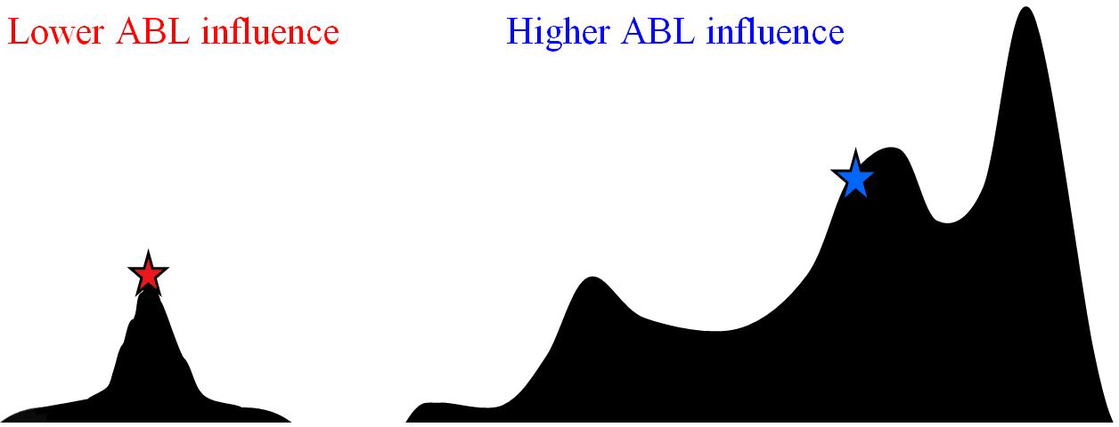

Figure 3(a) Normalized hypsocurves for a selected subset of the high altitude stations for a 500 km × 500 km domain centered on each station. The filled and open circles correspond to the normalized station elevations within the domain and indicate the value of hypso% (e.g., PYR hypso% = 26). The vertical dashed line corresponds to 50 % of the hypsometric curve. (b) Difference between the station altitude and the elevation minimum in a domain of radius R around the station as a function of R. The vertical dashed line indicates the part of the curve selected to calculate LocSlope.
-
Parameter 1 – hypso%. A hypsometric curve is the cumulative distribution function of elevation on the considered domain. The frequency percentage of the hypsometric curve at the station altitude (hypso%) provides a representation of criterion 1 for a large spatial scale (500 km × 500 km). Figure 3a presents several normalized hypsometric curves with dots indicating the station hypsometric value. While most of the high altitude stations (65 %) have hypso% values less than 10 %, some stations are situated on wide inflection points of the hypsometric curve (see, e.g., PYR and NCOS in Fig. 3a). Six stations (see Table S1) have hypso% values larger than 50 %. BEO and FWS are found at less than 0.1 % of the curve indicating they are located at one of the highest points of their respective mountainous massifs. The ABL influence should increase with increasing value of hypso%.
-
Parameter 2 – hypsoD50. The second parameter (hypsoD50) is the difference between the station altitude and the altitude at 50 % of the hypsometric curve. The median of the hypsometric curve was chosen first because a station claiming to be a high altitude site should typically be at a higher altitude than half of its geographical environment and, second, because the median is a commonly used statistical concept to determine the central value of a sample. The parameter hypsoD50 corresponds to criterion 2 for a large spatial scale (500 km × 500 km). In some cases (see Fig. 3a and Table S1), a station is situated under 50 % of the hypsocurve, leading to a negative hypsoD50. For these sites the hypsoD50 is set to the very small value of 1000/abs(hypsoD50) to allow the geometric mean to be applied (see Eq. 1). The ABL influence should decrease with increasing values of hypsoD50.
-
Parameter 3 – LocSlope. The altitude difference between the station and the minima in a circular domain centered at the station is plotted as a function of the domain radius in Fig. 3b. The slope of this curve between 1 and 10 km is then calculated (LocSlope) and corresponds to criteria 2 and 3 for a small spatial scale (10 km × 10 km). The steepness of the slopes (criterion 3) around the station is only evaluated from the station toward the lowest elevations. The distance of 10 km to calculate the LocSlope was chosen as representative of the maximum distance to the next adjacent level region for almost all stations. Figure 3b shows that the change in the altitude difference as a function of domain radius can be very different from station to station. For example, there is a rapid decrease of the altitude difference with increasing distance that gradually levels off for radius larger than 7 km for JFJ and for radius larger than 4 km for MBO; there is a continuous decrease of the altitude difference for PYR and ASK up to radius larger than 30 km; and there are sites for which the altitude difference stays constant for a portion of the domain radius (see for example CHC and BEO) indicating the presence of flat terrain. NCOS appears very different than the other sites plotted because the NCOS station is near the vast Nam Lake (surface area 1950 km2) situated at 4718 m. The ABL influence should increase with decreasing LocSlope.
-
Parameter 4 – G8. The mean gradient in elevation in the eight directions (N, NE, E, SE, S, SW, W, NW) at the station is called G8. This parameter takes into account the slopes towards lower and higher elevations over a local scale (0.5–1.1 km, which is the distance between two grid cells, with the size of the grid depending on latitude) and corresponds to criterion 3. The ABL influence should decrease for increasing G8 gradient.
-
Parameter 5 – DBinv. As the air masses have to be thermally lifted from the valleys and plains towards the summit to influence the station measurements, the size of the inverse drainage basin (DBinv) can be calculated with standard hydrology tools, using an inverse topography, where the altitude Z is changed to −Z, allowing the summit to become a hole. It potentially represents the region from which pollutants such as aerosols can be thermally lifted without crossing any topographical barrier. DBinv is related to criterion 4 for a large spatial scale (500 km × 500 km). Figures 4d and 5d are examples of the DBinv calculation for BEO and PYR. The ABL influence should increase with increasing size of the inverse drainage basin.
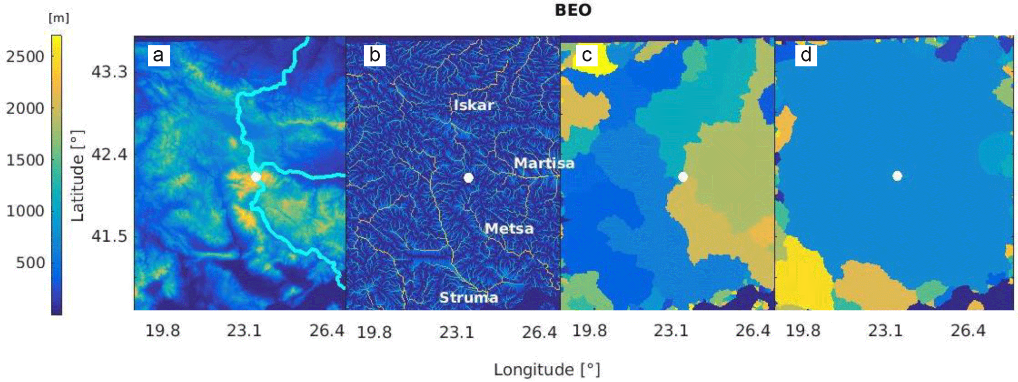
Figure 4(a) Topography on a 750 × 750 km2 domain around BEO (Moussala, white dot) in Bulgaria. The main hydrologic flow paths from the station grid cell are given by the cyan lines. The color scale on the left only applies to panel (a). (b) Hydrographical network and (c) hydrologic drainage basins calculated from the real topography, the different drainage basins are defined by various colors and (d) “inverse drainage basin” calculated from the inverse topography (DBinv).
Table 2Extrema, median and mean of the topographical parameters for the 46 stations studied.
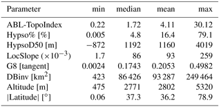
To summarize, the ABL influence should increase with decreasing values of hypsoD50, LocSlope and G8 and with increasing values of hypso% and DBinv. Thus, to determine the ABL-TopoIndex, the geometric mean is calculated on the inverse of hypsoD50, LocSlope and G8 along with the values of hypso% and DBinv. To avoid any particularities of the station site and due to the fact that the ABL influence is a regional factor, the mean of the values at the grid cell containing the station and at the eight neighboring grid cells (recall that grid spacing is 30 arcsec) are used to calculate the ABL-TopoIndex. The ABL-TopoIndex is then taken as the geometric mean of the five parameters:
The geometric mean is used here on strictly positive parameters that have widely different numeric ranges (e.g., Table 2). The geometric mean is used instead of the arithmetic mean because it effectively “normalizes” the various parameter ranges, so that no parameter dominates the weighting. Further, a given percentage change in any of the parameters will yield an identical change in the calculated geometric mean value. In that sense, the variability of each parameter is also normalized, leading to similar modifications of the ABL-TopoIndex for similar parameter's variations. Because of these properties, the geometric mean is the recommended method to determine meaningful indices from multiple parameters (Ebert and Welsch, 2004). The extrema, median and mean of the parameters constituting the ABL-TopoIndex are reported in Table 2. The value of the ABL-TopoIndex has no significance in itself, so that the units are not important, but it allows ranking of the stations as a function of the ABL influence due to convection.
2.4 Aerosol parameters
Aerosol datasets from 25 high altitude and 3 mid-altitude stations (Table 1) were available for this study, 21 of them coming from GAW (Global Atmospheric Watch) stations. The datasets comprise absorption coefficient, scattering coefficient and/or number concentration and cover time periods ranging from at least a year up to more than a decade of measurement (see Table S3 in the Supplement). Stations with time series shorter than one year were not used, as their data are not representative of a complete seasonal cycle. Due to the non-normal distribution of the aerosol parameters, the 5th, 50th and 95th percentiles were taken as representative of the minimum, central position and maximum concentrations.
No correction for standard pressure and temperature was applied in order to use the measured aerosol properties and concentration at high altitude. For consistency, the measured hourly absorption and scattering coefficients were adjusted to a wavelength of 550 nm if reported at a different wavelength using an assumed scattering or absorption Ångström exponent of 1. Additionally, the scattering coefficients were corrected for angular truncation error. Due to the measurement technique and the low aerosol concentrations at many high altitudes, filter-based photometers regularly measure negative absorption coefficients at some of these sites. Some datasets contain up to 20 %–30 % of negative absorption values. Depending on the data owner's policy, these negative values were either left in the dataset, set to zero (or to a minimum value) or considered as missing values. To ensure a similar treatment for all datasets, negatives values, zeros and minimum values attributed to negatives were thus set to missing values.
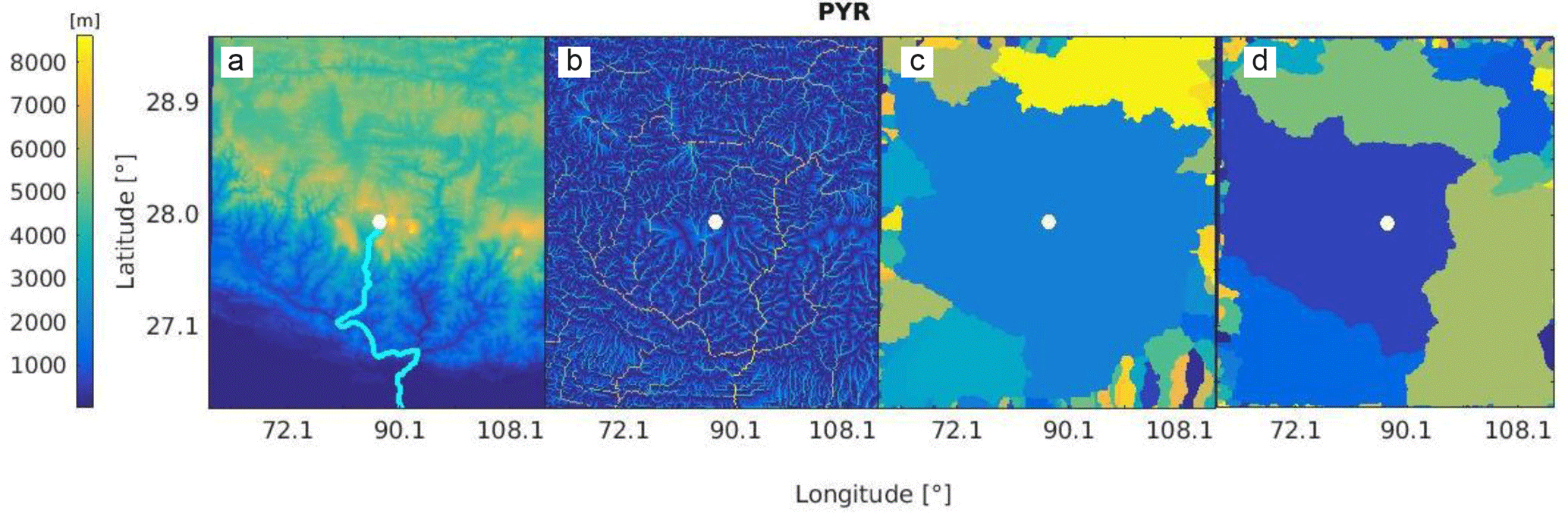
Figure 5The same as Fig. 4 for PYR (Nepal Climate Observatory – Pyramid) station in the Himalaya, Nepal.
The diurnal and seasonal cycles were only analyzed on datasets longer than 2 years. To be able to statistically calculate the diurnal and seasonal cycles, the autocorrelations at 1 h (first lag) were first removed from the dataset by a whitening procedure (Wang and Swail, 2001). The autocorrelations at each lag time were then calculated on the whitened dataset taking into account missing data (see Supplement for further explanations). Only autocorrelation values statistically significant at 95 % confidence level were kept. As the diurnal (24 h) and annual cycles (365 days) were not well defined due to variable meteorological conditions and some shorter datasets, the autocorrelation at lags of 22 to 26 h and at lags of 350 to 380 days were summed to obtain the strength (i.e., the cycle amplitude) of the diurnal and seasonal cycles, respectively. Noise in the aerosol measurements makes the strength of the cycle a somewhat qualitative value. The diurnal cycles were calculated for each month of the year in order to observe the seasonal change of the diurnal cycles.
3.1 Case studies
Mount Moussala (BEO) is the highest summit not only in Bulgaria but of the whole Balkan massif. The regional GAW station is located at the summit (2925 m). The topographic dominance of BEO can be visualized on the topography map (Fig. 4a). Figure 4a also shows the main hydrological flow paths which follow the Iskar, Martisa and Metsa rivers. Figure 4b shows the water flow accumulations, which are the accumulated flows of all cells flowing into each downslope cell in the output raster, allowing visualization of the largest features of the Bulgaria hydrographic network. BEO is at the junction of four drainage basins corresponding to the four main rivers (Fig. 4c). Figure 4d shows that when the inverse drainage basin is calculated with the inverse topography, BEO is in the center of a large inverse drainage basin that covers most of the plotted domain. Even though BEO's altitude is under 3000 m, BEO's ABL-TopoIndex of 0.52 is one of the lowest, due to an almost zero hypso% (0.034 %), a high hypsoD50 of 2136 m and a relatively small DBinv of 1.15×10⁵ (Tables 2 and S2). HAC is a very similar case to BEO as the site is situated near the top of Mount Helmos, the third highest mountain of the Peloponnese massif in Greece.
PYR (5079 m) is the second highest station of all stations considered in this study, but the station is located at the foot of Mount Everest (8848 m) at a confluence point of several valleys (Fig. 5a and b). Figure 5c shows that PYR is situated in the middle of a very large hydrological drainage basin highlighting the fact that the PYR station is not located at a dominant position in the Himalayas. The PYR ABL-TopoIndex is consequently quite high (3.43) and supports the observation of a large ABL influence in the Himalayan region (Bonasoni et al., 2008). The daily arrival of polluted air masses from the Indo-Gangetic plain is frequently reported in PYR data analyses (Bonasoni et al., 2010, 2012; Marinoni et al., 2010).
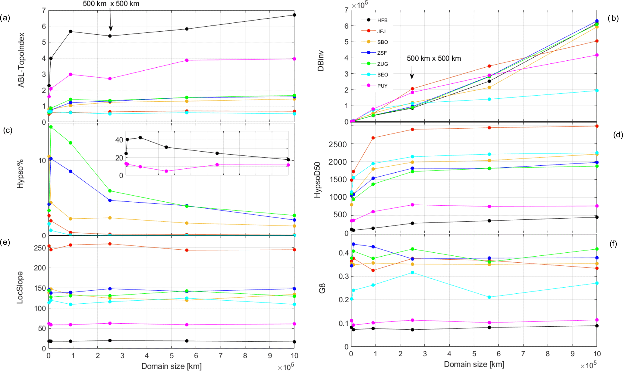
Figure 6(a) ABL-TopoIndex, (b) inverse drainage basin, (c) hypsometric percentage of the station elevation, (d) hypsometric percentage of the station elevation minus the 50 % hypsometry, (e) local slope in a circle of 10 km radius centered on the station, (f) gradient in elevation as a function of the domain size for some European high altitude stations.
3.2 Relation between ABL-TopoIndex and domain size
As the ABL-TopoIndex depends on the size of the chosen domain (Fig. 6a), we have conducted an evaluation of the sensitivity of the various algorithms to the domain size using a range from 50 to 1000 km2. The gradient criterion G8 and the local slope criterion LocSlope are calculated on small fixed horizontal scales (0.5–1 and 10 km, respectively) and are consequently constant with domain size (Fig. 6e, f), although there are small fluctuations due to some distortions occurring during the projection of GTOPO30 in the UTM WGS84 coordinate system, primarily when the analyzed domain extends beyond two UTM zones (see for example BEO). The other three parameters do change with domain size which is the reason that the ABL-TopoIndex also is a function of the domain area. DBinv tends to increase with the domain size for all stations (Fig. 6b), as the size of the low altitude area potentially contributing to thermally lifted pollutants increases with domain size. The hypso% decreases continuously with domain size for stations situated in a dominant position in their mountainous massif such as JFJ, SBO or BEO (Fig. 6c). For stations located at a lower position in their massif (see for example HPB), the hypso% first increases before decreasing once the domain contains all the highest peaks of the massif. Finally, stations situated atop a high local mountain but surrounded by higher mountains such as MUK (not shown in Fig. 6) have a continuously increasing hypso% up to very large domain sizes (106 km2 for MUK). HypsoD50, the difference between the station elevation and the minimum of elevation in the domain, always increases (or at least stays constant) with an increase in domain size but changes more or less rapidly depending on the domain topography (Fig. 6d). In general, the ABL-TopoIndex usually increases with an increase in domain size (i.e., more ABL influence). The largest increases are usually found for the stations with the highest ABL-TopoIndex at small domain sizes and are due to an increase in DBinv overcoming the decrease in hypso% and the increase in hypsoD50.
3.3 Relation between ABL-TopoIndex and altitude
As stated in the introduction, the development of the ABL-TopoIndex relies on the assumption that the station position in the mountain massif is a better criterion for determining the ABL influence than the station altitude alone. To compare these two parameters, we show in Fig. 7 the ABL-TopoIndex as a function of the altitude for all grid cells in a 5 km × 5 km domain for a subset of stations. For the grid cells at the highest altitudes, there is a clear relationship between the ABL-TopoIndex and the altitude. The ABL-TopoIndex decreases (less ABL influence) as altitude increases. Figure 7 shows that the OMP and PYR regions have a very large ABL-TopoIndex decrease with altitude while ASK exhibits a very small ABL-TopoIndex decrease with altitude. At lower altitudes for each massif, the valleys, high plains and various mountainous slopes lead to a wide range of the altitudes corresponding to the same ABL-TopoIndex value. For example, the altitude range corresponding to an ABL-TopoIndex of 3 varies between 3000 and 6000 m at PYR, while at OMP an ABL-TopoIndex of 2 is achieved at an altitude range between 250–350 m. At PYR and CHC, there are discrete groupings of points likely corresponding to the basins of different valleys around the site. The ABL-TopoIndex values of the stations are indicated by the square markers, allowing visualization of their relative situation in their respective mountain massifs: OMP, HAC and CHC and to some extent SBO were located at places with the lowest ABL-TopoIndex of their regions thus minimizing potential ABL influence. In contrast the region around PYR (and to a lesser extent ASK) shows locations with much lower ABL-TopoIndex (less ABL influence) at similar altitudes to the stations.
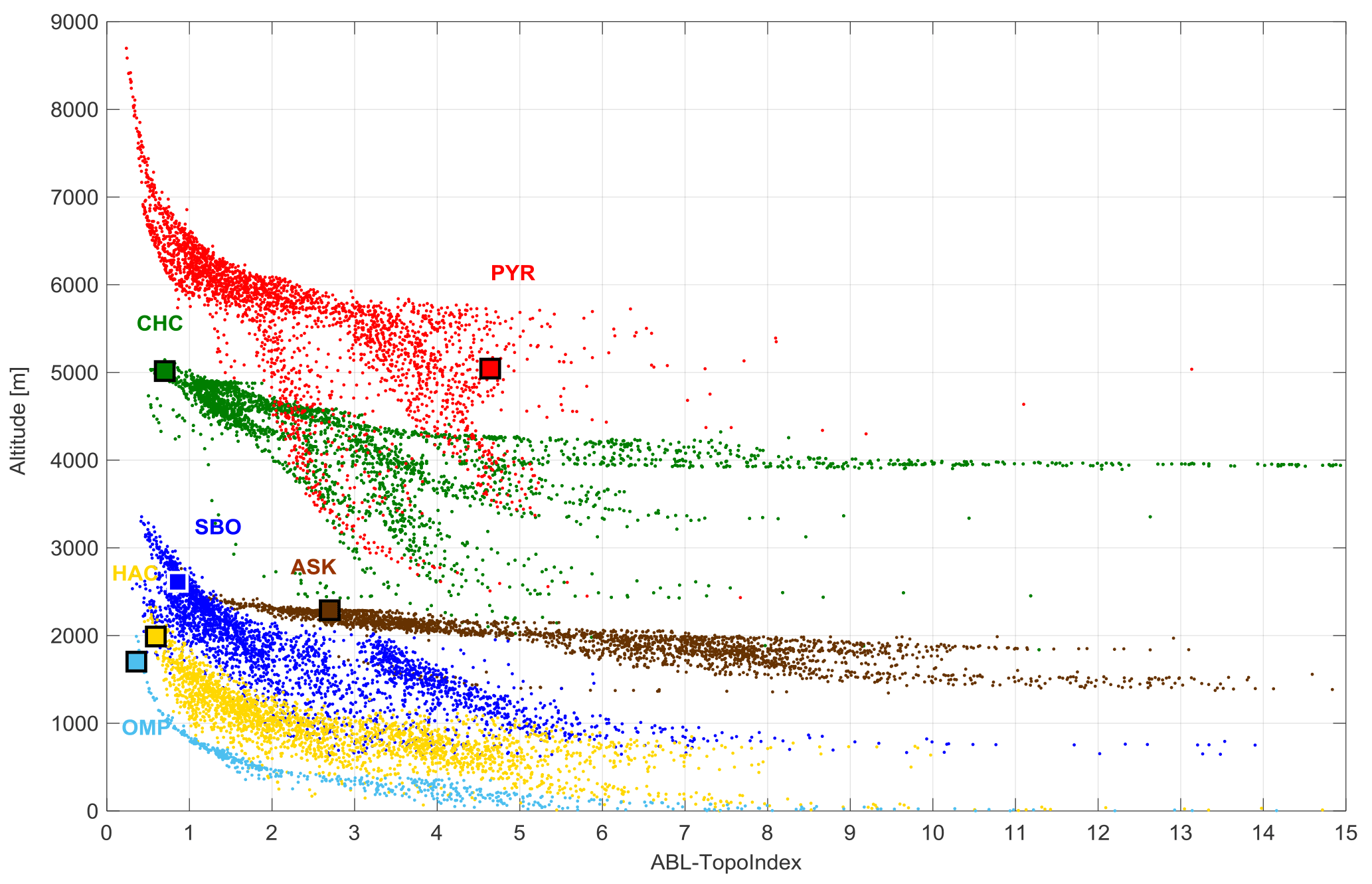
Figure 7ABL-TopoIndex as a function of elevation of all grid cells of a 625 km2 domain centered on the ASK, CHC, HAC, OMP, PYR and SBO stations. The squares indicate the ABL-TopoIndex values and the altitudes of the stations.
3.4 Relation between the ABL-TopoIndex and the station location
The ABL-TopoIndex values for the forty-six stations are grouped as shown in Fig. 8 by continents and mountainous massifs or regions (see Table 1 and Fig. 1) that can correspond to various geomorphologies. The first obvious observation is that all islands have very low ABL-TopoIndex (note the logarithmic scale for the ABL-TopoIndex), whereas the stations in the Himalayan massif have the highest ABL-TopoIndex. The values of the ABL-TopoIndex and of all its constituting parameters are given in Table S1. From this, the following conclusions can be drawn.
Islands. The islands with sites included in this study have a small area, are delimited by the large flat ocean (though most of them are grouped in archipelagos) and their summits were formed by volcanic activity leading to steep slopes. All these factors lead to very low ABL-TopoIndex values. The Teide Observatory on Izaña, an island of the Canary Islands archipelago (TDE) and Pico Mountain Observatory (OMP) in the Portuguese Azores archipelago rank as the monitoring stations with the lowest ABL influence. The low ABL-TopoIndex of both stations is caused by the following reasons: (1) both mountains are the only summit of the island and the highest mountain of their archipelago (3715 and 2350 m, respectively), (2) both islands have small surface area (2034 and 447 km2) and (3) both research stations are just below the mountain summits (177 and 126 m from the summit). The effect of the proximity to the summit can be clearly seen by the difference between TDE (ABL-TopoIndex of 0.22) and IZO (ABL-TopoIndex of 0.57). These two sites, both located on the island of Tenerife, are separated by only 15 km in horizontal distance but a vertical distance of 1165 m, with TDE being the higher station. Taiwan, where LLN is located, has the largest surface area (36 193 km2) of the islands considered here and, additionally, is in close proximity to a continent (China is 130 km to the west). Both of these factors explain LLN's high ABL-TopoIndex in the island category. MLO in Hawaii is at high altitude (3397 m), but the island of Hawaii has a second summit, Mauna Kea (4205 m). Further, the MLO research station is 870 m beneath the volcano top and has a relatively low G8, explaining why it has a higher ABL-TopoIndex than most of the islands. This difference in ABL-TopoIndex between OMP and MLO is confirmed by an almost daily occurrence of buoyant upslope flow at MLO while such flow patterns are much less frequent (<20 % of the time) at OMP (Kleissl et al., 2007).
Alps. The European Alps consist of a broad mountainous massif with the highest summits between 4500 and 4800 m. The four high research stations (JFJ, SBO and ZUG/ZSF) are located between 2900 and 3600 m (ZSF being only some 300 m below ZUG). HPB (985 m) was added to this study as a low elevation station in the Alps. All three high elevation stations have low ABL-TopoIndex: JFJ (0.64), SBO (1.24) and ZUG (1.35). Their ABL-TopoIndex values are generally a little higher than those determined for the islands. As expected, the ABL influence at HPB is much stronger (ABL-TopoIndex is 5.38) due to both its lower altitude and position near the bottom of the Zugspitze massif.
Pyrenees. The Pyrenees are a natural border between France and Spain and peak at 3400 m. PDM is a high altitude station (2877 m) with an ABL-TopoIndex similar to the European alpine high altitude stations. MSA is located at a mid-altitude range of the massif and has a median ABL-TopoIndex, while the low altitude MSY station, added for comparison purposes, has a high ABL-TopoIndex.
Other European stations. BEO and HAC are situated at the highest points of their massifs and thus have very low ABL-TopoIndex values, comparable to those of the island high elevation sites. The lower altitudes of CMN and PUY, their middle position in mountainous massifs containing several higher summits and, to a lesser extent, their proximity to other massifs such as the Alps and the Pyrenees result in higher ABL-TopoIndex values for these two sites.
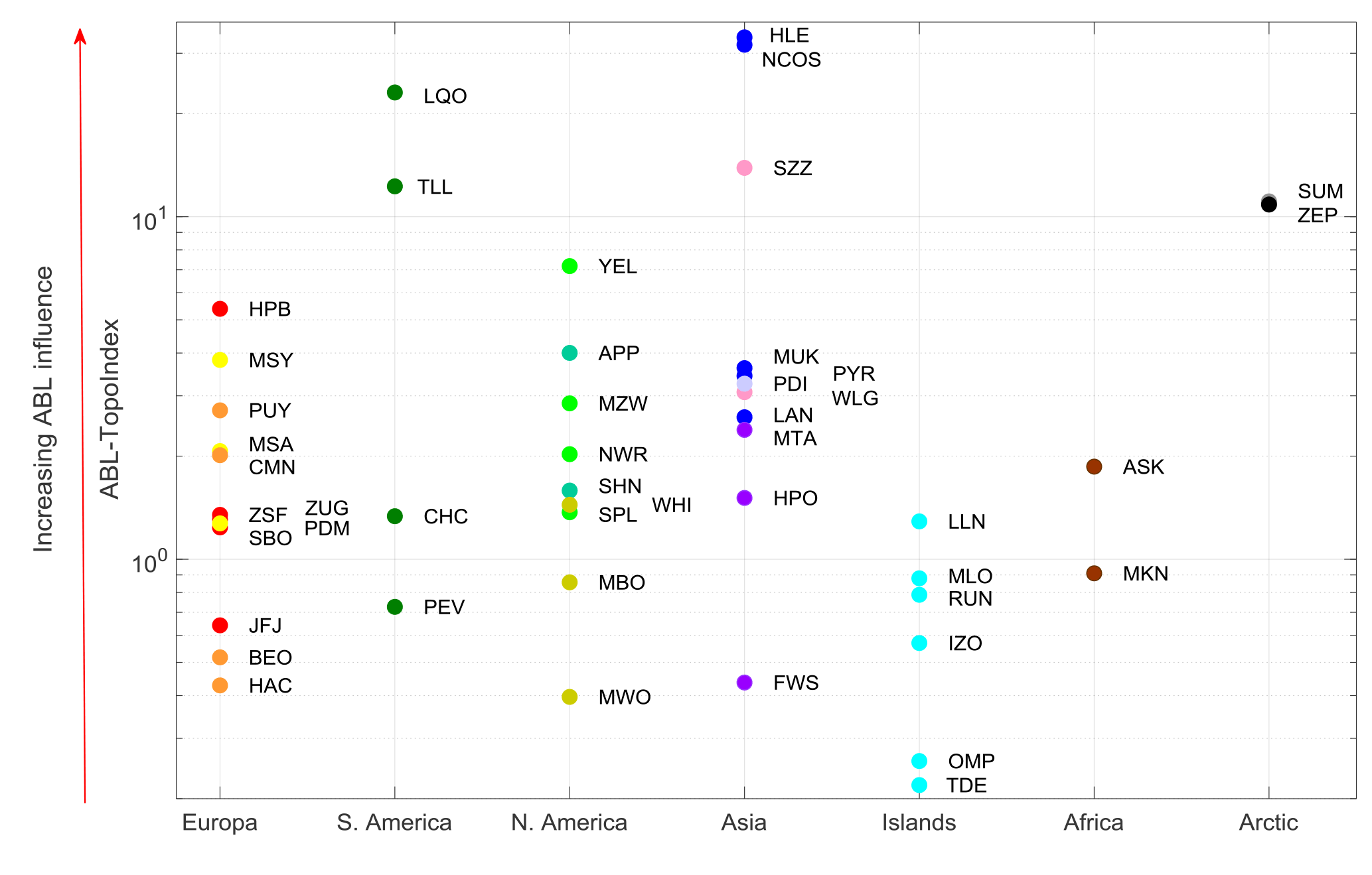
Figure 8ABL-TopoIndex for all stations as a function of continents and mountain ranges. The color scheme corresponds to that in Fig. 1.
Himalayas and Tibetan Plateau. The Himalayas are the highest mountainous massif on Earth with 14 summits peaking at more than 8000 m. The altitudes of the research stations fall between 2200 and 5100 m but are at relatively low elevation in comparison to the summits. This is clearly reflected in their high ABL-TopoIndex values (between 3 and 30). MUK and SZZ are both situated in the foothills of the Himalayas in India (Uttarakhand region) and in south China (Yunnan region), respectively, and both have an ABL-TopoIndex value in the 3–10 range. Although MUK is at a lower altitude than SZZ, it is located at a higher position than SZZ relative to the mean altitude of its meso-scale environment. The high ABL-TopoIndex values for HLE and NCOS are due to their positions in a large valley and on the edge of a vast lake, respectively. Such positioning largely decreases all the parameters related to criteria 1, 2 and 3 (see Sect. 2.3). WLG is constructed within a few meters of Mount Waliguan's summit on the northeastern part of the Tibetan plateau; its dominant position in its meso-scale domain leads to a middle range ABL-TopoIndex value.
Japan. Mount Fuji is the highest peak of Japan and the research station is located at the top of the symmetric volcano located near the coast. The second highest peak in Japan is some 500 m lower than Mount Fuji. This particular topography leads to an ABL-TopoIndex similar to the volcanic islands. The two other Japanese stations are at much lower altitudes and have mid-range ABL-TopoIndex values.
North America. Mount Washington Observatory is located in the Presidential Range of the White Mountains. It is the highest peak in the northeastern United States and the most prominent mountain east of the Mississippi River. MWO is consequently the North American station with the lowest ABL-TopoIndex due to very low hypso% and relatively high G8, LocSlope and hypsoD50. Four stations (MZW, NWR, SPL and YEL) are situated in the Rocky Mountains, whose summits peak at 4400 m. The three stations higher than 3000 m have lower ABL-TopoIndex values similar to some of the European mountain sites, whereas YEL is situated on the wide Yellowstone high plains with an average elevation of 2400 m. Thus, YEL has a high ABL-TopoIndex (7.2) that is similar to the values for NCOS and HLE. Mount Bachelor (MBO) is located near the top of an isolated volcano from the Cascade volcanic arc that dominates the plains surrounding it, explaining its low ABL-TopoIndex. WHI is located in the Pacific Coast Range, the mountain range referring to the vicinity between the high altitude massif and the ocean coast. The highest peaks in the Pacific Coast Range have summits between 3000 and 4000 m (WHI is at 2182 m). WHI has a middle range ABL-TopoIndex (1.4) despite its low altitude due to the proximity of the ocean and to the rather narrow width of the massif (300 km). APP and SHN are both situated at the same altitude in the Blue Ridge Mountains of the Appalachian range. At the latitude of SHN, the width of the Blue Ridge mountain range is much narrower than at APP's latitude. Moreover SHN is almost on the top of the ridge whereas APP is on a high plain. Therefore, SHN has higher G8 and LocSlope and lower hyps% and DBinv, leading to much lower ABL-TopoIndex than is found for APP.
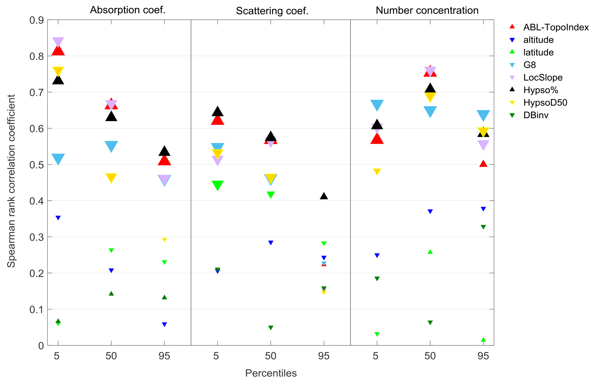
Figure 9Spearman's rank correlation coefficient characterizing the correlation between aerosol parameters (absorption coefficient, scattering coefficient and number concentration) and various topographic parameters (the ABL-TopoIndex, mean altitude over the 9 grid cells, station latitude and the five parameters constituting the ABL-TopoIndex: G8, DBinv, LocSlope, hypso% and hypsoD50). Correlations were calculated for the 5th, 50th and 95th percentiles of the aerosol parameters. Statistically significant correlation values at 95 % and 90 % confidence levels are marked by large and medium symbol sizes and the positive and negative correlations are plotted with upward and downward triangles, respectively. The correlations were performed with 21, 23 and 17 stations for the absorption coefficient, the scattering coefficient and the number concentration, respectively.
Andes. CHC (5320 m), the highest station in this study, is located in the Cordillera Oriental, itself a sub-range of the Bolivian Andes massif, and is part of the mountain bell surrounding the Altiplano (literal translation high plain) with an average height of 3750 m. This position explains its mid-range ABL-TopoIndex of about 1.3 due to relatively high hypso% (1.03 %) and low hypsoD50 (1311 m). PEV (4765 m), the South America station with the lowest ABL-TopoIndex, is located at the extreme northeastern extension of the South America's Andes mountain range that peaks at about 5000 m. Its high position in its mountain range is characterized by a very low hypso% (0.28 %) and the highest hypsoD50 of 4019 m. TLL is situated in the foothills of the Andes in Chile near to the Pacific ocean and has a similar ABL-TopoIndex to SZZ due similarities in topography. LQO is at higher altitude than TLL but located in the middle of the Altiplano leading to an ABL-TopoIndex larger than 20.
Africa. Mount Kenya (5199 m), the second highest peak in Africa and the highest in Kenya, is an isolated volcanic massif with several peaks. MKN observatory is located some 1500 m under Mount Kenya's summit resulting in a mid-range ABL-TopoIndex of about 1. Assekrem (ASK, 2710 m) is located on a small (about 2.5 km2) high plain in the Hoggar Mountains located in central Sahara. The highest summit in the Hoggar range peaks at 2908 m. Despite being situated in a relatively flat area, ASK has quite low ABL-TopoIndex value because of its relatively high elevation in the Hoggar Mountains.
Arctic. SUM is located high atop the Greenland ice sheet in the central Arctic. The ice sheet has a very smooth topography due to its build up by glaciation and precipitation. While SUM has a high hypso%, its hypsoD50, G8 and LocSLope are very low and its DBinv is large, leading to high ABL-TopoIndex. The Zeppelin Observatory (475 m) in Svalbard is located near the top of Zeppelinfjellet (556 m), above Ny-Ålesund, but cannot be considered as a high altitude site and was added to the study for comparison purposes. Its ABL-TopoIndex is consequently very high as the highest summit on Spitzbergen Island is at 1717 m.
3.5 Correlation between aerosol parameters and the ABL-TopoIndex
While Fig. 8 shows that there are some clear patterns in the ABL-TopoIndex, it is also instructive to see how the ABL-TopoIndex relates to measurements at mountain sites. The NCOS and SUM stations have a very high ABL-TopoIndex due to their situation on a high altitude plain near a vast lake and on the smooth shape of the Greenland inland ice sheet, respectively. As they are not situated in a complex topography, they were excluded from this analysis due to their clear outlier status. ZEP, situated at very low altitude (475 m) and very high latitude (78.9∘), also has a very high ABL-TopoIndex value. It was also not included in the correlation analysis as its seasonal and diurnal cycles exhibit different features than the high altitude or middle latitude stations (see Sect. 4.1). In order to have a robust estimate of the correlation between the aerosol measurements (following a Johnson distribution) and the topographical parameters (following a normal or a log-normal distribution depending on the parameter) the Spearman's rank correlation was calculated. It should be noted that the Kendall's tau correlation analysis leads to the same conclusions (see Table S4). The Spearman's rank correlation measures the strength and direction between two ranked variables without the requirement that the variables are normally distributed. Here it is also used to verify that the assumed relationships between topographical and aerosol parameters correspond to those proposed in Sect. 2.3 (e.g., that a positive correlation with aerosol loading as a surrogate for ABL influence in the case of lifting processes without precipitation is found for the ABL-TopoIndex, hypso%, DBinv and station altitude and an anti-correlation with aerosol loading is found for hypsoD50, LocSlope and G8). The expected positive or negative correlations with aerosol parameters are found for ABL-TopoIndex and all five topographical parameters contributing to the ABL-TopoIndex. The Spearman's rank correlation coefficients of the 5th, 50th and 95th percentiles of the measured aerosol parameters with site altitude latitude, ABL-TopoIndex as well as all the individual parameters constituting the ABL-TopoIndex are presented in Fig. 9. (Similar to the ABL-TopoIndex calculation, the mean of the altitudes of the grid cell containing the station and its eight neighboring cells was used.)
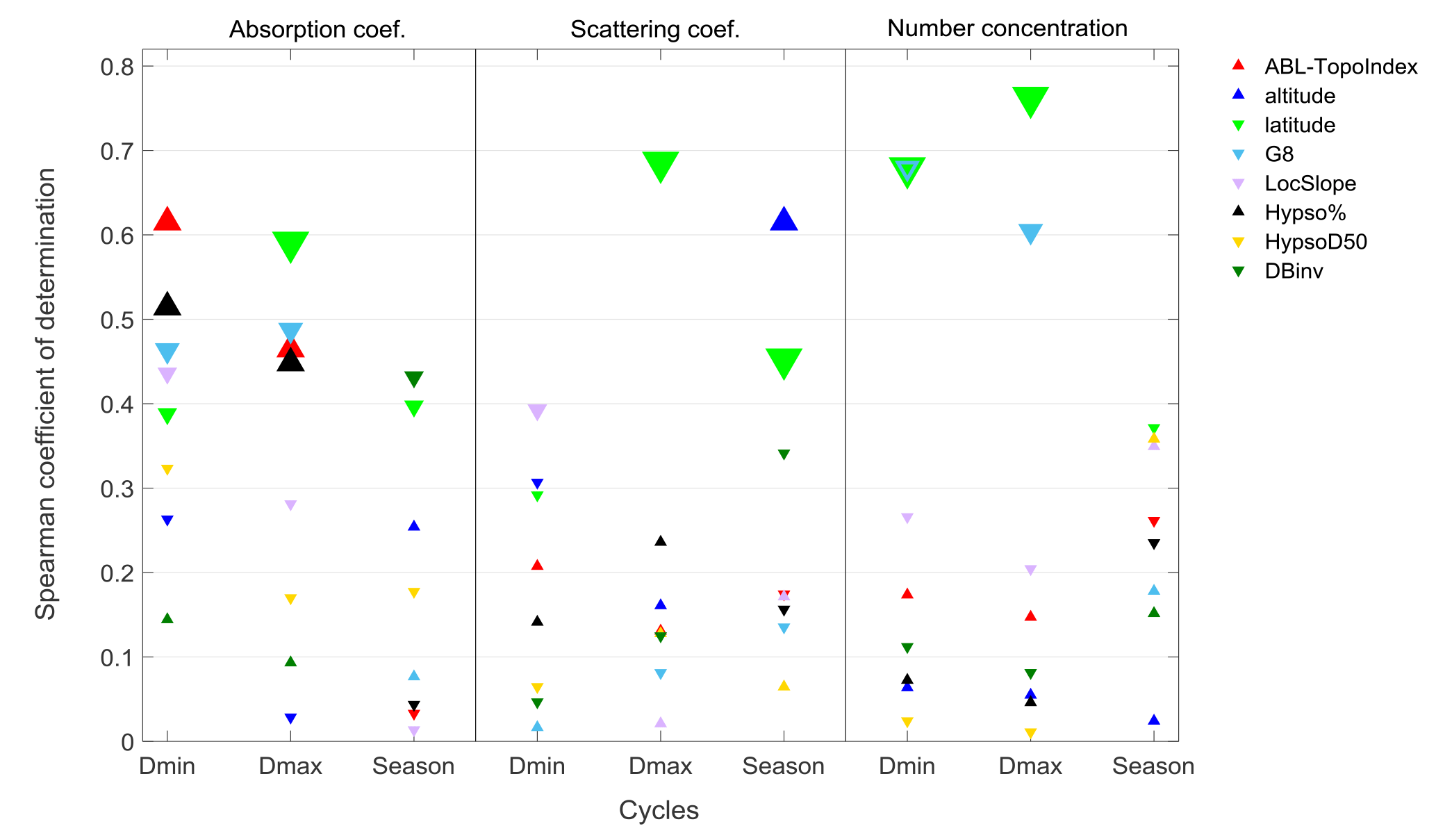
Figure 10Spearman's rank correlation coefficient characterizing the correlation between all the topographic parameters (see Fig. 9) and the minimum and the maximum of the monthly diurnal cycles, as well as the seasonal cycle of the aerosol parameters. The correlations are performed with 21, 22 and 15 stations for the absorption coefficient, the scattering coefficient and the number concentration, respectively.
The ABL-TopoIndex has statistically significant (SS) correlation for all of the percentiles of all aerosol parameters except for the 95th percentile of the scattering coefficient. The highest correlation and SS are found for the fifth percentile of the absorption and scattering coefficient, whereas for number concentration the ABL-TopoIndex is most highly correlated with the 50th percentile. The correlation coefficient of ABL-TopoIndex with the maximum of the aerosol parameters (95th percentile) is always lower than with the minimum (5th percentile) and is SS at 95 % of confidence level only for the absorption coefficient. The fifth percentiles of the aerosol parameters, particularly of the absorption coefficient, correspond to the measurement of air masses with the lowest aerosol concentration, namely FT air masses with the lowest ABL influence and no advection of polluted air masses. In contrast, the 95th percentiles correspond to the advection or convection of air masses with high aerosol loads and can, to some extent, be caused by special events such as dust or biomass burning events. In contrast to the absorption coefficient, the particle number concentration (and, to a far lower extent, the scattering coefficient) depend not only on the ABL influence but also on the new particle formation (NPF) that can be enhanced at high altitudes (Boulon et al., 2011; Rose et al., 2015). Thus, the high correlation of the ABL-TopoIndex with the fifth percentile of the aerosol absorption coefficient as well as lower correlation with the 95th percentile of absorption coefficient, the fifth percentile of number concentration and the 95th percentile of scattering coefficient suggest the ABL-TopoIndex is indeed a promising indicator for ABL influence based on station topography.
The hypso%, a large scale parameter, has SS correlations with all the percentages of all the aerosol optical properties, whereas LocSlope and G8, two small scale parameters, have SS anticorrelations except for the 95th percentile of the scattering coefficient where no SS correlations are observed. The hypsoD50 is SS for the 5th and 50th percentile of the absorption and scattering coefficients and for the 50th and 95th percentile of the number concentration. Only the DBinv exhibits no SS correlation with any of the aerosol parameters.
There are no SS correlations between the station altitude and the percentiles of any of the aerosol parameters. The station elevation alone is thus not a good predictor of the ABL influence (at least as it relates to particle concentration and aerosol optical properties). The latitude is SS anticorrelated with the 5th and 50th percentile of the scattering coefficient.
The correlations of the topographical parameters with the strength of the diurnal and seasonal cycles of the aerosol measurements exhibit a different pattern. Figure 10 shows the Spearman's rank correlation coefficients of the topographical parameters with the minimum (Dmin) and maximum (Dmax) strength of the monthly diurnal cycle as well as with the strength of the seasonal cycle (Season) of the aerosol parameters. The diurnal cycles were calculated for each of the 12 months, so that Dmin and Dmax correspond to the lowest and the highest monthly amplitudes, respectively. For many mountain sites, Dmin occurs when the station remains in the FT during the whole day resulting in no systematic diurnal cycle. In contrast Dmax occurs when the site is in the FT during the night (without any influence of the RL) and influenced by the ABL during the day. The diurnal and the seasonal cycles were both calculated as the strength of the autocorrelation function (see Sect. 2.4 and Supplement) so that the underlying parameters are de facto normalized and that the cycles of each station can be directly compared. The highest correlation (a negative correlation) is found between the amplitudes of the diurnal cycles and the latitude for all three aerosol parameters. This anticorrelation is particularly noticeable for the number concentration diurnal cycles. At low latitudes, the stronger insolation enhances the surface temperature and the thermal convection leading to stronger diurnal cycles, particularly in summer, while the convective flow is less likely to be inhibited during the winter due to longer daylight hours. Together these effects result in a larger ABL influence year round and explain the high correlations of latitude with the diurnal cycle amplitude. The high correlation between the maximal diurnal cycle and the number concentration can also be explained by the promotion of NPF due to the stronger insolation at low latitude.
The ABL-TopoIndex is SS correlated with the minimum and the maximum of the monthly diurnal cycles of the absorption coefficient. This correlation is, once again, primarily due to the hypso% and G8, and to a lesser extent, the LocSlope. The highest correlation is found for the absorption coefficient which directly depends on uplift of ABL air masses, in contrast to the number concentration and scattering coefficient cycles which are also influenced by gas-to-particle conversion processes such as NPF. As NPF can be enhanced at low temperature, (i.e., NPF seasonal cycle can be anticorrelated with the seasonality of the CBL height) the relationship between number concentration (and, to a lesser extent, scattering) with diurnal cycle strength may be obscured by seasonal changes in atmospheric dynamics.
The only SS correlation with station altitude is found for the scattering coefficient seasonal cycle. Similar to the anticorrelation of G8 with the aerosol parameter percentiles, there is also a high anticorrelation between the particle number concentration diurnal cycles and G8 suggesting that the local slope steepness inhibits both the transport of polluted air masses and NPF. Apart from a correlation at 90 % confidence level between DBinv and the absorption coefficient, the lack of further SS correlations for topographic parameters with the aerosol parameter seasonal cycles can be attributed to several factors: (i) the relatively small time period (2–5 years) covered by most of the datasets leading to difficulties in the statistical determination of a yearly periodicity due to inter-annual variability, (ii) the low aerosol concentration at high altitude sites often resulting in measurements near the detection limits of the instruments (see for example the problem with the absorption coefficient at Sect. 2.4), (iii) the seasonal long-range transport effects masking ABL transport and (iv) the necessary whitening procedure (see Supplement) increasing the dataset noise.
In this section the assessments, improvements and applications of the ABL-TopoIndex are discussed. First the possible parameters and phenomena enabling the estimation of the ABL influence are summarized and the occurrence of diurnal and seasonal cycles as a function of the station elevation are discussed. Second, the significance of the correlations between the topographical and the aerosol parameters are further interpreted. Finally, possible additional parameters that could increase the significance and the application of the ABL-TopoIndex are mentioned, in addition to the criteria relevant for choosing future sites to sample FT air masses.
4.1 Using measurements to assess the ABL influence
In order to test the relevance of the ABL-TopoIndex, it is first necessary to find a parameter commonly measured at high altitude stations that can be used as an ABL tracer. Pollutants emitted at the Earth's surface and having a (typically) minimal concentration in the FT could act as potential tracers of the ABL influence. Our results showed that of the three aerosol parameters tested in this study (number concentration, absorption coefficient and scattering coefficient), absorption coefficient has the highest correlation with the ABL-TopoIndex values. Other possible candidates for testing the ABL-TopoIndex include the aerosol mass concentration, size distribution and chemical composition, the water vapor and the trace gases concentrations (e.g., CO2, PAN, NOx, NOy, O3, SO2, isotopologue ratio of water vapor) and the radon222 concentration. These parameters have been used in different studies to provide information about the seasonal and diurnal cycles (e.g., Collaud Coen et al., 2011; Griffiths et al., 2014; Marinoni et al., 2010; McClure et al., 2016; Okamoto and Tanimoto, 2016; Pandolfi et al., 2014; Ripoll et al., 2015; Zellweger et al., 2009), the sources and transport of aerosol to the site (e.g., Cuevas et al., 2013; García et al., 2017; Pandey Deolal et al., 2014; Ripoll et al., 2014), the local orographic flows and the effect of the synoptic- and meso-scale weather types (e.g., Bonasoni et al., 2010; Gallagher et al., 2011; González et al., 2016; Henne et al., 2005; Kleissl et al., 2007; Tsamalis et al., 2014; Zellweger et al., 2003). All of the extensive aerosol parameters, the radon222, water vapor concentration, particulate nitrate () and organics have been shown to be correlated with ABL transport whereas CO ∕ NOy and NOx ∕ NOy ratios are anticorrelated (Legreid et al., 2008; Zellweger et al., 2003). Zellweger et al. (2003) concluded that, in contrast to NOy, the major process for upward transport of aerosol is the thermally induced vertical transport, confirming that the aerosol parameters used in this study could, in most cases, be good tracers for ABL influence. However, one has to keep in mind that many lifting processes co-occur with precipitation and, hence, potential aerosol washout. The present validation of the ABL-TopoIndex by aerosol measurements at high altitude stations is consequently valid only for thermally induced processes without precipitation. ABL events involving air masses with low aerosol concentrations due to washout – for example synoptic lifting or foehn – were not directly analyzed.
Because there are variable pollution levels in the vicinity of the stations, a single absolute value of a pollutant cannot be used to evaluate the ABL-TopoIndex (or ABL influence in general) when considering multiple high altitude stations. An inventory of the proximate pollution sources constraining simulations with meteorological models able to explicitly resolve the role of fine resolution orography would be required before using absolute pollutant concentrations as indicators of ABL influence at high altitude sites. Another possibility would be to weight the pollution source inventories by factors depending on their vertical and horizontal distances to the high altitude stations, as well as on a seasonal parameter representing the potential ABL height. A further use of DBinv to restrict the area of potential pollution sources can also be envisaged, as this parameter describes the domain from which pollutants can reach the high altitude station by convection without crossing topographical barriers. The identification of pollution source areas potentially affecting the high altitude stations can be avoided by instead considering dynamic parameters such as the temporal cycles of various pollutants.
At most of the high altitude stations, a seasonal cycle in ABL-indicator species is frequently observed. The maximum values of the seasonal cycles are often correlated with ABL transport and typically occur in summer or in the pre-monsoon season, while the minimum of the seasonal cycle occurs in winter or monsoon seasons. Usually, at high altitude stations, the spring leads to higher aerosol loading than the autumn; this is probably related to higher ABL height in the spring. These seasonal cycles are explained by the stronger thermal heating of the soil, which induces convection and buoyancy in summer and by the atmospheric cleaning effect of precipitation during the monsoon. It would be expected that stations continuously situated in the ABL throughout the year could exhibit different seasonal cycles than high altitude sites due to the seasonal modification of the sources and/or of the synoptic and meso-scale meteorological conditions (see for example the difference between HPB and JFJ in Fig. S2). In contrast, a station located such that it is continuously impacted by FT air masses or with weak seasonal cycle of the ABL influence would have a seasonal cycle that depends mostly on long-range, high altitude transport climatology, e.g., long-range transport of Asian dust and pollution at MLO in spring (Collaud Coen et al., 2013), North-America ABL transport to IZO through westerlies in spring (García et al., 2017), and dust events in EU spring and autumn (Collaud Coen et al., 2004). As seasonally changing parameters (e.g., temperatures, cloud cover, solar radiation, wind speeds, surface albedo, precipitation) were not studied and as the length of most of the time series were too short to smooth these effects, the ABL-TopoIndex will probably not represent an overall picture of ABL influence except at seasonally invariant sites (e.g., very low latitude sites).
The typical diurnal cycle of ABL pollutants at high altitude stations that are partially influenced by the ABL consists of a minimum in the early morning (04:00–06:00 LTC) followed by an increase of the compound with a maximum in the late afternoon (15:00–17:00 LTC) and a decrease during the night. If the ABL influence is mostly due to orographic winds, upslope or valley winds begin to flow some hours after sunrise and downslope or mountain winds initiate after the occurrence of negative vertical heat flux. Stations always situated in the FT should exhibit no systematic diurnal cycles, whereas the stations always situated in the ABL often show various diurnal cycles that can be explained by the behavior of local sources, the diurnal cycle of the ABL height and/or local meteorological conditions. At high elevation and high latitude stations the diurnal cycle typically vanishes during winter but is clearly present during summer, spring and, to a lesser extent, autumn. For stations at lower altitude that stay in the ABL (or CBL, SBL or RL) during the whole day in summer (e.g., MSA, Pandolfi et al., 2013; HPB and PUY, Hervo et al., 2014), the diurnal cycle may also vanish during that period.
Testing the ABL-TopoIndex using pollutant diurnal cycles is further complicated by the presence of the residual layer (RL) that keeps the pollutants brought to high altitudes during the previous days at those elevated levels during the nighttime. The climatology of the RL height usually exhibits a similar seasonality as the ABL height, with a maximum in summer (or pre-monsoon) season and a minimum in winter (Birmili et al., 2009, 2010; Collaud Coen et al., 2014; Wang et al., 2016). Further, the RL has a similar dependency as the ABL on latitude, i.e., the RL's maximum height also depends on the duration of the incoming radiation. The RL pollutant concentrations are much higher than nighttime FT concentrations, leading to less marked diurnal cycles in summer than in spring (Blay-Carreras et al., 2014; Collaud Coen et al., 2011; Hallar et al., 2016; Hervo et al., 2014). The impact of the RL on the aerosol concentration is probably one of the most important reasons for the low correlation between the topographical parameters and the aerosol temporal cycles. However, the statistical determination of the diurnal and seasonal cycle amplitudes suffer from several difficulties: (1) the low aerosol concentrations observed at high altitude often result in measurements near the detection limit leading to large uncertainties, (2) the high hourly autocorrelation of the data requires a pre-whitening procedure (see Supplement) in order to be able to detect the diurnal and seasonal cycle, (3) meteorological conditions (e.g., cloud coverage, precipitation, seasonal fluctuations, etc.) modify the clear-sky diurnal cycles. These factors constraining the observation of clear statistical temporal cycles in the measurement data also contribute to the observed low correlations between the diurnal and seasonal cycles of the aerosol parameters and the ABL-TopoIndex.
Recently, the influences of the local and of the more regional or meso-scale ABL at the JFJ were separated by differentiating the Local Convective Boundary Layer (LCBL) height from the high altitude aerosol layer (Poltera et al., 2017). The LCBL was found to rarely influence the JFJ research station (never in winter, 4 % of the time in summer corresponding to 22 % of the days with ABL influence), whereas the continuous aerosol layer has a large influence on the JFJ pollutant concentrations (21 % of the time in winter and 41 % of the time in summer corresponding to 77 % of the days with ABL influence). This suggests that the mechanisms explaining the heights of the LCBL and the more horizontally extended aerosol layer have different causes and do not follow the same diurnal pattern. This phenomenon will be more pronounced at continental high altitude stations than at marine isolated island stations since the marine ABL is less prone to strong diurnal cycles.
4.2 Correlation between the topography and the aerosol parameters
The correlations between topographical and aerosol parameters presented in Sect. 3.5 can now be further discussed in light of the pollutant temporal cycles. The absorption coefficient is primarily due to the presence of black carbon emitted from combustion processes occurring mostly in the ABL and rarely near the high altitude stations; additionally, BC aerosol is not produced by any secondary processes. Among the aerosol parameters studied here, the absorption coefficient is thus the best tracer for anthropogenic pollution and biomass burning and consequently for ABL influence. It is thus expected that a better correlation will be obtained between the topography parameters increasing the ABL influence and the absorption coefficient. The ABL-TopoIndex reflects this correspondence, particularly through the contribution of the hypso% parameter (recall that hypso% represents the relative altitude of a station in its mountain range), the LocSlope and G8. The best correlation for both ABL-TopoIndex, hypso%, Locslope and hypsoD50 are found for the fifth percentile of the absorption coefficient, since the minima of the aerosol loading is a better tracer of the lowest ABL influence, whereas the maxima is much more dependent on source intensity and special events. Similar to this result, a clear correlation was also found between the continuous aerosol layer maximum height and the absorption coefficient measured in situ at the JFJ (Fig. 8 in Poltera et al., 2017). The absorption coefficient amplitudes of the diurnal cycle are also the only aerosol cycles having a SS correlation with the ABL-TopoIndex.
It is more difficult to directly tie scattering and number concentration to the ABL incursions. This is because the formation of new particles and their subsequent growth are well-known to be very efficient processes at high altitudes due to the high insolation and the low temperature. Moreover, the NPF is also enhanced by local thermal winds and forced convection due to favorable changes in thermodynamic conditions (Boulon et al., 2011; Rose et al., 2015). It was found at the JFJ and confirmed at other stations that new particle formation, and particularly strong nucleation events, occur mostly when the air masses were in contact with the ABL within 2 days before arriving at high altitudes (Bianchi et al., 2016). NPF and subsequent growth of the particles have a large impact on the number concentration and its temporal cycles and a smaller influence on the scattering coefficient. The parameters describing the local topography (G8 and LocSlope) have the highest correlation with the number concentration and are probably more relevant to the local CBL transport than to the longer range continuous aerosol layer as defined in Poltera et al. (2017). The number concentration and, to a lesser extent, the absorption coefficient percentiles and diurnal cycles are anti-correlated with the local (G8: 0.5–1 km) and regional (LocSlope and hypsD50: 10 km) slopes, suggesting there is an increase of particle number concentration when there are small altitude differences and gentle slopes around the station. This dependence on the ease of local transport can be explained by transport to the station not only of aerosol, but also of gaseous precursors for NPF and of newly formed particles at lower elevations. The higher correlation of local slope (G8 and LocSlope) with the 50th percentile of number concentration rather than with the absorption coefficient can be explained both by the sources of black carbon being very few in the vicinity of most of the high altitude stations and by the smooth pressure decrease experienced by the precursors during their upslope transport along gentle slopes leading to more condensation processes and nucleation.
The aerosol diurnal cycles are influenced by numerous phenomena (see Sect. 4.1) leading to a non-trivial relationship with the ABL influence. The study of the diurnal cycles can bring valuable results if specific cases are analyzed and compared. The statistical approach used here is confounded to the noise in the data (low aerosol concentration and whitening process), to the inter-annual variability of the meteorological processes and to cloud, precipitation and long-range advection involving a large day to day variability. There are consequently few statistical correlations between topography parameters and the diurnal cycles. The clearest correlation is the influence of the insolation on the aerosol diurnal cycles amplitudes. This dependence between the latitude and the aerosol concentration has been noted by Kleissl et al. (2007) and is easily understandable, as the convection and the new particle formation are directly dependent on the solar radiation intensity. However, the other correlations found between some topography parameters (ABL-TopoIndex, hypso%, G8 and LocSlope) and the absorption coefficient are directly tied to the ABL influence.
4.3 Improving and applying the ABL-TopoIndex
The choice of the five parameters included in the ABL-TopoIndex was initially based on several assumptions relating the topography to the ABL influence (see Sect. 2.3). Several other parameters taken from the topography, morphology or hydrology fields such as the topographical wetness index, the upstream catchment area, the Efremov–Krcho landform classification, the integral and index of the hypsometric curve and the topographic prominence were tested but eliminated as being not relevant for various reasons (Table S2). Indeed, most of the parameters comprising the ABL-TopoIndex exhibit some correlations with aerosol parameters. The hypso%, LocSlope and G8 are the parameters explaining the highest variance in the aerosol optical properties, with the hypsoD50 having a lower influence than the other three parameters. It also seems evident that the topographical parameters linked to the steepness and the altitude differences (G8 and LocSlope) are clear indicators for NPF. The DBinv seems to be the least explanatory parameter in terms of ABL influence and this large scale parameter should probably be combined with a source inventory to increase its relevance for identifying boundary layer influence (see Sect. 4.1). However, DBinv does have a clear influence on the statistical significance of the correlations between the ABL-TopoIndex and the aerosol cycles (not shown in the paper) and has the highest correlation with aerosol seasonal cycles. However, the aerosol parameters and, particularly, the absorption coefficient cannot be considered as unique tracers of the ABL, particularly in case of lifting processes with precipitation. Analysis of other ABL marker (gaseous species, radon, wind turbulence, etc.) can provide information on additional transport mechanisms, which would allow for refinement of this topographic analysis by adding further parameters. East-oriented slopes are heated early during the day and thus have a larger contribution to the thermal convection and the associated valley winds. A parameter weighting the east slope area could thus be added to the ABL-TopoIndex. The various geomorphologies of the mountainous ranges included in this study also raise the question of whether the stations should all be combined together for analysis as was done here, or if a morphological parameter should instead be found for each massif. The mountain steepness (at larger scales than LocSlope and G8) also determines the necessary velocity for the wind to cross the mountains and could be an additional parameter. Finally, future studies should attempt to build a direction dependent ABL-TopoIndex that also takes into account the topography of each valley up to the meso-scale range.
It is important to understand the FT vs. ABL influence on historical data sets from established high altitude observatories. The ABL-TopoIndex is one tool that can help elucidate the different influences. A further improvement could include an angular dependency of the ABL-TopoIndex allowing quantification of the potential direction of the maximum ABL influence and the pollutant sources with the largest influence. The ABL-TopoIndex may also be useful a priori in locating measurements for a field campaign or identifying potential sites for long-term observatories if FT measurements are the goal, particularly when no previous measurements exist. For example, in situ aerosol measurements are done at IZO at an altitude of 2373 m, whereas aerosol optical depth and water vapor isotopologues measurements are done at TDE at 3538 m on the same volcano. TDE has a much lower ABL-TopoIndex than IZO and consequently TDE's measurements are more likely to represent the FT. The topography around the PYR station suffers from several factors (see Fig. 7 and Sect. 3.1) leading to a high ABL influence. Even if the choice of the actual site is driven by compelling and practical logistical arguments, other positions at similar altitudes in the massif would have ensured lower pollution impact than is observed at PYR. Finally, some stations such as BEO (2925 m), HAC (2314 m) and MWO (1916 m) are not situated at very high altitudes but present excellent locations for FT sampling. Obviously there are other issues to consider when deploying instruments as well (e.g., ease of access, power availability, presence of local pollution sources, etc.), but the ABL-TopoIndex is one factor that could be considered to maximize the potential for FT sampling.
The ABL-TopoIndex is a topographical index based on the hypsometric curve, the slope of the terrain around the station and the inverse drainage basin that potentially reflects the source area for thermally lifted pollutants. It allows one to rank the high altitude stations as a function of their ABL influence or to optimize choice of site location for FT sampling. High altitude stations situated on volcanic islands, the highest stations in the Alps, in the Andes and in the Pyrenees have low ABL-TopoIndex values. Stations situated at or near the summit of their mountainous ranges such as BEO, HAC and MWO also have low ABL-TopoIndex values. Stations situated at altitudes between 4000 and 5500 m in the Himalayas and the Tibetan Plateau have high ABL-TopoIndex values due to their relatively low position compared to the summits. Statistically significant correlations between the ABL-TopoIndex and the aerosol parameters measured at high altitude sites allowed validation of the methodological approach. The highest correlations are found with the fifth percentile of the aerosol parameters representing the minimal ABL influence or, in other words, the most likely FT air masses. The 95th percentiles of aerosol parameters are more representative of the intensity of aerosol sources and of advection of air masses with high aerosol concentrations. There are also strong anticorrelations between the local steepness of the slope and the particle number concentration, suggesting that new particle formation could be largely influenced by this topographical parameter. If high altitude stations undergo daytime ABL air influence due to convection, a pronounced diurnal cycle of aerosol parameters is usually observed. The amplitude of the diurnal cycle of the absorption coefficient is SS correlated with the ABL-TopoIndex and is thus likely to be representative of ABL influence. However, the strength of the diurnal cycles of the scattering coefficient and the number concentration is mostly explained by the latitude of the station, leading to the conclusion that the solar radiation intensity and duration drive the aerosol diurnal cycle. The inverse drainage basin seems to be the parameter that is least explanatory in terms of ABL influence and this large scale parameter should either be further evaluated or be combined with a source inventory to increase its relevance for identifying boundary layer influence.
Almost all of the data sets used for this publication are accessible online on the WDCA (World Data Centre for Aerosols) web page: http://ebas.nilu.no (last access: August 2018). The OMP and SBO data will be soon accessible on the WDCA web page, but data can be also obtained by contacting Paolo Fiahlo (fialho.paulo@gmail.com) and Gehrard Schauer (gerhard.schauer@zamg.ac.at), respectively. PEV data will be soon be accessible online on the Bolin Centre database (https://bolin.su.se/data/, last access, August 2018) and can be obtained by contacting Radovan Krejci (radovan.krejci@aces.su.se). MUK data can be obtained by contacting Hooda Rakesh (rakesh.k.hooda@fmi.fi).
The supplement related to this article is available online at: https://doi.org/10.5194/acp-18-12289-2018-supplement.
DA, MA, HA, NB, ME, PF, HF, AGH, RH, IK, RK, NHL, AM, JM, NAN, MP, VP, LR, SR, GS, KS, SS, JS, PT and PV contributed to the measurement of the aerosol time series. DR was involved in several discussion concerning the development of the ABL-TopoIndex. EA contributed to the data measurement at some stations, to the development of the ABL-TopoIndex and to the preparation of the manuscript. MCC developed the ABL-TopoIndex, made the correlations between the topographical features and the aerosol parameters, prepared the figures and wrote the manuscript.
The authors declare that they have no conflict of interest.
The authors gratefully acknowledge the following persons and organizations.
-
Wolfgang Schwanghart, the programmer of the TopoToolBox for putting his codes as a freeware and for all the kind and always rapid support he offers.
-
CHC: the Chacaltaya consortium and Laboratory for Atmospheric Physics at UMSA for taking care of the station and collecting the data. Swedish participation was supported by the Swedish Foundation for International Cooperation in Research and Higher Education (STINT) and the Swedish research council FORMAS.
-
CMN: the European Commission funded ACTRIS, ACTRIS-2 EU project and NEXTDATA National project funded by MIUR.
-
IZO: Global Atmospheric Watch program funded by AEMET and by the project AEROATLAN (CGL2015-66299-P), funded by the Ministry of Economy and Competitiveness of Spain and the European Regional Development Fund (ERDF).
-
JFJ: International Foundation High Altitude Research Stations Jungfraujoch and Gornergrat (HFSJG) and the Federal Office of Meteorology and Climatology, MeteoSwiss, within the Swiss program of the Global Atmosphere Watch (GAW) of the World Meteorological Organization, funding from the European Union's Horizon 2020 research and innovation programme under grant agreement no. 654109 (ACTRIS2), and the Swiss State Secretariat for Education, Research and Innovation (SERI) under contract no. 15.0159-1. The opinions expressed and arguments employed herein do not necessarily reflect the official views of the Swiss Government.
-
LLN: the Taiwan Environmental Protection Administration.
-
MSA and MSY: MINECO (Spanish Ministry of Economy and Competitiveness), the MAGRAMA (Spanish Ministry of Agriculture, Food and Environment), the Generalitat de Catalunya (AGAUR 2014 SGR33 and the DGQA) and FEDER funds under the PRISMA project (CGL2012-39623-C02/00). This work has received funding from the European Union's Horizon 2020 research and innovation programme under grant agreement No 654109. Marco Pandolfi is funded by a Ramón y Cajal Fellowship (RYC-2013-14036) awarded by the Spanish Ministry of Economy and Competitiveness.
-
MLO, NWR and SUM: the NOAA observatory staff at each station and the NOAA Climate Program Office's Atmospheric Chemistry, Carbon Cycle and Climate (AC4) program.
-
MUK: Ministry of Foreign Affairs of Finland, Academy of Finland (project no. 264242) for the financial support and an esteemed collaboration of FMI and TERI.
-
NCOS: Max Planck Institute for Chemistry and the Chinese Academy of Sciences (Project SKLCS-ZZ-2017 and KJZD-EW-G03-03).
-
PDI: Federal Office of Meteorology and Climatology MeteoSwiss through the project Capacity Building and Twinning for Climate Observing Systems (CATCOS) Phase 2, Contract no. 81025332 between the Swiss Agency for Development and Cooperation and MeteoSwiss.
-
PEV: Support from Swedish Research Council (Vetenskaprådet) and Swedish International Development Cooperation Agency (SIDA).
-
PDM: Pyrenean Platform for Observation of the Atmosphere P2OA (http://p2oa.aero.obs-mip.fr, last access: 20 August 2018), University Paul Sabatier, Toulouse, France and CNRS (Centre National de la Recherche Scientifique).
-
OMP: United States National Oceanic and Atmospheric Administration (NOAA) grants NA16GP1658, NA86GP0325 and NA030AP430002; United States National Science Foundation (NSF) grants ATM-0215843 and INT-0110397; Portuguese Foundation for Science and Technology (FCT) grants POCTI-32649-CTA-2000; SFRH/BD/9049/2002; and Portuguese Regional Govern of Azores and especially Professor Richard Honrath (1961–2009).
-
PYR: the framework of the UNEP – ABC (Atmospheric Brown Clouds) and EvK2CNR – SHARE (Stations at High Altitude for Research on the Environment) projects and the appreciated collaboration with the technical Nepalese staff.
-
SBO: TU Wien, Commission of Climate and Air Quality – ÖAW, Local Government of Salzburg – Immissionsschutz, Umweltbundesamt GmbH and Aerosol d.o.o.
-
SPL: Randolph Borys, Ian McCubbin, Douglas Lowenthal, Peter Atkins, and Joe Messina, the US National Science Foundation (grant AGS-0079486), the Steamboat Ski Resort and the Desert Research Institute, a permittee of the Medicine–Bow Routt National Forests
-
TLL: Federal Office of Meteorology and Climatology MeteoSwiss through the project Capacity Building and Twinning for Climate Observing Systems (CATCOS) Phase 2, Contract no. 81025332 between the Swiss Agency for Development and Cooperation and MeteoSwiss, Günther Wehrle from Paul Scherrer institute, the site operator Luis Valle from DGAC and to the maintenance staff from MeteoChile.
-
WLG: National Scientific Foundation of China (41675129), National Key Project of MOST (2014CB441201) and the CMA Innovation Team for Haze-fog Observation and Forecast.
-
ZEP: Support from Swedish Environmental Protection Agency (Naturvårdsverket), The Swedish research council FORMAS, Knut and Alice Wallenberg Foundation (KWA) and Norwegian Polar Institute (NPI)
-
ZUG: H. E. Scheel for performing aerosol measurements at ZUG and Wolfgang Junkermann, Karlsruhe Institute of Technology, Garmisch-Partenkirchen, Germany, who give us access to this dataset.
Edited by: Laurens Ganzeveld
Reviewed by: two anonymous referees
Ambrose, J. L., Reidmiller, D. R., and Jaffe, D. A.: Causes of high O3 in the lower free troposphere over the Pacific Northwest as observed at the Mt. Bachelor Observatory, Atmos. Environ., 45, 5302–5315, https://doi.org/10.1016/j.atmosenv.2011.06.056, 2011.
Andrade, M., Zaratti, F., Forno, R., Gutiérrez, R., Moreno, I., Velarde, F., Ávila, F., Roca, M., Sánchez, M. F., Laj, P., Jaffrezo, J. L., Ginot, P., Sellegri, K., Ramonet, M., Laurent, O., Weinhold, K., Wiedensohler, A., Krejci, R., Bonasoni, P., Cristofanelli, P., Whiteman, D., Vimeux, F., Dommergue, A., and Magand, O.: Set to work of a new climate monitoring station in the central andes of Bolivia: the Gaw/Chacaltaya station, Rev. Boliv. Física, 26, 6–15, 2015.
Andrews, E., Ogren, J. A., Bonasoni, P., Marinoni, A., Cuevas, E., Rodríguez, S., Sun, J. Y., Jaffe, D. A., Fischer, E. V., Baltensperger, U., Weingartner, E., Collaud Coen, M., Sharma, S., Macdonald, A. M., Leaitch, W. R., Lin, N.-H., Laj, P., Arsov, T., Kalapov, I., Jefferson, A., and Sheridan, P.: Climatology of aerosol radiative properties in the free troposphere, Atmos. Res., 102, 365–393, https://doi.org/10.1016/j.atmosres.2011.08.017, 2011.
Angelov, C., Nikolova, N., Arsov, T., Kalapov, I., Tchorbadjieff, A., Penev, I., and Angelov, I.: BEO Moussala: complex for environmental studies, in Sustainable Development in Mountain Regions, edited by: Zhelezov, G., 349–365, Springer International Publishing, Switzerland, 2016.
Backman, J., Schmeisser, L., Virkkula, A., Ogren, J. A., Asmi, E., Starkweather, S., Sharma, S., Eleftheriadis, K., Uttal, T., Jefferson, A., Bergin, M., Makshtas, A., Tunved, P., and Fiebig, M.: On Aethalometer measurement uncertainties and an instrument correction factor for the Arctic, Atmos. Meas. Tech., 10, 5039–5062, https://doi.org/10.5194/amt-10-5039-2017, 2017.
Baltensperger, U., Gäggeler, H. W., Jost, D. T., Lugauer, M., Schwikowski, M., and Weingartner, E.: Aerosol climatology at the high-alpine site Jungfraujoch, Switzerland, J. Geophys. Res., 102, 19707–19715, 1997.
Bianchi, F., Tröstl, J., Junninen, H., Frege, C., Henne, S., Hoyle, C. R., Molteni, U., Herrmann, E., Adamov, A., Bukowiecki, N., Chen, X., Duplissy, J., Gysel, M., Hutterli, M., Kangasluoma, J., Kontkanen, J., Kürten, A., Manninen, H. E., Münch, S., Peräkylä, O., Petäjä, T., Rondo, L., Williamson, C., Weingartner, E., Curtius, J., Worsnop, D. R., Kulmala, M., Dommen, J., and Baltensperger, U.: New particle formation in the free troposphere: A question of chemistry and timing, Science, 352, 1109–1112, https://doi.org/10.1126/science.aad5456, 2016.
Birmili, W., Ries, L., Sohmer, R., Anastou, A., Sonntag, A., König, K., and Levin, I.: Feine und ultrafeine Aerosolpartikeln an der GAW-Station Schneefernerhaus/Zugspitze, Gefahrstoffe-Reinhaltung der Luft, 69, 31–35, 2009.
Birmili, W., Göbel, T., Sonntag, A., Ries, L., Sohmer, R., Gilge, S., Levin, I., and Stohl, A.: A case of transatlantic aerosol transport detected at the Schneefererhaus Observatory (2650 m) on the northern edge of the Alps, Meteorol. Z., 19, 591–600, https://doi.org/10.1127/0941-2948/2010/0465, 2010.
Blay-Carreras, E., Pino, D., Vilà-Guerau de Arellano, J., van de Boer, A., De Coster, O., Darbieu, C., Hartogensis, O., Lohou, F., Lothon, M., and Pietersen, H.: Role of the residual layer and large-scale subsidence on the development and evolution of the convective boundary layer, Atmos. Chem. Phys., 14, 4515–4530, https://doi.org/10.5194/acp-14-4515-2014, 2014.
Bodhaine, B. A.: Aerosol absorption measurements at Barrow, Mauna Loa and the south pole, J. Geophys. Res.-Atmos., 100, 8967–8975, https://doi.org/10.1029/95JD00513, 1995.
Bodhaine, B. A., Harris, J. M., Herbert, G. A., and Komhyr, W. D.: Identification of volcanic episodes in aerosol data at Mauna Loa Observatory, J. Geophys. Res.-Oceans, 85, 1600–1604, https://doi.org/10.1029/JC085iC03p01600, 1980.
Bonasoni, P., Laj, P., Angelini, F., Arduini, J., Bonafè, U., Calzolari, F., Cristofanelli, P., Decesari, S., Facchini, M. C., Fuzzi, S., Gobbi, G. P., Maione, M., Marinoni, A., Petzold, A., Roccato, F., Roger, J. C., Sellegri, K., Sprenger, M., Venzac, H., Verza, G. P., Villani, P., and Vuillermoz, E.: The ABC-Pyramid Atmospheric Research Observatory in Himalaya for aerosol, ozone and halocarbon measurements, Sci. Total Environ., 391, 252–261, https://doi.org/10.1016/j.scitotenv.2007.10.024, 2008.
Bonasoni, P., Laj, P., Marinoni, A., Sprenger, M., Angelini, F., Arduini, J., Bonafè, U., Calzolari, F., Colombo, T., Decesari, S., Di Biagio, C., di Sarra, A. G., Evangelisti, F., Duchi, R., Facchini, MC., Fuzzi, S., Gobbi, G. P., Maione, M., Panday, A., Roccato, F., Sellegri, K., Venzac, H., Verza, GP., Villani, P., Vuillermoz, E., and Cristofanelli, P.: Atmospheric Brown Clouds in the Himalayas: first two years of continuous observations at the Nepal Climate Observatory-Pyramid (5079 m), Atmos. Chem. Phys., 10, 7515–7531, https://doi.org/10.5194/acp-10-7515-2010, 2010.
Bonasoni, P., Cristofanelli, P., Marinoni, A., and Vuillermoz, E.: Atmospheric Pollution in the Hindu Kush – Himalaya Region, Mt. Res. Dev., 32, 468–479, 2012.
Boulon, J., Sellegri, K., Hervo, M., Picard, D., Pichon, J.-M., Fréville, P., and Laj, P.: Investigation of nucleation events vertical extent: a long term study at two different altitude sites, Atmos. Chem. Phys., 11, 5625–5639, https://doi.org/10.5194/acp-11-5625-2011, 2011.
Bukowiecki, N., Weingartner, E., Gysel, M., Collaud Coen, M., Zieger, P., Herrmann, E., Steinbacher, M., Gäggeler, H. W., and Baltensperger, U.: A review of more than 20 years of aerosol observation at the high altitude research station Jungfraujoch, Switzerland (3580 m a.s.l.), Aerosol Air Qual. Res., 16, 764–788, https://doi.org/10.4209/aaqr.2015.05.0305, 2016.
Collaud Coen, M., Weingartner, E., Schaub, D., Hueglin, C., Corrigan, C., Henning, S., Schwikowski, M., and Baltensperger, U.: Saharan dust events at the Jungfraujoch: detection by wavelength dependence of the single scattering albedo and first climatology analysis, Atmos. Chem. Phys., 4, 2465–2480, https://doi.org/10.5194/acp-4-2465-2004, 2004.
Collaud Coen, M., Weingartner, E., Furger, M., Nyeki, S., Prévôt, A. S. H., Steinbacher, M., and Baltensperger, U.: Aerosol climatology and planetary boundary influence at the Jungfraujoch analyzed by synoptic weather types, Atmos. Chem. Phys., 11, 5931–5944, https://doi.org/10.5194/acp-11-5931-2011, 2011.
Collaud Coen, M., Andrews, E., Asmi, A., Baltensperger, U., Bukowiecki, N., Day, D., Fiebig, M., Fjaeraa, A. M., Flentje, H., Hyvärinen, A., Jefferson, A., Jennings, S. G., Kouvarakis, G., Lihavainen, H., Lund Myhre, C., Malm, W. C., Mihapopoulos, N., Molenar, J. V., O'Dowd, C., Ogren, J. A., Schichtel, B. A., Sheridan, P., Virkkula, A., Weingartner, E., Weller, R., and Laj, P.: Aerosol decadal trends – Part 1: In-situ optical measurements at GAW and IMPROVE stations, Atmos. Chem. Phys., 13, 869–894, https://doi.org/10.5194/acp-13-869-2013, 2013.
Collaud Coen, M., Praz, C., Haefele, A., Ruffieux, D., Kaufmann, P., and Calpini, B.: Determination and climatology of the planetary boundary layer height above the Swiss plateau by in situ and remote sensing measurements as well as by the COSMO-2 model, Atmos. Chem. Phys., 14, 13205–13221, https://doi.org/10.5194/acp-14-13205-2014, 2014.
Cristofanelli, P., Landi, T. C., Calzolari, F., Duchi, R., Marinoni, A., Rinaldi, M., and Bonasoni, P.: Summer atmospheric composition over the Mediterranean basin: Investigation on transport processes and pollutant export to the free troposphere by observations at the WMO/GAW Mt. Cimone global station (Italy, 2165 m a.s.l.), Atmos. Environ., 141, 139–152, https://doi.org/10.1016/j.atmosenv.2016.06.048, 2016.
Cuevas, E., González, Y., Rodríguez, S., Guerra, J. C., Gómez-Peláez, A. J., Alonso-Pérez, S., Bustos, J., and Milford, C.: Assessment of atmospheric processes driving ozone variations in the subtropical North Atlantic free troposphere, Atmos. Chem. Phys., 13, 1973–1998, https://doi.org/10.5194/acp-13-1973-2013, 2013.
De Wekker, S. F. J. and Kossmann, M.: Convective Boundary Layer Heights Over Mountainous Terrain – A Review of Concepts, Front. Earth Sci., 3, 77, https://doi.org/10.3389/feart.2015.00077, 2015.
De Wekker, S. F. J., Steyn, D. G., and Nyeki, S.: A comparison of aerosol-layer and convective boundary-layer structure over a mountain range during staaarte '97, Bound.-Lay. Meteorol., 113, 249–271, 2004.
Ealo, M., Alastuey, A., Ripoll, A., Pérez, N., Minguillón, M. C., Querol, X., and Pandolfi, M.: Detection of Saharan dust and biomass burning events using near-real-time intensive aerosol optical properties in the north-western Mediterranean, Atmos. Chem. Phys., 16, 12567–12586, https://doi.org/10.5194/acp-16-12567-2016, 2016.
Ebert, U. and Welsch, H.: Meaningful environmental indices: A social choice approach, J. Environ. Econ. Manag., 47, 270–283, https://doi.org/10.1016/j.jeem.2003.09.001, 2004.
Fialho, P., Hansen, A. D. A., and Honrath, R. E.: Absorption coefficients by aerosols in remote areas: a new approach to decouple dust and black carbon absorption coefficients using seven-wavelength Aethalometer data, J. Aerosol Sci., 36, 1–28, 2004.
Flentje, H., Briel, B., Beck, C., Collaud Coen, M., Fricke, M., Cyrys, J., Gu, J., Pitz, M., and Thomas, W.: Identification and monitoring of Saharan dust: An inventory representative for south Germany since 1997, Atmos. Environ., 109, 87–96, https://doi.org/10.1016/j.atmosenv.2015.02.023, 2015.
Gallagher, J. P., Mckendry, I. G., Macdonald, A. M., and Leaitch, W. R.: Seasonal and diurnal variations in aerosol concentration on whistler mountain: Boundary layer influence and synoptic-scale controls, J. Appl. Meteorol. Clim., 50, 2210–2222, https://doi.org/10.1175/JAMC-D-11-028.1, 2011.
Gantner, L., Hornsteiner, M., Egger, J., and Hartjenstein, G.: The diurnal circulation of Zugspitzplatt: observations and modeling, Meteorol. Z., 12, 95–102, https://doi.org/10.1127/0941-2948/2003/0012-0095, 2003.
García, M. I., Rodríguez, S., González, Y., and García, R. D.: Climatology of new particle formation at Izaña mountain GAW observatory in the subtropical North Atlantic, Atmos. Chem. Phys., 14, 3865–3881, https://doi.org/10.5194/acp-14-3865-2014, 2014.
García, M. I., van Drooge, B. L., Rodríguez, S., and Alastuey, A.: Speciation of organic aerosols in the Saharan Air Layer and in the free troposphere westerlies, Atmos. Chem. Phys., 17, 8939–8958, https://doi.org/10.5194/acp-17-8939-2017, 2017.
Gheusi, F., Ravetta, F., Delbarre, H., Tsamalis, C., Chevalier-Rosso, A., Leroy, C., Augustin, P., Delmas, R., Ancellet, G., Athier, G., Bouchou, P., Campistron, B., Cousin, J. M., Fourmentin, M., and Meyerfeld, Y.: Pic 2005, a field campaign to investigate low-tropospheric ozone variability in the Pyrenees, Atmos. Res., 101, 640–665, https://doi.org/10.1016/j.atmosres.2011.04.014, 2011.
González, Y., Schneider, M., Dyroff, C., Rodríguez, S., Christner, E., García, O. E., Cuevas, E., Bustos, J. J., Ramos, R., Guirado-Fuentes, C., Barthlott, S., Wiegele, A., and Sepúlveda, E.: Detecting moisture transport pathways to the subtropical North Atlantic free troposphere using paired H2O-δD in situ measurements, Atmos. Chem. Phys., 16, 4251–4269, https://doi.org/10.5194/acp-16-4251-2016, 2016.
Griffiths, A. D., Conen, F., Weingartner, E., Zimmermann, L., Chambers, S. D., Williams, A. G., and Steinbacher, M.: Surface-to-mountaintop transport characterised by radon observations at the Jungfraujoch, Atmos. Chem. Phys., 14, 12763–12779, https://doi.org/10.5194/acp-14-12763-2014, 2014.
Haeffelin, M., Angelini, F., Morille, Y., Martucci, G., Frey, S., Gobbi, G. P., Lolli, S., O'Dowd, C. D., Sauvage, L., Xueref-Rémy, I., Wastine, B., and Feist, D. G.: Evaluation of mixing-height retrievals from automatic profiling Lidars and ceilometers in view of future integrated networks in Europe, Bound.-Lay. Meteorol., 143, 49–75, https://doi.org/10.1007/s10546-011-9643-z, 2012.
Hallar, A. G., Petersen, R., Andrews, E., Michalsky, J., McCubbin, I. B., and Ogren, J. A.: Contributions of dust and biomass burning to aerosols at a Colorado mountain-top site, Atmos. Chem. Phys., 15, 13665–13679, https://doi.org/10.5194/acp-15-13665-2015, 2015.
Hallar, A. G., Petersen, R., McCubbin, I. B., Lowenthal, D., Lee, S., Andrews, E., and Yu, F.: Climatology of new particle formation and corresponding precursors at storm peak laboratory, Aerosol Air Qual. Res., 16, 816–826, https://doi.org/10.4209/aaqr.2015.05.0341, 2016.
Hamburger, T., Matisans, M., Tunved, P., Ström, J., Calderon, S., Hoffmann, P., Hochschild, G., Gross, J., Schmeissner, T., Wiedensohler, A., and Krejci, R.: Long-term in situ observations of biomass burning aerosol at a high altitude station in Venezuela – sources, impacts and interannual variability, Atmos. Chem. Phys., 13, 9837–9853, https://doi.org/10.5194/acp-13-9837-2013, 2013.
Henne, S., Dommen, J., Neininger, B., Reimann, S., Staehelin, J., and Prévôt, A. S. H.: Influence of mountain venting in the Alps on the ozone chemistry of the lower free troposphere and the European pollution export, J. Geophys. Res.-Atmos., 110, 1–18, https://doi.org/10.1029/2005JD005936, 2005.
Herrmann, E., Weingartner, E., Henne, S., Vuilleumier, L., Bukowiecki, N., Steinbacher, M., Conen, F., Collaud Coen, M. Hammer, E., Jurányi, Z., Baltensperger, U., and Gysel, M.: Analysis of long-term aerosol size distribution data from Jungfraujoch with emphasis on free tropospheric conditions, cloud influence, and air mass transport, J. Geophys. Res.-Atmos., 120, 9459–9480, https://doi.org/10.1002/2015JD023660, 2015.
Hervo, M., Sellegri, K., Pichon, J. M., Roger, J. C., and Laj, P.: Long term measurements of optical properties and their hygroscopic enhancement, Atmos. Chem. Phys. Discuss., 14, 27731–27767, https://doi.org/10.5194/acpd-14-27731-2014, 2014.
Hsiao, T.-C., Chen, W.-N., Ye, W.-C., Lin, N.-H., Tsay, S.-C., Lin, T.-H., Lee, C.-T., Chuang, M.-T., Pantina, P., and Wang, S.-H.: Aerosol optical properties at the Lulin Atmospheric Background Station in Taiwan and the influences of long-range transport of air pollutants, Atmos. Environ., 150, 366–378, https://doi.org/10.1016/j.atmosenv.2016.11.031, 2017.
Hyvärinen, A.-P., Lihavainen, H., Komppula, M., Sharma, V. P., Kerminen, V.-M., Panwar, T. S., and Viisanen, Y.: Continuous measurements of optical properties of atmospheric aerosols in Mukteshwar, northern India, J. Geophys. Res., 114, D08207, https://doi.org/10.1029/2008JD011489, 2009.
Ketterer, C., Zieger, P., Bukowiecki, N., Collaud Coen, M., Maier, O., Ruffieux, D., and Weingartner, E.: Investigation of the planetary boundary layer in the Swiss alps using remote sensing and in situ measurements, Bound.-Lay. Meteorol., 151, 317–334, https://doi.org/10.1007/s10546-013-9897-8, 2014.
Kleissl, J., Honrath, R. E., Dziobak, M. P., Tanner, D., Val Martín, M., Owen, R. C., and Helmig, D.: Occurrence of upslope flows at the Pico mountaintop observatory: A case study of orographic flows on a small, volcanic island, J. Geophys. Res.-Atmos., 112, 1–16, https://doi.org/10.1029/2006JD007565, 2007.
Legreid, G., Folini, D., Staehelin, J., Lööv, J. B., Steinbacher, M., and Reimann, S.: Measurements of organic trace gases including oxygenated volatile organic compounds at the high alpine site Jungfraujoch (Switzerland): Seasonal variation and source allocations, J. Geophys. Res.-Atmos., 113, 1–11, https://doi.org/10.1029/2007JD008653, 2008.
Marcq, S., Laj, P., Roger, J. C., Villani, P., Sellegri, K., Bonasoni, P., Marinoni, A., Cristofanelli, P., Verza, G. P., and Bergin, M.: Aerosol optical properties and radiative forcing in the high Himalaya based on measurements at the Nepal Climate Observatory-Pyramid site (5079 m a.s.l.), Atmos. Chem. Phys., 10, 5859–5872, https://doi.org/10.5194/acp-10-5859-2010, 2010.
Marinoni, A., Cristofanelli, P., Calzolari, F., Roccato, F., Bonafè, U., and Bonasoni, P.: Continuous measurements of aerosol physical parameters at the Mt. Cimone GAW Station (2165 m a.s.l., Italy), Sci. Total Environ., 391, 241–251, https://doi.org/10.1016/j.scitotenv.2007.10.004, 2008.
Marinoni, A., Cristofanelli, P., Laj, P., Duchi, R., Calzolari, F., Decesari, S., Sellegri, K., Vuillermoz, E., Verza, G. P., Villani, P., and Bonasoni, P.: Aerosol mass and black carbon concentrations, a two year record at NCO-P (5079 m, Southern Himalayas), Atmos. Chem. Phys., 10, 8551–8562, https://doi.org/10.5194/acp-10-8551-2010, 2010.
McClure, C. D., Jaffe, D. A., and Gao, H.: Carbon dioxide in the free troposphere and boundary layer at the Mt. Bachelor observatory, Aerosol Air Qual. Res., 16, 717–728, https://doi.org/10.4209/aaqr.2015.05.0323, 2016.
Nyeki, S., Kalberer, M., Colbeck, I., De Wekker, S., Furger, M., Gäggeler, H. W., Kossmann, M., Lugauer, M., Steyn, D., Weingarmer, E., Wirth, M., and Baltensperger, U.: Convective Boundary Layer Evolution to 4 km asl over High-Alpine Terrain: Airborne Lidar Observations in the Alps, Geophys. Res. Lett., 27, 689–692, 2000.
Nyeki, S., Eleftheriadis, K., Baltensperger, U., Colbeck, I., Fiebig, M., Fix, A., Kiemle, C., Lazaridis, M., and Petzold, A.: Airborne Lidar and in-situ Aerosol Observations of an Elevated Layer, Leeward of the European Alps and Apennines, Geophys. Res. Lett., 29, 3–6, https://doi.org/10.1029/2002GL014897, 2002.
Obrist, D., Hallar, A. G., McCubbin, I., Stephens, B. B., and Rahn, T.: Atmospheric mercury concentrations at Storm Peak Laboratory in the Rocky Mountains: Evidence for long-range transport from Asia, boundary layer contributions, and plant mercury uptake, Atmos. Environ., 42, 7579–7589, https://doi.org/10.1016/j.atmosenv.2008.06.051, 2008.
Okamoto, S. and Tanimoto, H.: A review of atmospheric chemistry observations at mountain sites, Prog. Earth Planet. Sci., 3, 34, https://doi.org/10.1186/s40645-016-0109-2, 2016.
Pandey Deolal, S., Henne, S., Ries, L., Gilge, S., Weers, U., Steinbacher, M., Staehelin, J., and Peter, T.: Analysis of elevated springtime levels of Peroxyacetyl nitrate (PAN) at the high Alpine research sites Jungfraujoch and Zugspitze, Atmos. Chem. Phys., 14, 12553–12571, https://doi.org/10.5194/acp-14-12553-2014, 2014.
Pandolfi, M., Cusack, M., Alastuey, A., and Querol, X.: Variability of aerosol optical properties in the Western Mediterranean Basin, Atmos. Chem. Phys., 11, 8189–8203, https://doi.org/10.5194/acp-11-8189-2011, 2011.
Pandolfi, M., Martucci, G., Querol, X., Alastuey, A., Wilsenack, F., Frey, S., O'Dowd, C. D., and Dall'Osto, M.: Continuous atmospheric boundary layer observations in the coastal urban area of Barcelona during SAPUSS, Atmos. Chem. Phys., 13, 4983–4996, https://doi.org/10.5194/acp-13-4983-2013, 2013.
Pandolfi, M., Ripoll, A., Querol, X., and Alastuey, A.: Climatology of aerosol optical properties and black carbon mass absorption cross section at a remote high-altitude site in the western Mediterranean Basin, Atmos. Chem. Phys., 14, 6443–6460, https://doi.org/10.5194/acp-14-6443-2014, 2014.
Panwar, T. S., Hooda, R. K., Lihavainen, H., Hyvarinen, A. P., Sharma, V. P., and Viisanen, Y.: Atmospheric aerosols at a regional background Himalayan site – Mukteshwar, India, Environ. Monit. Assess., 185, 4753–4764, https://doi.org/10.1007/s10661-012-2902-8, 2013.
Poltera, Y., Martucci, G., Collaud Coen, M., Hervo, M., Emmenegger, L., Henne, S., Brunner, D., and Haefele, A.: PathfinderTURB: an automatic boundary layer algorithm. Development, validation and application to study the impact on in situ measurements at the Jungfraujoch, Atmos. Chem. Phys., 17, 10051–10070, https://doi.org/10.5194/acp-17-10051-2017, 2017.
Ripoll, A., Pey, J., Minguillón, M. C., Pérez, N., Pandolfi, M., Querol, X., and Alastuey, A.: Three years of aerosol mass, black carbon and particle number concentrations at Montsec (southern Pyrenees, 1570 m a.s.l.), Atmos. Chem. Phys., 14, 4279–4295, https://doi.org/10.5194/acp-14-4279-2014, 2014.
Ripoll, A., Minguillön, M. C., Pey, J., Jimenez, J. L., Day, D. A., Sosedova, Y., Canonaco, F., Prévôt, A. S. H., Querol, X., and Alastuey, A.: Long-term real-time chemical characterization of submicron aerosols at Montsec (southern Pyrenees, 1570 m a.s.l.), Atmos. Chem. Phys., 15, 2935–2951, https://doi.org/10.5194/acp-15-2935-2015, 2015.
Rodríguez, S., Alastuey, A., and Querol, X.: A review of methods for long term in situ characterization of aerosol dust, Aeolian Res., 6, 55–74, https://doi.org/10.1016/j.aeolia.2012.07.004, 2012.
Rose, C., Sellegri, K., Asmi, E., Hervo, M., Freney, E., Colomb, A., Junninen, H., Duplissy, J., Sipilä, M., Kontkanen, J., Lehtipalo, K., and Kulmala, M.: Major contribution of neutral clusters to new particle formation at the interface between the boundary layer and the free troposphere, Atmos. Chem. Phys., 15, 3413–3428, https://doi.org/10.5194/acp-15-3413-2015, 2015.
Rose, C., Sellegri, K., Moreno, I., Velarde, F., Ramonet, M., Weinhold, K., Krejci, R., Andrade, M., Wiedensohler, A., Ginot, P., and Laj, P.: CCN production by new particle formation in the free troposphere, Atmos. Chem. Phys., 17, 1529–1541, https://doi.org/10.5194/acp-17-1529-2017, 2017.
Rotach, M. W. and Zardi, D.: On the boundary-layer structure over highly complex terrain: Key findings from MAP, Q. J. Roy. Meteor. Soc., 133, 937–948, https://doi.org/10.1002/qj.71, 2007.
Rotach, M. W., Gohm, A., Lang, M. N., Leukauf, D., Stiperski, I., and Wagner, J. S.: On the Vertical Exchange of Heat, Mass, and Momentum Over Complex, Mountainous Terrain, Front. Earth Sci., 3, 76, https://doi.org/10.3389/feart.2015.00076, 2015.
Rucker, M., Banta, R. M., and Steyn, D. G.: Along-Valley Structure of Daytime Thermally Driven Flows in the Wipp Valley, J. Appl. Meteorol. Clim., 47, 733–751, https://doi.org/10.1175/2007JAMC1319.1, 2008.
Schauer, G., Kasper-Giebl, A., and Mocnik, G.: Increased PM concentrations during a combined wildfire and saharan dust event observed at high-altitude sonnblick observatory, Austria, Aerosol Air Qual. Res., 16, 542–554, https://doi.org/10.4209/aaqr.2015.05.0337, 2016.
Schmeissner, T., Krejci, R., Ström, J., Birmili, W., Wiedensohler, A., Hochschild, G., Gross, J., Hoffmann, P., and Calderon, S.: Analysis of number size distributions of tropical free tropospheric aerosol particles observed at Pico Espejo (4765 m a.s.l.), Venezuela, Atmos. Chem. Phys., 11, 3319–3332, https://doi.org/10.5194/acp-11-3319-2011, 2011.
Schwanghart, W. and Scherler, D.: Short Communication: TopoToolbox 2 – MATLAB-based software for topographic analysis and modeling in Earth surface sciences, Earth Surf. Dynam., 2, 1–7, https://doi.org/10.5194/esurf-2-1-2014, 2014.
Stull, R. B.: An Introduction to Boundary Layer Meteorology, Kluwer Aca., Springer Science & Business Media, Dordrecht/Boston/London, 1988.
Stull, R. B.: A theory for mixed-layer-top levelness over irregular topography, in Proceedings of the 10th AMS Symposium on Turbulence and Diffusion, 1992.
Tsamalis, C., Ravetta, F., Gheusi, F., Delbarre, H., and Augustin, P.: Mixing of free-tropospheric air with the lowland boundary layer during anabatic transport to a high altitude station, Atmos. Res., 143, 425–437, https://doi.org/10.1016/j.atmosres.2014.03.011, 2014.
Tunved, P., Ström, J., and Krejci, R.: Arctic aerosol life cycle: linking aerosol size distributions observed between 2000 and 2010 with air mass transport and precipitation at Zeppelin station, Ny-Ålesund, Svalbard, Atmos. Chem. Phys., 13, 3643–3660, https://doi.org/10.5194/acp-13-3643-2013, 2013.
Velàsquez, P. : Anàlisis de la variabilidad de carbono negro y ozone en Cerro Tololo para el periodo 2013–2015, available at: http://repositorio.uchile.cl/handle/2250/140840 (last access: 20 August 2018), 2016.
Venzac, H., Laj, P., and Sellegri, K.: High frequency new particle formation in the Himalayas, P. Natl. Acad. Sci. USA, 105, 15666–15671, https://doi.org/10.1073/pnas.0801355105, 2008.
Venzac, H., Sellegri, K., Villani, P., Picard, D., and Laj, P.: Seasonal variation of aerosol size distributions in the free troposphere and residual layer at the puy de Dôme station, France, Atmos. Chem. Phys., 9, 1465–1478, https://doi.org/10.5194/acp-9-1465-2009, 2009.
Wang, W., Gong, W., Mao, F., and Pan, Z.: An improved iterative fitting method to estimate nocturnal residual layer height, Atmosphere, 106, 1–11, https://doi.org/10.3390/atmos7080106, 2016.
Wang, X. L. and Swail, V. R.: Changes of Extreme Wave Heights in Northern Hemisphere Oceans and Related Atmospheric Circulation Regimes, J. Climate, 14, 2204–2221, https://doi.org/10.1175/1520-0442(2001)014<2204:COEWHI>2.0.CO;2, 2001.
Whiteman, C. D., Hoch, S. W., and Poulos, G. A.: Evening Temperature Rises on Valley Floors and Slopes?: Their Causes and Their Relationship to the Thermally Driven Wind System, J. Appl. Meteorol. Clim., 48, 776–788, https://doi.org/10.1175/2008JAMC2028.1, 2009.
Zardi, D. and Whiteman, C. D.: Diurnal Mountain Wind Systems, in Mountain weather research and forecasting, edited by: Chow, F. K., De Wekker, S. F. J., and Snyder, B., Springer, Berlin, 2012.
Zhang, X., Ming, J., Li, Z., Wang, F., and Zhang, G.: The online measured black carbon aerosol and source orientations in the Nam Co region, Tibet, Environ. Sci. Pollut. R., 24, 25021–25033, https://doi.org/10.1007/s11356-017-0165-1, 2017.
Zellweger, C., Forrer, J., Hofer, P., Nyeki, S., Schwarzenbach, B., Weingartner, E., Ammann, M., and Baltensperger, U.: Partitioning of reactive nitrogen (NOy) and dependence on meteorological conditions in the lower free troposphere, Atmos. Chem. Phys., 3, 779–796, https://doi.org/10.5194/acp-3-779-2003, 2003.
Zellweger, C., Hüglin, C., Klausen, J., Steinbacher, M., Vollmer, M., and Buchmann, B.: Inter-comparison of four different carbon monoxide measurement techniques and evaluation of the long-term carbon monoxide time series of Jungfraujoch, Atmos. Chem. Phys., 9, 3491–3503, https://doi.org/10.5194/acp-9-3491-2009, 2009.