GOSAT was launched in January 2009 in a Sun-synchronous low Earth orbit. It retrieves the atmospheric methane column by nadir measurements of solar backscatter (1.65 µm absorption band). There has been no degradation of retrieval accuracy since the beginning of the record (Kuze et al., 2016). Observations in the standard mode are made at three circular pixels of 10 km diameter across the orbit track 260 km apart, separated by 260 km along the track. The same locations are sampled every 3 days, making for a temporally dense data set at those locations. The observations often switch from the standard mode to focus on targets and this affects the regularity of the sampling.

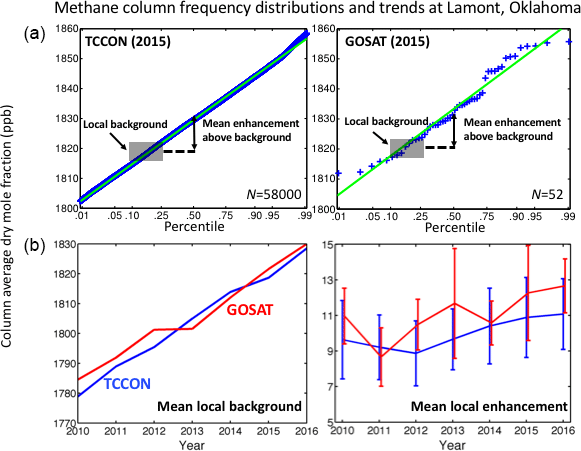
Figure 1Frequency distributions and 2010–2016 trends of methane column average dry mole fractions $X_{{\mathrm{CH}}_{\mathrm{4}}}$ at Lamont, Oklahoma (36.6^∘ N, 97.4^∘ W), as measured by TCCON and GOSAT. The upper panels show the deseasonalized 2015 frequency distributions from TCCON and GOSAT. The percentiles (blue plus signs) are plotted on a normal probability scale such that a normal distribution would plot as a straight line (green). The local background is defined by the 10th–25th percentile range and the mean annual local enhancement relative to this background is defined by the difference with the mean of the distribution. Lower panels compare TCCON and GOSAT backgrounds and enhancements for 2010–2016, with error standard deviations on the enhancements as described in the text.

Download

Here we use the version 7.0 proxy nadir retrievals of GOSAT methane data from Parker et al. (2011, 2015). The proxy method uses prior knowledge of carbon dioxide columns, based on the MACC-II inversion product (v13r2; Chevallier et al., 2010) accounting for seasonal and interannual variations, to infer methane column average dry mole fractions $X_{{\mathrm{CH}}_{\mathrm{4}}}$ (in ppb) from the ratio of retrieved methane and carbon dioxide columns. The proxy method takes advantage of the much larger variability in methane than in carbon dioxide mixing ratios (Frankenberg et al., 2006; Parker et al., 2015). The resulting GOSAT $X_{{\mathrm{CH}}_{\mathrm{4}}}$ data have been validated against the ground-based Total Carbon Column Observing Network (TCCON) and found to be of high quality with a single-scene precision of 0.7 % (random error) and a systematic error of 4–6 ppb (Parker et al., 2015; Buchwitz et al., 2015, 2016). GOSAT observes in all seasons with near-uniform frequency south of 45^∘ N (CONUS and Mexico), but observations further north (Canada) are biased toward summer. The number of successful retrievals over Canada is 2–3 times less in winter than in summer (see Supplement).

From a simple mass balance perspective, enhancements of column methane above the surrounding background in a strong source region can be linearly related to the emissions in that region (Jacob et al., 2016; Buchwitz et al., 2017). Turner et al. (2016) estimated the CONUS background by using glint mode retrievals from GOSAT over the Pacific Ocean for the corresponding latitudes. Bruhwiler et al. (2017) pointed out that changes in large-scale meridional transport could alias trends in this background estimate onto trends in the emissions.

Here we define local background methane for a given CONUS location ($\mathrm{0.5}{}^{\circ }\times \mathrm{0.5}{}^{\circ }$ grid cell, typically including a single repeated GOSAT measurement location) and for a given year as the low (10th–25th) percentiles of the deseasonalized GOSAT methane observations within the given $\mathrm{0.5}{}^{\circ }\times \mathrm{0.5}{}^{\circ }$ grid cell, with seasonality removed using the seasonal-trend-loess (STL) decomposition method (Cleveland et al., 1990). This approach assumes that the low percentiles of concentrations reflect meteorological conditions where local sources have relatively little effect on methane concentrations due to rapid ventilation. Low percentiles are a standard approach for estimating the regional background at a measurement location (Goldstein et al., 1995). By choosing the 10th–25th percentile rather than a lower extreme we guard against the effect of measurement noise (random error). A permutation resampling test shows that GOSAT observations across North America are sufficiently precise that observations ≥10th percentile are not affected by measurement noise (see Supplement). We use the range defined by the 10th–25th percentile range as a measure of uncertainty in the background for the purpose of determining the enhancement.

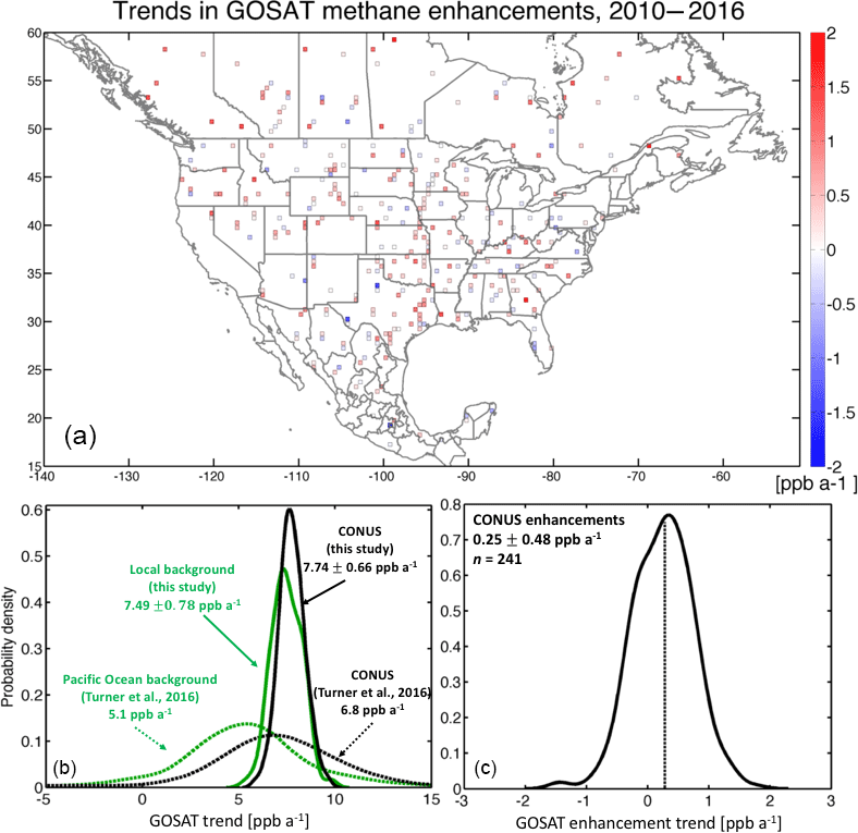
Figure 2The 2010–2016 trends in GOSAT methane enhancements over North America. (a) Ordinary least-squares linear regression trends for $\mathrm{0.5}{}^{\circ }\times \mathrm{0.5}{}^{\circ }$ grid cells with sufficient GOSAT observations, where the deseasonalized annual mean methane enhancements are defined relative to a local low-percentile background as described in the text. The trends are not statistically significant at that resolution (see text). (b, c) Spatial frequency distributions for the $\mathrm{0.5}{}^{\circ }\times \mathrm{0.5}{}^{\circ }$ grid cells over the contiguous United States (CONUS) of mean methane and local background (b), and local methane enhancements computed by difference (c). The dashed black line in the lower-right panel indicates the mean trend in CONUS enhancements. Also shown in the lower-left panel are the 2010–2013 trend distributions from Turner et al. (2016).

Download

Systematic errors of 4–6 ppb in GOSAT observations (Buchwitz et al., 2016) do not affect the enhancement because the bias can be expected to similarly affect all percentiles of the methane observations. Local enhancements are inversely proportional to wind speed (Jacob et al., 2016), but we find no significant trends in wind speeds over the 2010–2016 period that would contribute to our aggregated trends in methane enhancements (see Supplement). Any trends in OH concentrations would also not affect the enhancement because the lifetime of methane against oxidation is 9–10 years (Prather et al., 2012; Kirschke et al., 2013), which is very long compared to the timescale for ventilation from the source region.

We examined the validity of our approach by comparing frequency distributions of GOSAT methane columns and related trends to continuous ground-based column observations available from the TCCON (Wunch et al., 2011) network site at Lamont, Oklahoma (36.6^∘ N, 97.4^∘ W). Figure 1 shows the frequency distributions of the deseasonalized GOSAT and TCCON observations at Lamont. The GOSAT background defined by the 10th–25th percentiles is consistent with TCCON; we see that the repeated observation strategy of GOSAT at its discrete sampling locations makes for a sufficiently dense data set for defining the 10th–25th percentiles with little effect from instrument noise. The local annual mean background increases between 2010 and 2016 in a consistent way in the GOSAT and TCCON data sets, reflecting the global increase in the methane background. The enhancements above background also show comparable 2010–2016 trends between the two data sets, although the error standard deviations defined by the ranges of the 10th–25th percentiles are large and the trends at this single site are marginally significant (p=0.07). Below we will use enhancement statistics aggregated over a large number of sites in order to reduce that uncertainty and quantify trends.

To aggregate trends in methane enhancements for individual source sectors, we use bottom-up annual mean sectoral information with $\mathrm{0.1}{}^{\circ }\times \mathrm{0.1}{}^{\circ }$ spatial resolution from the gridded 2012 US EPA inventory of Maasakkers et al. (2016), the 2013 Canadian and 2010 Mexican oil–gas emission inventories of Sheng et al. (2017), and the EDGAR v4.2 global inventory for 2008 (European Commission, 2011) for other Canadian and Mexican sources. Compared to EDGAR v4.2, the more recent EDGAR v4.3.2 (Janssens-Maenhout et al., 2017) has similar national totals and spatial patterns for non-oil–gas anthropogenic methane emissions in North America. For wetlands, we use multiyear annual mean values from two climatological inventories with $\mathrm{0.5}{}^{\circ }\times \mathrm{0.5}{}^{\circ }$ spatial resolution: (1) the mean of inventories contributing to the Wetland CH₄ Intercomparison of Models Project (WETCHIMP) (Melton et al., 2013) and (2) the 2010–2015 mean of the WetCHARTs extended ensemble wetland methane emissions inventory by Bloom et al. (2017). From these inventories we select high-emitting grid cells at $\mathrm{0.5}{}^{\circ }\times \mathrm{0.5}{}^{\circ }$ resolution dominated by a particular source sector. The high-emitting grid cells are defined as having emissions larger than 0.5 t h⁻¹, encompassing 80 %–90 % of anthropogenic and wetland emissions in all three countries. A high-emitting grid cell is identified as dominated by a given source sector if that source sector accounts for more than 70 % of the total emissions in the cell. This allows us to define grid cells dominated specifically by oil–gas, livestock, waste, and wetland emissions. Contributions from other sectors (up to 30 %) may lead to some smoothing of results. Wetland-dominated areas determined by the WETCHIMP mean and WetCHARTs inventories differ significantly (see Supplement). Using either of the two inventories alone may bias our results, and thus we conservatively require wetland-dominated areas to be determined as such in both inventories.

Figure 3Methane emissions in North America and contributions from different source sectors. (a) shows $\mathrm{0.5}{}^{\circ }\times \mathrm{0.5}{}^{\circ }$ grid cells with high emissions dominated by a particular sector as identified by the bottom-up inventories (see text for details). High-emitting wetland areas are those identified by both the WETCHIMP mean inventory and the Bloom et al. (2017) mean inventory. Livestock includes enteric fermentation and manure management. Oil/gas includes the complete systems from production to distribution. Waste includes landfills and wastewater plants. (b) shows national emissions for 2008–2013 from the bottom-up inventories. “Other” includes smaller sources from coal, rice, combustion, petrochemical production, ferroalloy production, and biomass burning. Total emissions in the high-emitting wetland areas are indicated by gridded areas.

Download

We define a total methane enhancement Δ for a given year, source sector, and country as

where ${\overline{X}}_{{\mathrm{CH}}_{\mathrm{4}},i}$ is the annual mean value of the deseasonalized column average dry mole fractions in the $\mathrm{0.5}{}^{\circ }\times \mathrm{0.5}{}^{\circ }$ grid cell i for the given year, $X_{{\mathrm{CH}}_{\mathrm{4}},\mathrm{b},i}$ is the corresponding local background value, and the summation is over all high-emitting grid cells for that sector and country. We require grid cells to have at least eight valid retrievals for a given year (to avoid bias in the annual mean value and percentiles), and about 70 % of grid cells meet this requirement. To account for local background variation due to atmospheric transport, the summation in Eq. (1) is conducted for 1000 Monte Carlo realizations where the background $X_{{\mathrm{CH}}_{\mathrm{4}},\mathrm{b},i}$ for each grid cell and for individual years is obtained by random sampling of percentiles in the 10th–25th range. Results are only weakly sensitive to the choice of that range (see Supplement). The resulting summation statistics define the probability density function of the total enhancement Δ, and this is used in what follows to test the statistical significance of year-to-year trends in Δ.

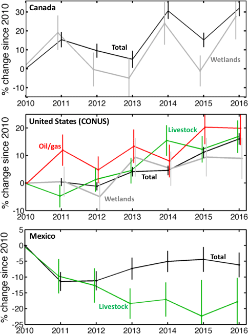
Figure 4National trends in methane emissions since 2010 inferred from GOSAT, and contributions from specific source sectors where sufficient data are available. The trends are defined by relative year-to-year changes in the summed methane enhancements Δ relative to the local backgrounds as computed from Eq. (1), and vertical bars are standard deviations derived from uncertainty in the local background (see text).

Download

Figure 2 (upper panel) shows the spatial distribution of GOSAT methane trends in local enhancements over North America at $\mathrm{0.5}{}^{\circ }\times \mathrm{0.5}{}^{\circ }$ spatial resolution from January 2010 to December 2016 (7 years of data). The $\mathrm{0.5}{}^{\circ }\times \mathrm{0.5}{}^{\circ }$ trends are inferred from ordinary least-squares linear regression of the enhancements for individual years. The trends are not statistically significant at that resolution. We will aggregate grid cells in what follows to increase statistical significance. Some areas are sparsely sampled, such as California, while the central US is more densely observed due to a more regular schedule of standard measurements. This sampling bias in California is unlikely to affect the trend estimate on the national scale because California accounts for less than 5 % of the US national total according to the bottom-up inventories. Spatial averaging to $\mathrm{4}{}^{\circ }\times \mathrm{4}{}^{\circ }$ as in Turner et al. (2016) does not improve significance (see Supplement) because methane emissions are not correlated on that scale. A major reason for the weaker statistical significance of our results relative to Turner et al. (2016) is the choice of background. Enhancements defined relative to the Pacific background, as in Turner et al. (2016), are larger than in our approach where the background is defined locally.

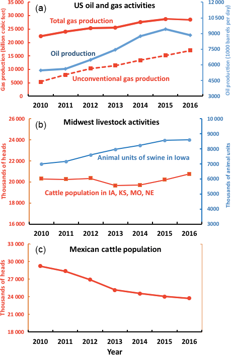
Figure 5The 2010–2016 changes in methane-emitting activities. (a) Oil and natural gas production in CONUS (Drillinginfo, 2016). (b) Cattle population in Iowa, Kansas, Missouri, and Nebraska (USDA National Agricultural Statistics Service, 2015a), and animal units of swine in Iowa (Iowa Department of Natural Resources, 2017). One animal unit accounts for 3–5 heads of swine depending on body weight(USDA National Agricultural Statistics Service, 1995). (c) Total cattle population in Mexico (USDA Foreign Agricultural Service, 2015).

Download

We improve the statistical significance of the CONUS enhancement trends by taking national statistics over all $\mathrm{0.5}{}^{\circ }\times \mathrm{0.5}{}^{\circ }$ grid cells. This is shown in the lower panels of Fig. 2 with the CONUS frequency distribution of trends in mean methane, local background, and the enhancements computed by difference. The mean 2010–2016 trend in methane enhancements over CONUS is 0.25±0.48 ppb a⁻¹ (mean ± 1 standard deviation), which is statistically significant (sample size n=241 and p value < 0.01). The mean 2010 methane enhancement for high-emitting grid cells in CONUS relative to local background is 10.8 ppb, which is comparable to that found by Janardanan et al. (2017). If this mean enhancement is taken as a measure of CONUS emissions, then a 0.25±0.48 ppb a⁻¹ trend implies a 2.3±4 % a⁻¹ increase in emissions for 2010–2016. The Turner et al. (2016) frequency distributions, shown in the lower-left panel, are much broader than ours because they did not use annual averaging of the data. Their Pacific background distribution is similarly broader and is also lower than our local background, which is appropriately elevated by continental influences. Below we will use the aggregated enhancements by source sectors (Eq. 1) to infer the trends and reduce the uncertainty.

Figure 3 shows the locations of high-emitting $\mathrm{0.5}{}^{\circ }\times \mathrm{0.5}{}^{\circ }$ grid cells dominated by different sectors as identified by the bottom-up inventories of Sect. 2. Also shown are national emission totals from these inventories. Wetland-dominated areas in Fig. 3 are those identified by both the WETCHIMP mean and Bloom et al. (2017) inventories in order to avoid false positives. There is clear separation of grid cells dominated by wetlands, oil–gas, and livestock source sectors. Waste emissions dominate in urban areas but are more localized. Offshore oil–gas emissions over the Gulf of Mexico account for more than 50 % of Mexican oil–gas total (Sheng et al., 2017), but are not directly detectable by GOSAT nadir measurements over land. Glint observations are available over the ocean but are much sparser.

Figure 4 shows GOSAT methane enhancement trends for 2010–2016 (expressed as percent change since 2010) over Canada, CONUS, and Mexico, along with contributions from the sector-resolved high-emitting grid cells. Here the trends are calculated for the summed enhancement Δ in Eq. (1) calculated for individual years and for high-emitting grid cells of individual countries or high-emitting sectors. Inferring significant trends for a given source sector generally requires ∼50 contributing $\mathrm{0.5}{}^{\circ }\times \mathrm{0.5}{}^{\circ }$ grid cells. The largest source of uncertainty is the selection of the local background within the 10th–25th percentile range, and this is reflected by the error bars in the figure.

The Canadian methane emissions show no significant 7-year trend but large year-to-year variability driven by wetlands. The 2014 maximum can be explained by a maximum of wetland areal extent (Bloom et al., 2017) (see Fig. S6 in Supplement). Observations in the oil–gas-dominated region of Canada (mainly natural gas in Alberta) are too sparse for inferring a significant oil–gas emission trend and are not shown here.

Mexican national emissions (excluding oil–gas offshore emissions) show a 5 %–10 % decrease over the 2010 to 2016 period that appears to be largely driven by livestock. The decrease in livestock emissions (4.0±1.6 % a⁻¹) is consistent with the 17 % decrease in the Mexican cattle population over that period as reported by the Foreign Agriculture Service of the US Department of Agriculture (2015) and shown in Fig. 5. The slight increase in Mexican emissions from 2012 on suggests an increasing source to compensate for the declining livestock emissions but GOSAT observations are too sparse to identify that source.

The CONUS data imply a significant increase in methane emissions from 2010 to 2016, with a trend of 2.5±1.4 % a⁻¹ derived from linear regression that is consistent with our previously calculated mean trend of 2.3 % a⁻¹ averaged over the $\mathrm{0.5}{}^{\circ }\times \mathrm{0.5}{}^{\circ }$ gridded trends in Fig. 2. Breakdown by sector suggests that US oil–gas emissions increased at a marginally significant level (2.9 % a⁻¹, p=0.03) from 2010 to 2016. Oil and unconventional (hydraulic fracturing) gas production grew by 15 % a⁻¹ and 19 % a⁻¹, respectively, during that period (Fig. 5), though production rate is not necessarily a predictor of emissions (Peischl et al., 2015).

The US livestock emissions show a 3.5±1.8 % a⁻¹ increase in our analysis, largely reflecting the agricultural Midwest where high-emitting grid cells are concentrated (Fig. 3). These grid cells emit 0.95 Tg CH₄ a⁻¹ from enteric fermentation (cattle) and 0.55 Tg CH₄ a⁻¹ from manure management (swine) according to the gridded EPA inventory (Maasakkers et al., 2016). The cattle population in that region does not show a significant trend (Fig. 5), but the swine population in Iowa (accounting for most of the swine population in the Midwest) increased by two million heads from 2010 to 2016 (USDA National Agricultural Statistics Service, 2015b; Iowa Department of Natural Resources, 2017) (Fig. 5). This would increase swine manure management emissions by 0.02–0.1 Tg CH₄ a⁻¹ over the 2010–2016 period, assuming the IPCC (2006) emission factor of 10–45 kg CH₄ head⁻¹ a⁻¹. Here a larger value of the emission factor is more likely. The emission factor may have increased during that time due to an increase in swine body weight and a 30 % rise in concentrated animal feeding operations (CAFOs) with more than 1000 animal units (Iowa Department of Natural Resources, 2017). Those CAFOs tend to use liquid manure storage (US EPA, 2016) and have extended manure storage time (Iowa Department of Natural Resources, 2011), which lead to greater methane emissions. A recent bottom-up study from Wolf et al. (2017) found a steady increasing trend since the 1990s in US methane emissions from manure management.

US wetland emissions do not show a significant trend over 2010–2016 but large year-to-year variability, which contributes in part to the total national trend after 2012. Correlation with driving variables in the WetCHARTs yearly ensemble of Bloom et al. (2017) suggests that this year-to-year variability is related to wetland areal extent, same as for Canada (see Fig. S6 in Supplement), though the definition of wetland areal extent may vary significantly (Poulter et al., 2017). Here the WetCHARTs extended ensemble used (i) GlobCover land cover data (Bontemps et al., 2011) and the Global Lakes and Wetlands Database (GLWD; Lehner and Dölla, 2004) to represent spatial wetland extent and (ii) ERA-Interim precipitation to account for temporal wetland extent (Bloom et al., 2017).

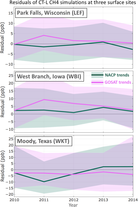
Figure 6Time series of the residuals (observed minus simulated methane concentrations) of the CarbonTracker-Lagrange (CT-L) CH₄ transport model simulations driven by posterior emissions optimized for NACP data (green) and scaled to GOSAT-inferred emission trends (purple) for three surface sites particularly sensitive to emissions from different sectors: LEF (45.9^∘ N, 90.3^∘ W), WBI (41.7^∘ N, 91.4^∘ W), and WKT (31.3^∘ N, 97.3^∘ W). Solid lines show the medians of NACP and GOSAT trends, and shaded areas show the 25th–75th percentile envelope.

Download

Inverse analyses of methane concentrations in surface air measured as part of the North American Carbon Program (Wofsy and Harris, 2002) for 2010–2014 reveal no significant trends in US emissions over that period (Benmergui et al., 2015). We examined whether the trends inferred from this work (significant trends after 2012) are consistent with the information provided by NACP surface data. For this purpose, we examined the residuals (observed minus simulated methane concentrations) of the CarbonTracker-Lagrange (CT-L) methane transport model (Benmergui et al., 2015) driven with two sets of emissions: (1) the CT-L posterior emissions for 2010–2014 that are optimized to match all NACP data and show no significant trend and (2) a scaled version of the CT-L posterior emissions that matches the sector-resolved trends derived in this work. Figure 6 shows annual statistics and trends of the residuals for both simulations at three NACP sites included in the CT-L inversion: LEF (Park Falls, Wisconsin; 45.9^∘ N, 90.3^∘ W), WBI (West Branch, Iowa; 41.7^∘ N, 91.4^∘ W), and WKT (Moody, Texas; 31.3^∘ N, 97.3^∘ W). These sites are strongly influenced by large livestock and/or wetlands, livestock, and oil–gas sources, respectively (Benmergui et al., 2015). There is no significant trend in the residuals of the CT-L simulation driven by either our GOSAT-inferred emission trends or CT-L posterior emissions, and the two sets of residuals are statistically indistinguishable. We find similar results for other NACP sites that are less sensitive to source regions. This implies that the trends found in this work are compatible with the constraints provided by NACP data. This also suggests that the surface data may be spatially too sparse to adequately infer trends of the magnitude detected by GOSAT.

The GOSAT Proxy $X_{{\mathrm{CH}}_{\mathrm{4}}}$ data (Parker et al., 2015) used in this publication are available from http://www.esa-ghg-cci.org/sites/default/files/documents/public/documents/GHG-CCI_DATA.html (last access: 1 December 2017). The TCCON $X_{{\mathrm{CH}}_{\mathrm{4}}}$ data (Wunch et al., 2011) used in this publication are from https://tccondata.org/ (lass access: 1 December 2017). The North American Carbon Program (NACP) data (Wofsy and Harris, 2002) used in this publication are from https://www.nacarbon.org/ (last access: 1 December 2017).

The supplement related to this article is available online at: https://doi.org/10.5194/acp-18-12257-2018-supplement.

JXS and DJJ designed the research; JXS and DJJ performed the research; JXS analyzed the GOSAT data; JDM and AAB provided the bottom-up CH₄ emission inventories; JB performed CarbonTracker-Lagrange model simulations; HB and RJP provided the GOSAT data; JXS and DJJ wrote the paper; all the authors discussed the results and contributed to the manuscript.

The authors declare that they have no conflict of interest.