2.1 MIPAS

2.2 Aerosol in situ measurements from Laramie, Wyoming

To validate the new MIPAS aerosol data set described in Sect. 3, we use aerosol volume density profiles that were derived from in situ measurements of stratospheric aerosol above Laramie, Wyoming (41^∘ N, 105^∘ W) (Deshler et al., 2003). Size-resolved aerosol concentration measurements from the surface to approximately 30 km altitude were made with balloon-borne optical aerosol counters, which were developed and operated by the University of Wyoming. Measurements usually occurred between 06:00 and 09:00 LT, with measurement frequency varying from monthly to bimonthly. Data are available from 1971 to present. Over this time period, three different primary instrument types were used. The most recent type (laser particle counters, LPCs) of the three instrument types was used first in 2006, became the standard Laramie instrument in 2008, and was, as an example, also flown on quasi-Lagrangian balloons in Antarctica in 2010 (Ward et al., 2014). While the transition from the first instrument to the second was documented in Deshler et al. (2003), a similar study comparing the third Wyoming instrument with the second instrument is a work in progress. For the MIPAS validation, measurements from the second and third Wyoming instruments were available. The positive bias of MIPAS aerosol volumes from the in situ measurements was generally consistent between MIPAS and both of the Wyoming instruments above 20 km. Below 20 km the in situ measurements diverged from each other, with the second instrument indicating higher volumes than the LPC (third instrument) and at times higher volumes than MIPAS. Based on these comparisons with both instruments the Wyoming measurements to be used were confined to those made with the LPC because it permitted the simplest altitude-dependent de-biasing function for the MIPAS aerosol volume densities. The LPC measures particles with radii > 0.08–4.2 µm in eight size classes. Deriving geophysical quantities from the size-resolved aerosol concentration measurements requires fitting a size distribution to the in situ data. In the past this was done by fitting either a unimodal or bimodal lognormal size distribution to a subset of the measurements. The final size distribution parameters selected are those from that subset of the measurements which minimises the root mean square error when the fitted distribution is compared to all the measurements. This approach is transitioning to a new approach which modifies the nominal in situ aerosol sizes based on laboratory measurements of the aerosol counting efficiency. The counting efficiency at each size is then included in a search of the lognormal parameter space for the lognormal coefficients which minimise the error of the fitted distribution, coupled with the counting efficiency, compared to the measurements. In our study we use the volume density profiles that are derived from the fitted lognormal size distributions (unimodal or bimodal, following the new retrieval approach) of the measurements. The precision of these volume estimates is the same as the old method, ±40 % (Deshler et al., 2003). The change in the method with which the fitting parameters are derived is the subject of a paper to be submitted soon. The impact on size distributions from the LPC measurements is not large.

2.3 Chemical transport model

The chemical transport model (CTM) used in our study (e.g. Sinnhuber et al., 2003; Kiesewetter et al., 2010) is forced by temperature, wind fields, and diabatic heating rates from ERA-Interim (Dee et al., 2011). The model uses isentropes as vertical coordinates. Horizontal transport at levels of constant potential temperature is derived from the wind fields, while vertical transport is calculated using the diabatic heating rates. The CTM employs the second-order moments advection scheme by Prather (1986). The model domain covers 29 isentropic levels between 330 and 2700 K (∼ 10–55 km), with a horizontal resolution of about 2.5^∘ latitude × 3.75^∘ longitude (Gaussian latitude grid).

As part of this study, a sulfur module has been implemented, including OCS, SO₂, and H₂SO₄ as advected tracers. In the sulfur module no distinction between tropospheric and stratospheric air is implemented. In the presented simulations, we consider volcanic SO₂ from one volcanic eruption as the only sulfur source per simulation, in order to study the SO₂ and sulfate aerosol after the eruptions of Kasatochi in 2008 and Sarychev in 2009 individually. Therefore, OCS is not considered as a sulfur source in the simulations presented in this work. The bottom boundary concentrations and initial fields are set to zero for SO₂ and H₂SO₄. The volcanic SO₂ is injected instantaneously into the model column of the volcano. SO₂ masses are injected into three altitude ranges (see Sect. 4.1, Table 1), consistent with MIPAS SO₂ observations, and SO₂ is uniformly distributed to the air mass within each altitude range. The sulfur released from volcanic SO₂ reacts with OH (hydroxyl radical) to form H₂SO₄. This is the only chemical reaction considered in the simulations presented in this study. As the interim product sulfur trioxide (SO₃), formed during the oxidation of SO₂, combines rapidly with water vapour to form sulfuric acid, it is not explicitly considered in the model. The removal processes of the species are advective transport out of the model domain into the troposphere, the decay of SO₂ by its reaction with OH, and the gravitational settling of sulfate aerosol. An OH climatology of daily distributions was derived in a full chemistry run of the CTM (2003–2006), and for reaction rates the recommendations from JPL (Jet Propulsion Laboratory) are used (Burkholder et al., 2015). For the sedimentation of sulfate aerosol, equilibrium partitioning between the gas and the liquid phase is assumed for H₂SO₄ (Ayers et al., 1980) at each simulation time step. To determine the terminal velocity for the part of the sulfate aerosol that settles, velocity calculations follow the approach suggested by Jacobson (1999). In the simulations presented here, the aerosol radius is fixed to one effective settling radius. The solution density of the aerosol is calculated online from the fraction of liquid-phase H₂SO₄ in the binary solution of the H₂SO₄–H₂O aerosol. The sulfur scheme hydrates the sulfate aerosol based on ambient water vapour loading, which is assumed to be 4.5 ppmv. Sedimentation transports sulfate aerosol into the grid box below or finally out of the model domain. All model results shown for H₂SO₄ only consist of the sulfate aerosol droplets, as the MIPAS measurements do not consider gas-phase H₂SO₄.

The model is run for 365 d per simulation, with a time step of 30 min and tracer fields are written out daily at 12:00 UTC. For the eruption of Kasatochi (7 August 2008) the individual runs are started on the 31 July 2008, and for the eruption of Sarychev (12 June 2009) all runs are started on the 31 May 2009. As the relevant initial trace gas fields are set to zero and the model is driven by ERA-Interim data, which are updated every 6 h, no long spin-up time is needed. Per volcano four simulations were made that differ concerning the particle size of sulfate aerosol. Simulations were made with constant radii of 0.1, 0.5, and 1 µm, and without sedimentation. In the atmosphere the radius of sulfate aerosol varies (Deshler et al., 2003; Deshler, 2008). Nevertheless, for simplification, we use a constant “effective sedimentation radius” to determine the terminal fall velocity, which we consider to be the average settling speed of aerosol particles of different radii. In our simple sulfur scheme, no scavenging of SO₂ or H₂SO₄ by clouds is considered in the model. This would be confined mostly to tropospheric altitudes and in our study region (≥ 10 km) especially to tropical latitudes. Washout by precipitation might play a role there, but it is expected to have a minor effect on our study, as we analyse the sulfur that remains in the atmosphere (above ∼ 10 km) after the first weeks following the volcanic eruptions. Furthermore, no nucleation or growth processes of sulfate aerosol are considered.

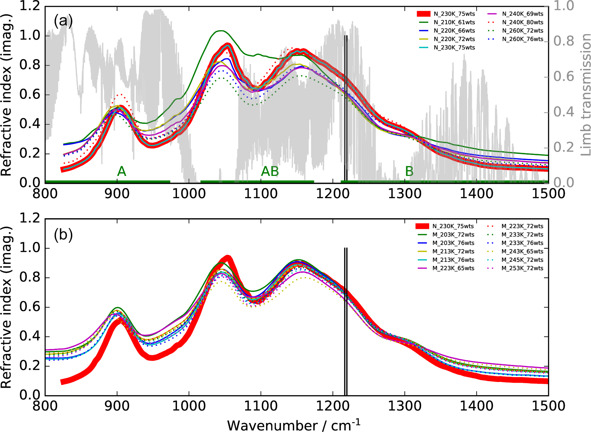
Figure 1Imaginary parts of refractive indices for aqueous H₂SO₄ solutions of different concentrations (wts: weight % H₂SO₄) and different temperatures in the mid-infrared region. (a) Thin solid and dotted curves: Niedziela et al. (1999); (b) Lund Myhre et al. (2003). The bold red line indicates the data set, and the two vertical lines the spectral window used in this study. A simulated limb transmission spectrum for 10 km tangent altitude for standard midlatitude conditions is additionally plotted in the top row as are the wavenumbers covered by MIPAS bands A, AB, and B.

Download

3.1 Aerosol retrieval from MIPAS limb-spectra

In previous analyses of mid-infrared observations by MIPAS-B (the balloon-borne predecessor of the MIPAS satellite instrument; Friedl-Vallon et al., 2004) and MIPAS/Envisat (MIPAS instrument on the satellite Envisat, generally referred to as “MIPAS” throughout the present work), it has been demonstrated that the limb radiances due to particles have two major contributing terms: (1) the thermal emission of the particles and (2) the scattered radiation from the atmosphere and Earth's surface from below the tangent point (Höpfner et al., 2002, 2006). The relative weights of these contributions differ with particle size and wavenumber. For particles sufficiently small compared to the wavelength (d < ∼ 1 µm in the mid-IR; Höpfner, 2004), the scattered contribution can be neglected such that only the thermal emission remains as major source of IR radiation. In this wavenumber length regime, the radiance only depends on the total aerosol volume density. Typical sizes of the stratospheric aerosol layer particles are less than 1 µm in the case of background and enhanced conditions due to medium-sized volcanic eruptions (e.g. Deshler et al., 2003). Thus, our retrieval target is the altitude profile of volume densities, derived from each set of calibrated MIPAS limb-scan spectra.

For this study we have concentrated on the second MIPAS measurement period between January 2005 and April 2012. The retrieval model used is the KOPRA–KOPRAFIT (Karlsruhe Optimized and Precise Radiative transfer Algorithm) suite, allowing us to directly retrieve aerosol parameters from observed radiances by coupling a Mie model with the line-by-line radiative transfer scheme (Stiller et al., 2002; Höpfner et al., 2002, 2006). For aerosol composition we assume a 75 % by weight (75 wt %) H₂SO₄–H₂O solution, as the stratospheric sulfuric aerosol composition typically varies between around 70 and 80 %, as obtained by equilibrium calculations (Carslaw et al., 1995) and observations (e.g. Doeringer et al., 2012). Kleinschmitt et al. (2017), calculating aerosol optical properties, Kremser et al. (2016), calculating sulfur fluxes, and Gao et al. (2007), calculating atmospheric volcanic aerosol loadings, also use a 75 wt % H₂SO₄–H₂O composition in their studies. The imaginary parts of various refractive index data sets in the mid-IR are displayed in Fig. 1. Here the optical constants used in our study, which are based on Niedziela et al. (1999) for 75 wt % and 230 K (bold red line), are compared to data at other concentrations and temperatures, based on optical constants given by Niedziela et al. (1999) (Fig. 1a) and Lund Myhre et al. (2003) (Fig. 1b). This particular data set has been chosen because in an evaluation of optical constants for sulfuric acid, Wagner et al. (2003) found these data sets to be best consistent with observations in the aerosol chamber AIDA (Aerosol Interactions and Dynamics in the Atmosphere). The spectral range selected for the retrieval (1216.5–1219.5 cm⁻¹) is situated at the long wavelength end of MIPAS band B as indicated by the two vertical lines in Fig. 1. It lies within one of the atmospheric windows as can be seen by comparison to the limb-transmission curve (light grey) in Fig. 1. We have not chosen the windows at around 830 and 950 cm⁻¹ since at 1220 cm⁻¹ the absorption by H₂SO₄ droplets is higher and the relative difference between the various sets of refractive indices is smaller.

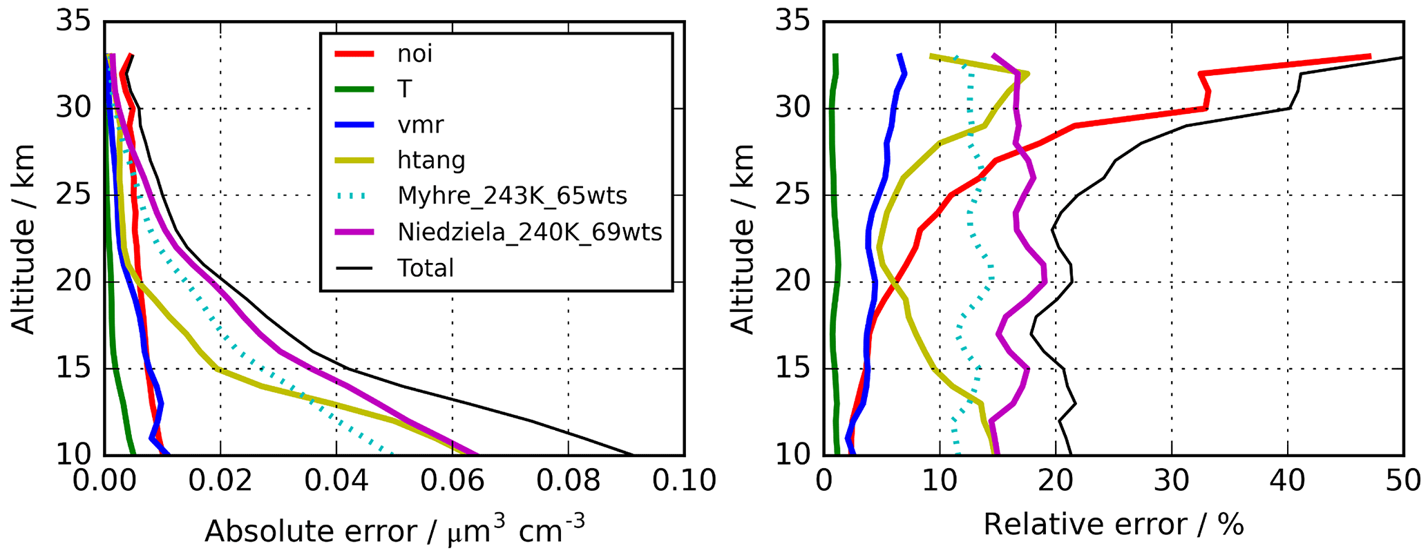
Figure 2Altitude-dependent estimated errors for the retrieval of H₂SO₄–H₂O aerosol volume densities. Solid lines indicate the uncertainties used to calculate the “total” error. Indicated errors are “noi” – single scan spectral noise; “T” – temperature uncertainty 2 K; “vmr” – 10 % uncertainty in volume mixing ratios of interfering gases; “htang” – 300 m tangent altitude uncertainty; “Niedziela_240K_60wts” – use of optical constants by Niedziela et al. (1999) for 240 K and 69 wt % instead of Niedziela et al. (1999) for 230 K and 75 wt % H₂SO₄. The dotted curves (“Myhre_243K_65wts”) show the results when the optical constants of Lund Myhre et al. (2003) for a temperature of 243 K and a concentration of 65 wt % are used instead of those by Niedziela et al. (1999) (T=230 K and 75 wt %).

Download

The retrieval has been set up as a multiparameter nonlinear least-squares fit of the calculated to the measured limb radiances of entire limb scans (e.g. von Clarmann et al., 2003). Besides the target parameter, namely sulfate aerosol volume densities, further atmospheric fit parameters of the retrieval are the vertical profiles of spectrally interfering trace gases methane (CH₄), H₂O, ozone (O₃), and nitric acid (HNO₃). While zero initial guess profiles have been used for the aerosol volume densities, results from the IMK routine processing are taken for the trace gases (von Clarmann et al., 2009). As the atmospheric parameters are represented at denser altitude levels (1 km) than the vertical field of view (∼ 3 km) and the vertical tangent point spacing (1.5 km) of MIPAS, constraints on the smoothness of the profile shape are introduced by regularisation (Tikhonov, 1963; Steck, 2002). The retrieval of aerosol volume density is restricted to altitudes of up to 33 km, and the regularisation strength has been adjusted such that its resulting vertical resolution is around 3 to 4 km. To cover instrumental uncertainties, a spectral shift parameter and a radiance offset, constant over all wavenumbers and tangent altitudes, have been retrieved simultaneously with the atmospheric quantities. For the analysis in this paper, only data at altitudes with averaging kernel diagonal elements larger than 0.05, which refer to altitudes at least 1 km above the lowest tangent height, are used.

An overview of the leading error components is presented in Fig. 2, with the assumed parameter uncertainties listed in the caption. The error contributions are estimated from a subset of a few hundred single cases by sensitivity studies using perturbed parameters or, in the case of spectral noise, directly from the retrieval diagnostics. The total error changes with altitude from around 20 % (0.09 µm³ cm⁻³) at 10 km up to over 40 % (0.005 µm³ cm⁻³) at 30 km. It is dominated by the uncertainty in the optical constants resulting in 10–20 % error, followed by tangent pointing knowledge with 5–15 %. The error component resulting from spectral noise is fairly constant with altitude in absolute terms of volume density and amounts to about 0.01 µm³ cm⁻³. Other instrumental errors that have been investigated but are not listed in Fig. 2 are uncertainties due to the knowledge of the instrumental line shape and radiometric gain and offset calibration error. In the estimation of the radiative error, no radiometric offset variation with tangent altitude was considered, and, thus, it was not compensated for by the retrieval approach. However, a tangent altitude-dependent radiometric offset error caused, e.g. by stray light in the instrument cannot be excluded (López-Puertas et al., 2009). We have not handled this uncertainty in the framework of error estimation, but we have tried instead to compensate for it through a de-biasing of the data set based on validation with in situ observations as described in Sect. 3.2.

Prior to the retrieval, a deselection of spectra affected by clouds was performed via the application of an established cloud filter method for MIPAS by Spang et al. (2004). To sort out optically thick clouds, but not all aerosol-affected spectra, this cloud filter was applied with a cloud index limit of 1.7. Due to this loose setting of the cloud-filter, artefacts caused, e.g. by thin cirrus clouds, polar stratospheric clouds (PSCs), or volcanic ash remain in the data set and are all attributed to the retrieved 75 wt % H₂SO₄–H₂O aerosol volume density. Thus, further filtering of affected profiles was necessary after completing the retrieval.

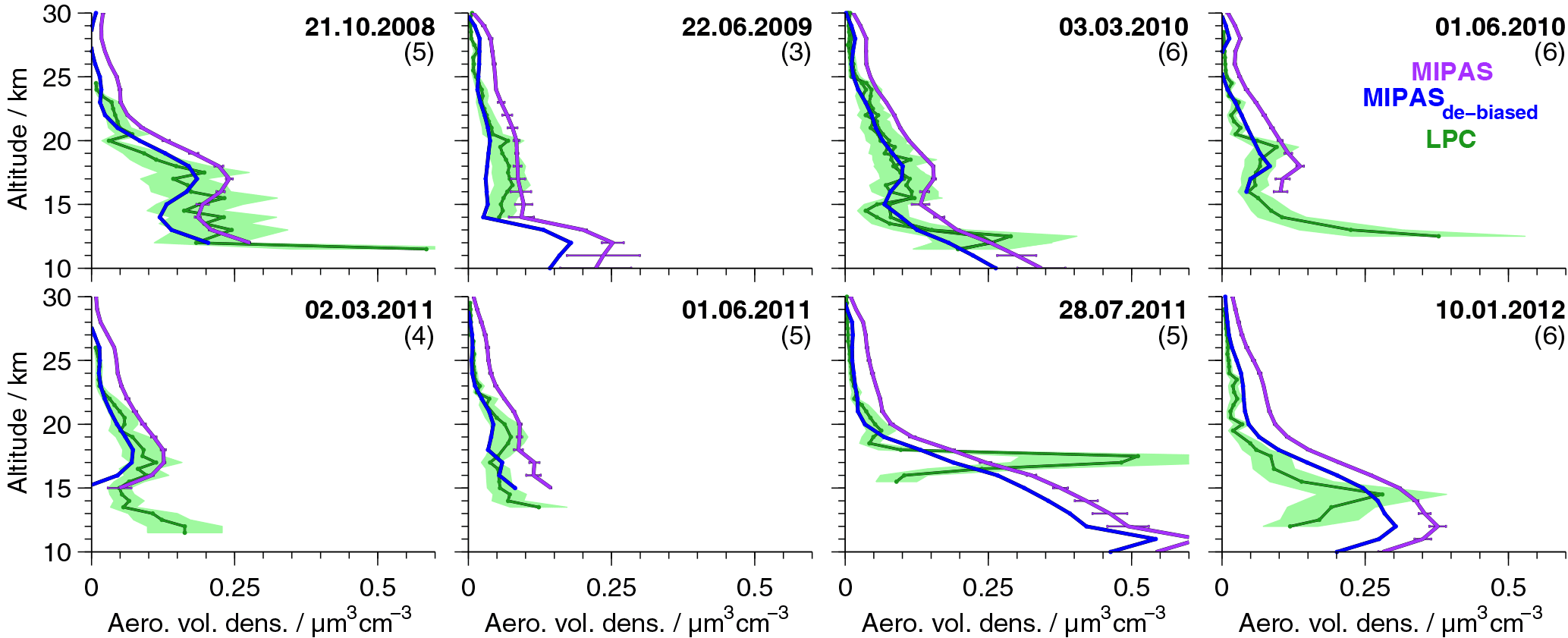
Figure 3Profiles of aerosol volume densities from in situ and MIPAS satellite measurements. In situ data are balloon-borne data above the lapse rate tropopause for Laramie, Wyoming (41^∘ N, 105^∘ W), measured by laser particle counters. Two instruments were flown on the 3 March 2010. The 40 % errors of the in situ data are shown as green shaded areas. MIPAS satellite data are shown in purple (original data) and blue (de-biased data). On all MIPAS data the ice filter by Griessbach et al. (2016) and ash filter by Griessbach et al. (2014) and our PSC filter have been applied. MIPAS profiles are averages of all available profiles for the indicated day, averaged in a ±5^∘ lat × 10^∘ long area. The number of MIPAS profiles included in the average is given in brackets. The 1σ standard errors of the mean profiles are shown for the non-de-biased MIPAS values.

Download

Two distinct features of strong enhancements with an annual cycle show up in the unfiltered data set. The first feature is due to strong enhancements in the presence of PSCs at the winter pole. To deselect PSC-affected profiles, a filter is applied when temperatures in the altitude range 17–23 km drop below a threshold of 195 K polewards of 40^∘ for the Northern Hemisphere from 15 November to 15 April and for the Southern Hemisphere from 1 April to 30 November. This temperature represents the nitric acid trihydrate (NAT) existence temperature at around 20 km under typical stratospheric conditions for nitric acid and water vapour.

The second feature is assumed to be induced by thin cirrus clouds. It is present mainly in the tropics, at around 25^∘ S–25^∘ N, at altitudes between about 13 and 21 km. It reaches the highest altitudes and is most intense above and in the vicinity of continents and above the western Pacific. The vertical extent is smallest in boreal summer, and its vertical gradient towards lower aerosol volume densities is relatively strong, with no upward transport being observed. Both the location in the tropics, in regions of strong vertical motions and convective clouds, and the relatively sharp decrease at higher altitudes towards increasing temperatures suggest that it is connected to the influence of ice particles. The ice filter for MIPAS data by Griessbach et al. (2016) is applied to all retrieved MIPAS aerosol profiles to reduce the effect of spectra influenced by ice in the present data set. Their method consists of two steps to detect whether MIPAS spectra are influenced by aerosols, ice, clouds, ashes, or a clear sky (Griessbach et al., 2014, 2016). First, aerosols and clouds are identified, using a spectral window region that is sensitive to aerosols and clouds. Then ice clouds and aerosols are distinguished, using information from spectral windows with contrasting behaviour for ice and aerosols. In our data set, we consider only retrieved values starting 4 km above the altitude of the uppermost spectrum that was flagged to have been influenced by ice. Further, the ash filter for MIPAS spectra by Griessbach et al. (2014), based on an ash detection threshold function, is applied in the same way as the ice filter, to filter out volcanic ash and mineral dust.

3.2 Validation and bias correction

To validate the new data set, we compare the profiles of MIPAS aerosol volume density to in situ balloon measurements (Deshler et al., 2003). In situ measurements were carried out with laser-based aerosol spectrometers from Laramie, Wyoming (41^∘ N, 105^∘ W), between 06:00 and 09:00 LT. In Fig. 3, profiles of the balloon measurements are shown. In comparison, MIPAS mean aerosol volume density profiles are presented, selected from a restricted area around Laramie, together with their standard errors (Fig. 3), which show the variability in the underlying profiles. MIPAS profiles are chosen for the day of the balloon flight within a 5^∘ latitude × 10^∘ longitude distance around Laramie. Further, in Fig. 4a we show the mean over the profiles that were retrieved from LPC measurements, as shown in Fig. 3 (excluding the 28 July 2011) and the corresponding MIPAS profiles, together with the absolute (panel b) and relative difference (panel c) of the mean MIPAS profile to the mean profile from balloon measurements. In Fig. 4a the measurement uncertainties of the mean profiles are presented, and in Fig. 4b the uncertainty in the bias (difference between the mean in situ and mean MIPAS profile) is shown. The profile on the 28 July 2011 shows large differences between MIPAS and the in situ data and the strongest vertical variability in all in situ profiles at low altitudes (below ∼ 18 km), possibly due to the Nabro eruption (12 June 2011). Hence, this profile is excluded from the calculation of the mean profiles shown in Fig. 4.

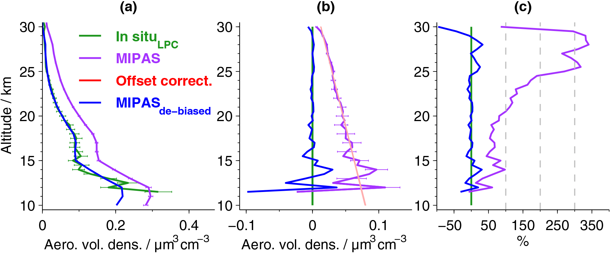
Figure 4Aerosol volume densities by MIPAS and in situ data from Laramie, Wyoming. (a) Mean profiles for data in Fig. 3 (excluding the 28 July 2011), and their 1σ errors, based on the estimated measurement uncertainties. De-biased MIPAS values are shown in blue; the original data are shown in purple. (b) Absolute and (c) relative differences of MIPAS to LPC in situ data. Differences are calculated for the mean profiles shown in (a). In (b) the uncertainties of the absolute differences between in situ and MIPAS data are shown (horizontal purple lines; error propagation based on MIPAS and in situ errors presented in a). Red line: linear fit to the profile of absolute differences (purple line) between 18 and 30 km, used to reduce the bias to the LPC in situ measurements (light red area: 1σ uncertainty in the linear fit).

Download

Generally, the aerosol volume densities (Figs. 3 and 4) are highest in the lower stratosphere and then decrease towards zero at higher altitudes. As the balloon data have a higher vertical resolution and the retrieval process for MIPAS profiles includes smoothing, the in situ data show finer structures. Compared to the balloon data, the original MIPAS aerosol volume densities show a positive bias in most profiles (Fig. 3) as well as in the mean profile (Fig. 4). This is most easily detectable at higher altitudes where profiles are relatively smooth. The offset amplifies towards lower altitudes (Fig. 4b). Aiming at a reduction in this positive offset, a height-dependent de-biasing is performed on all single MIPAS profiles. The de-biasing is based on the in situ measurements carried out with laser-based particle counters. MIPAS profiles show a consistent variation with height, compared to the LPC measurements. An additive linear de-biasing is applied, rather than a multiplicative correction, as the offset is expected to be caused by an altitude-dependent additive stray light error in the radiances (see Sect. 3.1). The de-biasing is based on the absolute differences between the aerosol volume densities of the mean MIPAS and in situ profiles (Fig. 4b, purple solid profile) at 18–30 km, where profiles show weak variability and a relatively low uncertainty in the bias. A regression line (Fig. 4b, red line) to the profile of absolute differences represents the vertically resolved values of the de-biasing function, which are subtracted from each MIPAS profile during offset correction. A narrow red shaded area indicates the uncertainty in the bias correction and has been evaluated using generalised Gaussian error propagation of the uncertainties of the slope and the intercept of the regression line. No weighting of the data points by their inverse error variances was applied in the calculation of mean in situ and MIPAS profiles. This method was chosen in order to avoid representativeness problems, as the error variances correlate with the aerosol loading of the atmosphere and would thus cause a sampling artefact in the estimated bias and offset correction. At lower altitudes where profiles show more variability, both vertically and between the in situ and MIPAS profile, the linear fit also works well. The uncertainty in the bias (Fig. 4b) shows that the positive bias is not random, as the spread is rather low and uncertainty limits are noticeably distant from zero. The mean de-biased MIPAS profile (Fig. 4a) matches the in situ data and lies mostly in the range of the uncertainties of the mean in situ profile. Further, the absolute and relative differences to the balloon data are reduced significantly (Fig. 4b and c). Percentage differences are mostly below ±25 %. For the non-de-biased profile, at altitudes above around 20 km, percentage differences increase strongly due to very low aerosol volume densities, while at lower altitudes percentage differences are below about 100 %. By excluding the in situ and MIPAS profiles measured on 28 July 2011 from the calculation of the mean profiles, the agreement between the measurements is improved in the altitude range below ∼ 18 km, while above this altitude, changes are marginal, as can be expected from Fig. 3. The de-biasing is therefore not affected by disregarding the observations from this day.

3.3 Time series of MIPAS sulfate aerosol and SO₂ for 2005 to 2012

To study the distribution of sulfate aerosol as measured by MIPAS from 2005 to 2012, Fig. 5 (left) shows latitudinally resolved time series of liquid-phase H₂SO₄ mole fractions, for various altitudes from 10 to 22 km. From the retrieved aerosol volume densities, the mole fractions are calculated by assuming all aerosol to be sulfate aerosol with a composition of 75 wt % H₂SO₄ and 25 wt % H₂O and an aerosol density of 1700 kg m⁻³. The strongest variability in the MIPAS sulfate aerosol data is caused by volcanic eruptions. In the Northern Hemisphere, the strongest signatures of volcanic eruptions are due to the eruptions of Kasatochi (52.2^∘ N, 175.5^∘ W) in August 2008, Sarychev (48.1^∘ N, 153.2^∘ E) in June 2009, and Nabro (13.4^∘ N, 41.7^∘ E) in June 2011, at altitudes from 10 to about 20 km. At low latitudes tropical volcanoes such as Manam (4.1^∘ S, 145.0^∘ E) in January 2005, Soufrière Hills (16.7^∘ N, 62.2^∘ W) in May 2006, and Rabaul (4.3^∘ S, 152.2^∘ E) in October 2006 increase the sulfate aerosol mole fractions at higher altitudes, above 16 km. The aerosol is lifted upwards with time and the plumes get modulated by the quasi-biennial oscillation in the tropics. A similar pattern of upward motion of the volcanic aerosol from these tropical eruptions has been seen in satellite measurements of aerosol extinction ratios (Vernier et al., 2011). In the Southern Hemisphere the eruption of Puyehue–Cordón Caulle (40.6^∘ S, 72.1^∘ W) in June 2011 has the strongest impact on the measurements but is restricted to lower altitudes, below about 14/15 km. During the preceding years the mole fractions are relatively low in the midlatitudes of the Southern Hemisphere, at 10 to 12 km.

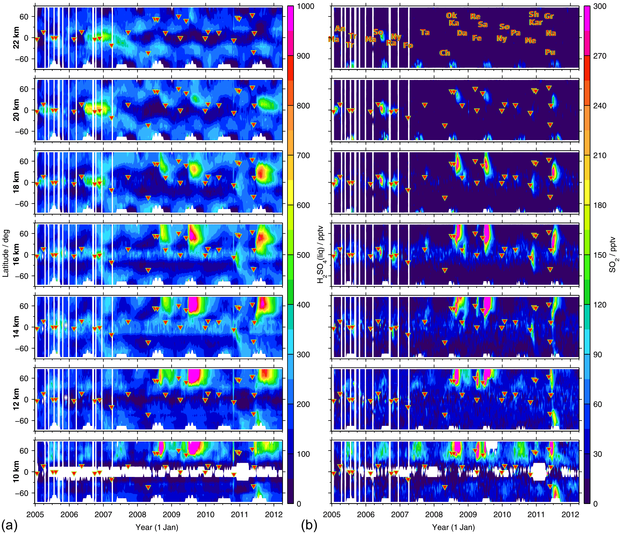
Figure 5Global time series of latitudinally resolved distributions of MIPAS liquid-phase H₂SO₄ (a) and SO₂ (b) volume mixing ratios. Shown are 8-day mean values for 10^∘ latitude bins at different altitudes (10 to 22 km). The colour code is restricted to 0–1000 pptv for H₂SO₄(liq) and 0–300 pptv for SO₂. Values exceeding these limits are assigned the limiting value. Volcanic eruptions are indicated by red triangles (together with their abbreviations in the uppermost image of panel (b); following Höpfner et al., 2015). Abbreviations: An – Anatahan; Ch – Chaitén; Da – Dalaffilla; Fe – Fernandina; Fo – Piton de la Fournaise; Gr – Grímsvötn; Ka – Kasatochi; Kar – Karymsky; Ma – Manam; Me – Merapi; Na – Nabro; Ny – Nyamuragira; Ok – Okmok; Pa – Pacaya; Pu – Puyehue–Cordón Caulle; Ra – Rabaul; Re – Redoubt; Sa – Sarychev; Sh – Shiveluch; So – Soufrière Hills; Ta – Jebel at Tair; Tr – unidentified tropical volcano.

Download

The latitudinally resolved time series of sulfate aerosol mole fractions further reveal different periodic structures, which are not connected to volcanic activities.

1. In polar regions at altitudes above ∼ 16 km, sulfate aerosol mole fractions decrease strongly in winter to spring. The pattern is more pronounced in the Southern Hemisphere. This decrease is connected to the polar vortex, where relatively sulfate-aerosol-free air is transported downwards. Thomason and Poole (1993) reported very low observed aerosol levels relative to non-vortex air.

2. In both hemispheres, but primarily in the Southern Hemisphere, mole fractions of liquid-phase H₂SO₄ are enhanced at around 20–22 km in the midlatitudes (and partly the tropics) during boreal/austral winter and spring. In the stratosphere sulfur is released from OCS mainly in the tropics at altitudes between about 25 and 35 km (Brühl et al., 2012), and the sulfate aerosol that is produced is transported towards midlatitudes and lower altitudes.

3. In the midlatitudes of the Northern Hemisphere, the sulfate aerosol is increased during boreal summer at around 10–12 km.

4. In the tropics at around 14–16 km aerosol values are elevated, while they are very low below and above these altitudes, unless influenced by volcanic eruptions.

As SO₂ is the main precursor for stratospheric sulfate aerosol during volcanically perturbed times, we analyse similarities and discrepancies between the distribution of latitudinally resolved time series of MIPAS SO₂ at various altitudes for 2005–2012 (Fig. 5b), and the new aerosol data (Fig. 5a). Prominent features seen in the distribution of SO₂ mole fractions from single limb scans are described by Höpfner et al. (2015). It should be noted that these data are useful mainly for the analysis of enhanced SO₂ rather than for background conditions, for which the monthly and zonal mean MIPAS SO₂ data set by Höpfner et al. (2013) is more suited. The distributions of SO₂ and sulfate aerosol show clear similarities, especially concerning volcanic plumes. Differences in the patterns result mostly from the longer residence time of sulfate aerosol in the stratosphere, compared to SO₂. Sulfate aerosol can reside in the stratosphere for several months up to several years if it is neither being transported back to the troposphere nor evaporated at higher altitudes. By contrast, SO₂ has a stratospheric lifetime of a few weeks. Different point sources, such as volcanic eruptions, can therefore be distinguished more easily in the SO₂ measurements than in the aerosol data. Further discrepancies arise from the fact that sulfur is released from SO₂ over weeks, during the exponential decay of the latter, and can then be converted into sulfate aerosol. Elevated SO₂ amounts therefore do not instantly lead to elevated sulfate aerosol amounts, and the curve of enhanced sulfate aerosol is broader and flatter than for SO₂.

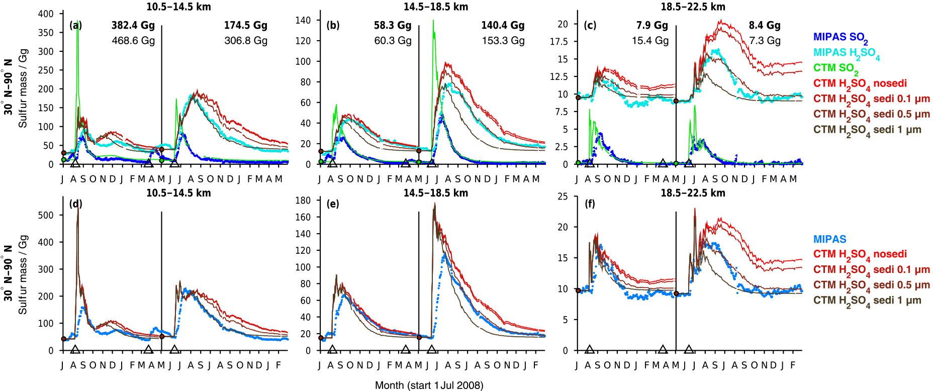
Figure 6Sulfur mass contained in SO₂ and sulfate aerosol after the eruptions of Kasatochi (7 August 2008) and Sarychev (12 June 2009) from MIPAS measurements and CTM simulations. Presented are 5-day running means for 30 to 90^∘ N, in three altitude regions (10.5–14.5, 14.5–18.5, 18.5–22.5 km). For the CTM four simulations for H₂SO₄(liq) are shown with different effective sedimentation radii (0.1, 0.5, and 1 µm) and without sedimentation. All simulations are carried out with the volcanic SO₂ masses from Table 1 (“present study”). A constant background SO₂ and aerosol loading is derived from the measured data and added to the simulated sulfur masses per altitude region (indicated by circles). Model simulations for Kasatochi and Sarychev are separated by a vertical black line in May 2009. (a–c) Sulfur mass per species. (d–f) Sum of sulfur mass in SO₂ and sulfate aerosol. The numbers in (a–c) show the peak values of sulfur mass contained in simulated SO₂ on locations covered by MIPAS (bold) and for all available model data. Indicated by black triangles are the eruption days of Kasatochi (7 August 2008; 52.2^∘ N, 175.5^∘ W), Redoubt (23 March 2009; 60.5^∘ N, 152.7^∘ W), and Sarychev (12 June 2009; 48.1^∘ N, 153.2^∘ E).

Download

In the Northern Hemisphere at low altitudes (< 12/13 km) during boreal summer, a similar feature of increased VMRs is present in the SO₂ as in the sulfate aerosol data (point 3). A closer look at the monthly distribution of SO₂ and sulfate aerosol reveals no distinct patterns (for SO₂, see Höpfner et al., 2015); enhancements are spread over the entire Northern Hemisphere. In Höpfner et al. (2015) this feature could not be confirmed due to a lack of SO₂ in situ data. The presence of similar enhancements in the aerosol data supports the hypothesis of the increased sulfur loading at low altitudes in the Northern Hemisphere not being a retrieval artefact. Further, elevated values in the tropics at around 14–16 km, as seen in the MIPAS aerosol (point 4) are also present in the SO₂ data. These are localised mostly in continental regions and the western Pacific, both for MIPAS sulfate aerosol and SO₂ (for SO₂, see Höpfner et al., 2015).

4.1 Sulfur mass in the Northern Hemisphere mid- and high latitudes

In this section we aim to test the agreement between measured SO₂ and liquid-phase H₂SO₄ masses, together with modelled data, in terms of the increase and decline in sulfur emitted by the volcanic eruptions of Kasatochi in August 2008 and Sarychev in June 2009, and the influence of the prescribed effective sedimentation radius on the residence time of sulfate aerosol. As we intend to test whether the measured aerosol is quantitatively and qualitatively consistent with its measured precursor by comparison with modelled sulfate aerosol, good agreement between the modelled and measured SO₂ masses is essential.

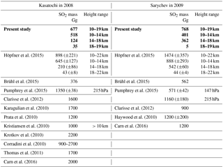
In Table 1 injected SO₂ amounts for three altitude regions are given (labelled “present study”), as used for the CTM simulations in the present study, together with comparisons to volcanic SO₂ masses from the literature. The upper injection limit for the volcanic emissions in the CTM is set to 19 km. Simulations have been made with varying injected SO₂ masses and upper injection altitude limits, intending to achieve good agreement between the modelled and measured SO₂ masses (comparisons as in Fig. 6). The data presented here resulted in the best agreement, with comparisons starting approximately 1 month after the respective eruption (explanation in the following). Due to the limited number of simulations no uncertainties are given for the presented SO₂ masses. The main part of SO₂ per eruption is emitted into the altitude region from 10 to 18 km, and only a few percent of the SO₂ masses are injected into altitudes above 18 km. Our best match for Kasatochi is consistent with the lower limit of Höpfner et al. (2015). Höpfner et al. (2015) derived volcanic SO₂ masses for three altitude regions from 10 to 14, 14 to 18, and 18 to 22 km by exponential extrapolation of the MIPAS SO₂ masses back to the eruption day. They applied this method as in the first month after the eruption MIPAS underestimates the SO₂ (Höpfner et al., 2015). Their method results in relatively large error bars that depend on the time period the fit is based on (Höpfner et al., 2015; presented also in Table 1). For Sarychev, however, our best estimate is smaller than the error limits of the SO₂ masses given by Höpfner et al. (2015).

When comparing the SO₂ masses from different studies, it has to be pointed out that the SO₂ masses are generally not derived for the same altitude regions. Höpfner et al. (2015), Brühl et al. (2015), and the present study are not totally independent of each other, as they are entirely or partly based on the same MIPAS SO₂ data by Höpfner et al. (2015). The SO₂ masses in our study lie below those of all studies except Brühl et al. (2015) for Kasatochi and in the range of the other publications for Sarychev. The wide range of SO₂ masses in Table 1 shows the difficulties and uncertainties related to the determination of volcanically emitted SO₂.

Table 1Volcanically emitted SO₂ masses from various publications for Kasatochi in 2008 and Sarychev in 2009. For Höpfner et al. (2015) the given total uncertainty is the sum of the uncertainties per altitude range (their Table 3). In the case of Pumphrey et al. (2015) pressure levels are given. These represent the highest pressure used for vertical integration. The SO₂ masses used in the present modelling study are indicated in bold.

Download Print Version | Download XLSX

Time series of sulfur mass contained in SO₂ and sulfate aerosol are shown in Fig. 6 for observations by MIPAS and simulations by the CTM. The sulfur loading is shown for three altitude regions, from 10.5 to 14.5, 14.5 to 18.5, and 18.5 to 22.5 km, for 30–90^∘ N, including the latitude of the eruptions (∼ 50^∘ N). For liquid-phase H₂SO₄ four model results are presented for each volcanic eruption. The simulations differ concerning the implemented sedimentation (no sedimentation and effective sedimentation radii of 0.1, 0.5, and 1 µm). In Fig. 6a–c, the sulfur mass is shown for SO₂ and sulfate aerosol separately, while Fig. 6d–f presents the total sulfur contained in SO₂ and sulfate aerosol. The total simulated sulfur mass is not influenced by chemical sulfur removal but only by removal due to transport by advection and sedimentation. In Fig. 6, the eruption times of Kasatochi (7 August 2008) and Sarychev (12 June 2009) are indicated. Additionally, the eruption time of Redoubt (23 March 2009) is marked, as this eruption produces a signal in the measurements. It is not included in the simulations, however.

To analyse the measured and simulated data, data sets of sulfur mass densities (SMD: mass per unit volume) are re-sampled on a common grid with 1 km vertical spacing and a horizontal resolution that equals the model grid. On this new grid, the same data basis is used for the measured and simulated data, neglecting all “grid cells” for which either only MIPAS or only CTM data are available. For MIPAS aerosols, SMDs are calculated from the primarily retrieved volume densities, using an assumed aerosol density of 1700 kg m⁻³ and a binary solution of 75 wt % H₂SO₄–H₂O, while for MIPAS SO₂ and the modelled values, SMDs are calculated from the mole fractions. Sulfur masses are then derived from 5-day running zonal means of SMDs, by multiplication with the corresponding air volume of the new grid.

Generally, when calculating an integrated mass, high data coverage is crucial to prevent underestimation; therefore, we use 5-day running zonal means. Zonal mean values, used to calculate sulfur masses, are derived using a method of increasing area averaging (see Appendix A) to reduce the bias of mean values due to a non-uniform data coverage. Even though high data coverage is very important, we omit available data and information, as the same basis of available values is used for MIPAS and the CTM. This is appropriate when analysing the agreement between the data. Data are omitted for the CTM in particular. Thus, we also provide some information on modelled sulfur masses derived from the non-co-located data (Fig. 6a–c). The impact of missing data is strongest in the lowermost altitude region presented here. For MIPAS this is mainly due to the presence of clouds and ash, which were filtered out using the cloud filter by Spang et al. (2004) in the case of SO₂ and partly filtered out in the case of aerosol; additionally, the ice and ash filters by Griessbach et al. (2016, 2014, respectively) were used for the aerosol retrieval. The CTM has low data coverage at lower altitudes due to its isentropic vertical grid. Interpolation to geometric heights starting at 10 km produces missing values at altitudes of up to 13 km.

To ease visual comparisons of measured and modelled sulfur mass in Fig. 6, a constant background is added to the model results, as only volcanic sulfur is considered in these simulations. The background mass is chosen considering the mass derived by MIPAS before the volcanic eruption in the region of interest per altitude and latitude bin. This does not necessarily represent normal background conditions but unmasks the anomalies caused by the volcanoes.

Concerning the measured and modelled SO₂ masses after the eruptions of Kasatochi and Sarychev (Fig. 6), comparisons show that until about 1 month after the eruptions, the SO₂ mass is by far underestimated by MIPAS. This underestimation of SO₂ was stressed by Höpfner et al. (2015) when comparing MIPAS SO₂ to measurements by the Microwave Limb Sounder (MLS) on board Aura (Pumphrey et al., 2015). It is mainly due to the presence of particles, which hinders MIPAS SO₂ measurements in largely eruption-affected air parcels and causes a sampling bias towards less volcano-affected air parcels. Through our model simulations we confirm this bias and the related timescale found by Höpfner et al. (2015). After this first month, the simulated SO₂ agrees well with the measurements by construction.

The measured decay of SO₂ is well reproduced by the CTM. Only oxidation by OH is considered in the model, and we see that the decay of SO₂ can adequately be described by this mechanism. Other processes, such as decay by photolysis or reaction with atomic oxygen (O), are not considered and, following the good agreement between measurements and model results, can be neglected on the temporal and spatial scale of interest. Inside volcanic plumes, chemistry interactions might lead to changes in SO₂ lifetimes (Bekki, 1995). When a high amount of SO₂ gets depleted by hydroxyl radicals, the concentration of the radicals might decrease, which could reduce the speed of further depletion. The good accordance between MIPAS measurements and CTM simulations, which do not account for any feedback on the OH concentrations, suggests that even if such interactions occurred, they did not produce a strong impact on the timescale of months and larger spatial scales.

To investigate the effect of particle sedimentation on the residence time of sulfur after the volcanic eruptions, model simulations with different effective sedimentation radii are performed, as well as one simulation without any sedimentation. The radii lie in the range of aerosol size distributions as observed by Deshler et al. (2003) and Deshler (2008) for volcanically perturbed periods, and one constant radius is applied for all H₂SO₄ droplets per simulation. Figure 6 shows the influence of varying the gravitational settling between no settling, and effective sedimentation radii of 0.1, 0.5, and 1 µm. The amount of sulfate aerosol removed by sedimentation increases with growing particle size, while the time needed for the removal increases for smaller effective sedimentation radii. The sulfur mass contained in liquid-phase H₂SO₄ from a simulation with an effective settling radius of 0.1 µm differs little from a simulation without sedimentation, while effective settling radii of 0.5 and 1 µm show an increasing impact. In the middle and uppermost altitude region, the best agreement between simulated and measured aerosols is found for an effective sedimentation radius of 0.5 µm for both eruptions. At 10.5–14.5 km, especially in the case of Sarychev, the simulations show temporal disagreement with the decrease in measured aerosol. In the lowermost altitude range, sparse data coverage has to be kept in mind, both for the measurements and model results. At these altitudes, sulfate aerosol simulated with a radius of 1 µm compares better. A larger effective sedimentation radius seems more appropriate at lower altitudes, as heavier particles can settle faster and can be removed more rapidly than smaller and lighter particles. These can float in the atmosphere or undergo ascent. The particle size distributions of aerosols can further show natural variation for different volcanic eruptions; therefore, some differences in the agreement between modelled and measured data when studying different volcanic eruptions can be expected. Model simulations show that compared to 10.5–18.5 km and compared to small particles, the bigger particles level out faster in the uppermost altitude range studied here. Reasons for this faster removal of the volcanic aerosol are that only little aerosol is injected in the altitude region of 18.5–22.5 km, that bigger particles settle faster, and that settling velocities rise with increasing altitude due to the corresponding decrease in air density. In general, we conclude that an effective settling radius of 0.5 µm gives a satisfactory fit between the measurements and simulations for the purpose of studying sulfur mass and sulfur transport in the Northern Hemisphere. Hence, we base all following model results on the CTM runs with an effective sedimentation radius of 0.5 µm.

We conclude from the comparisons between measured and simulated SO₂ and sulfate aerosol that the amplitude of the peak of liquid-phase H₂SO₄ and its removal from the studied altitude regions, as measured by MIPAS, is consistent with the measured SO₂, both qualitatively and quantitatively. In the model, sulfur is released from SO₂ due to its reaction with OH, and sulfate aerosol is consequently formed. Modelled SO₂ that fits MIPAS SO₂ measurements well in terms of amplitude and decay releases sulfur and builds H₂SO₄ that in turn matches MIPAS sulfate aerosol well in terms of amplitude and decrease.

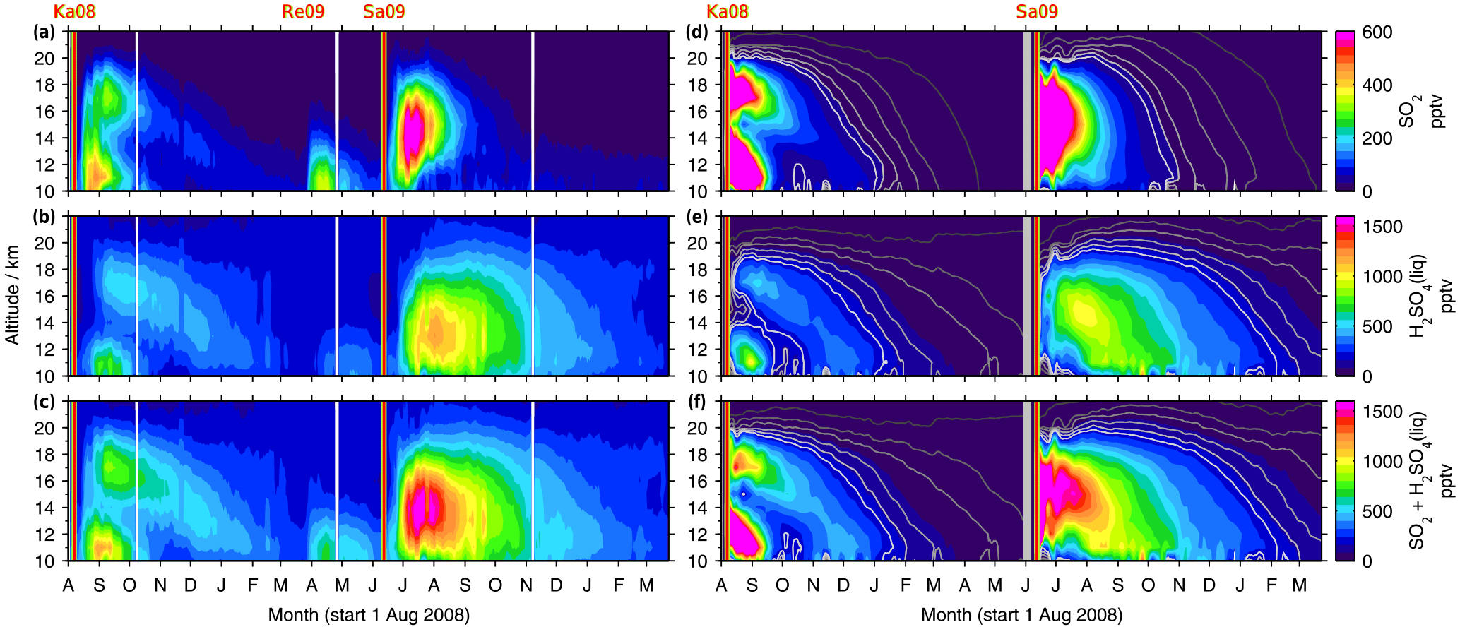
Figure 7SO₂, liquid-phase H₂SO₄, and total sulfur (SO₂ + H₂SO₄) volume mixing ratios by MIPAS (a–c) and the CTM (d–f). Vertically resolved time series of SO₂ and sulfate aerosol for 30–90^∘ N, starting on the 1 August 2008 (area weighted 5 d running means). Indicated are the days of the eruptions of the volcanoes Kasatochi in August 2008, Redoubt in March 2009, and Sarychev in June 2009, which were observed by MIPAS. Redoubt is not considered in the model. The colour scale is restricted to 0–800 pptv (SO₂) and 0–1600 pptv (sulfate aerosol and the sum of SO₂ and sulfate aerosol). Exceeding values are assigned the respective limiting value. The CTM contour lines in dark to light grey represent 1, 5, 10, 20, 30, and 40 pptv in the case of SO₂ and 5, 25, 50, 100, 150, and 200 pptv for sulfate aerosol and the sum of SO₂ and sulfate aerosol. For the CTM, two simulations are shown: from August 2008 to May 2009 and from June 2009 to May 2010, separated by a thick grey line.

Download

Further, we find that the dominating process on the evolution of volcanic sulfur is transport by the Brewer–Dobson circulation out of the region of interest. This becomes obvious when comparing the long-term removal of total modelled sulfur with and without sedimentation to the observed sulfur mass (Fig. 6d–f). In the case of the CTM, this excludes all influence by chemical reactions on the removal of volcanic sulfur. Even though a consideration of the sedimentation of sulfate aerosol with an effective sedimentation radius between about 0.5 and 1 µm further improves the agreement between model results and observations at 10–22 km altitude, the decay of modelled sulfur mass without sedimentation already compares rather well with the measured decay of sulfur mass. Hereby we see that the removal is dominated by advection rather than sedimentation.

A peak can be seen in the measured and modelled sulfur dioxide and sulfuric acid masses in November/December 2008 (Fig. 6) in the lowermost altitude region (10.5–14.5 km). This peak is caused by the downward transport of sulfur in the extratropics that has been emitted by the eruption of Kasatochi. In the following section (Sect. 4.2) more details are given on this transport pattern.

In the altitude region of interest, from around 10 to 22 km height, supplementary processes, such as the photolysis of gas-phase H₂SO₄, which is important at altitudes above 30 km (Vaida et al., 2003; Brühl et al., 2015), or a meteoritic dust sink (Brühl et al., 2015), are not considered. Other processes, such as the evolution of sulfate aerosol through microphysical processes (e.g. nucleation, coagulation, or condensation) and the sedimentation of particles with different sizes, can play a role in our region of interest. However, comparisons of simulations and measurements show that these processes are not essential for studying the development of sulfur emitted by Kasatochi in 2008 and Sarychev in 2009.

4.2 Sulfur transport

The Kasatochi eruption injected a large amount of SO₂ directly into the stratospheric altitude region especially between 10 and 14 km (Table 1). Figure 7 displays vertically resolved time series of SO₂ and liquid-phase H₂SO₄ mole fractions for 30^∘ N to 90^∘ N, as measured by MIPAS (7a–c) and modelled by the CTM (Fig. 7d–f), together with their sum (panels c and f). Both SO₂ and sulfate aerosol show a separation of the plume into a lower and upper part, in the measured and simulated data. While the lower part is removed relatively fast from the altitude range of observations, starting at 10 km, the upper part moves downward with time, following the Brewer–Dobson circulation. During the descent, the sulfur concentrations are reduced and some parts of the sulfur reach 10–12 km after several months. As the descent is seen in sulfate aerosol and SO₂, it is not primarily driven by sedimentation. A similar pattern of subsidence was found by Andersson et al. (2015, their Fig. 3) when studying aerosol scattering measured by CALIPSO (Cloud-Aerosol Lidar and Infrared Pathfinder Satellite Observations). The eruption of Sarychev in 2009 is also shown in Fig. 7. No separation of the plume is noticeable; vertically the sulfur is distributed rather homogeneously. In terms of downward transport from higher altitudes in the extratropics and the removal from the stratosphere, SO₂ and sulfate aerosol from the Sarychev eruption evolve in quite a similar way to the Kasatochi eruption.

Parts of the differences between the transport patterns after the eruptions arise from the injected SO₂ masses. In the case of Kasatochi, the main part of SO₂ was injected into altitudes below 14 km (518 Gg or 77 % of the injected SO₂). It is transported downwards and out of the region studied here relatively fast, and therefore only a minor part is reflected in the aerosol loading. In the case of the Sarychev eruption, almost half of the SO₂ (367 Gg or 48 % of the injected SO₂) is injected into the altitude region above 14 km. It is available for conversion into sulfate aerosol for a longer period of time, as can be seen in the higher H₂SO₄ volume mixing ratios after the eruption of Sarychev, compared to Kasatochi. Model simulations with “switched” SO₂ masses (mass of Kasatochi injected on the day and at the location of Sarychev, and vice versa) and a simulation with the SO₂ mass from the Kasatochi eruption injected at the location of Sarychev reveal that the “double plume” that was observed after the eruption of Kasatochi results from the combination of the vertical distribution of injected SO₂ masses and the prevailing transport after the 7 August 2008, the eruption date of Kasatochi, in the model driven by wind fields and heating rates. Neither of the simulations results in a comparable separation into an upper and lower part of the plume.

Figure 8As Fig. 7 but for 0–30^∘ N. The colour scales are restricted to 0–200 pptv (SO₂) and 0–800 pptv (sulfate aerosol and the sum of SO₂, and H₂SO₄(liq)). Additionally the volcano Dalaffilla is indicated in November 2008, as it was observed by MIPAS. It is not included in the model.

Download

Figure 8 shows vertically resolved measurements and simulations of SO₂ and liquid-phase H₂SO₄ for 0–30^∘ N. Some of the sulfur emitted at around 50^∘ N reaches low latitudes. While the SO₂ is removed rather fast, compared to sulfate aerosol, the sulfate aerosol resides in the tropics for many months and moves upwards with time. The modelled sulfate aerosol with an effective sedimentation radius of 0.5 µm behaves in a similar way as the measurements, moving slightly upwards with time. In comparison, a simulation with an effective sedimentation radius of 1 µm shows a rather horizontal transport and faster removal, while the simulated lifting is stronger than in the measurements when not considering sedimentation (not shown here). Due to uncertainties in modelled ascent speeds (e.g. Pommrich et al., 2010; Liu et al., 2013), the particle radius that is most suitable to reproduce MIPAS measurements by CTM simulations is not necessarily the best estimate when performing similar analyses with different models or meteorological driving data.

In the MIPAS data of the tropics, where the tropopause height is relatively constant at around 16–17 km, a clear transition from elevated sulfur mole fractions in the troposphere to lower sulfur loading in the stratosphere is observed during times of weak volcanic influence (May–June 2009; Fig. 8c). The relatively high values at around 13–16 km in the measurements have already been noted in Fig. 5 and are supposed to be only partly connected to volcanic eruptions. A certain influence of elevated retrieved aerosol values due to cirrus clouds that have not been captured by the ice filter (Sect. 3.1) is possible. It is not clear to what extent the observed enhancements in the measurements (Fig. 8a–c) are caused by the eruptions of Kasatochi and Sarychev. In the case of Kasatochi, model simulations suggest that enhancements are confined primarily to altitudes above approximately 16 km. Additionally to the tropical enhancements at 13–16 km, the eruption of Dalaffilla in November 2008 overlays the observed sulfur that has been emitted by Kasatochi. The CTM simulations of Sarychev indicate that sulfur observed at altitudes as low as 12 km can be attributed to the volcanic eruption.

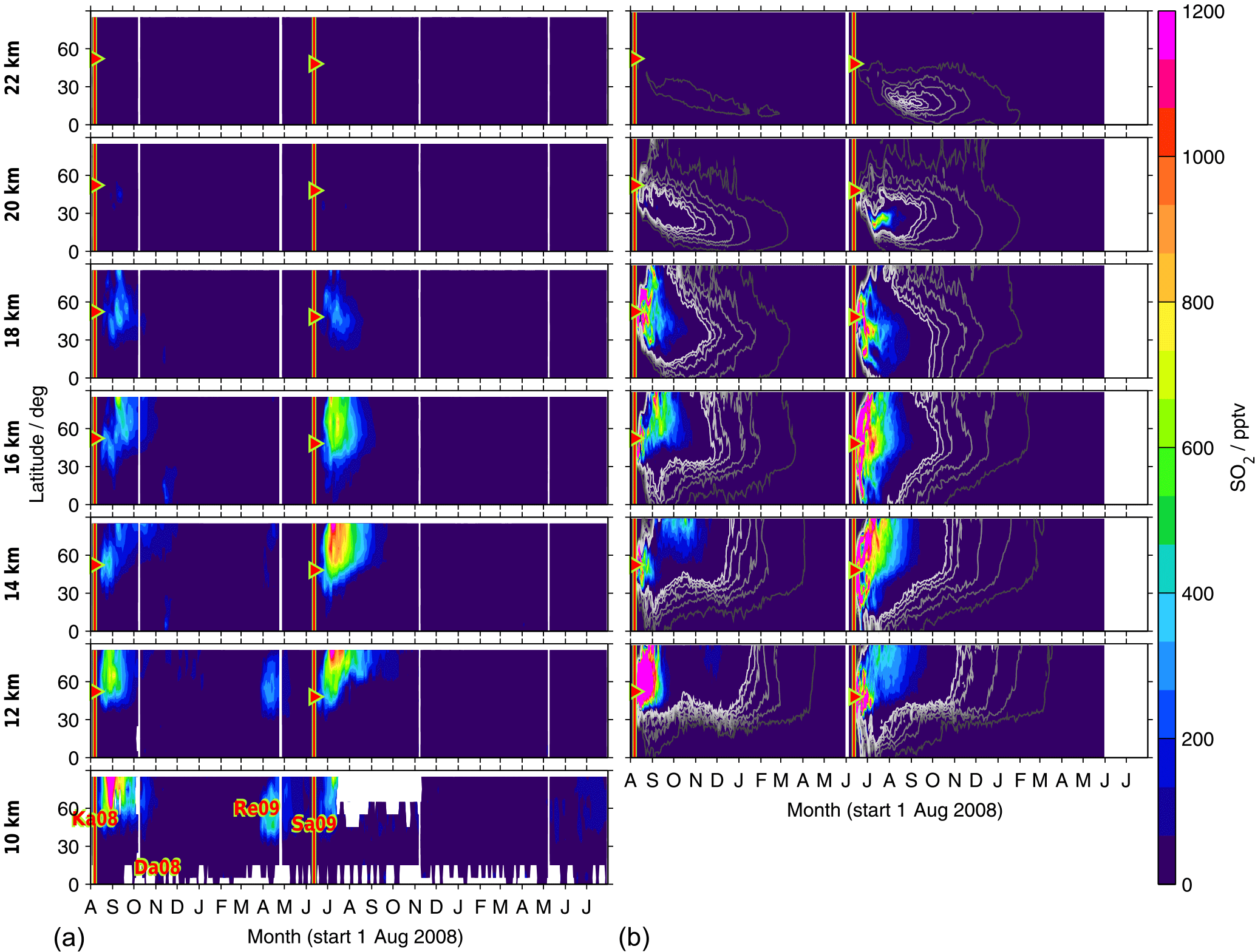
Figure 9Time series of SO₂ from MIPAS measurements (a) and CTM simulations (b). Shown are volume mixing ratios after the eruption of Kasatochi (7 August 2008) and Sarychev (12 June 2009), as zonal means for the Northern Hemisphere, at various altitudes (10 to 22 km). For MIPAS 5 d running means for 10^∘ latitude bins are calculated, while for the CTM daily values are shown for ∼ 2.5^∘ latitude bins. The colour code is restricted to 0–1200 pptv. Values exceeding these limits are assigned the limiting value. Time and location of the eruptions of Kasatochi and Sarychev are indicated by red triangles. (a) Indicated are the eruptions of Kasatochi and Dalaffilla in 2008 and Redoubt and Sarychev in 2009, which were observed by MIPAS. (b) The two simulations are separated by a vertical white line (1 June 2009). Black to white contour lines denote 1, 5, 10, 20, 30, and 40 pptv. Only Kasatochi and Sarychev are included in the model.

Download

Differences between the presented zonally averaged measurements and model results arise partly from the fact that MIPAS measurements are not uniformly distributed and data were filtered; they are also due to sparse data coverage in the case of the CTM up to an altitude of 12–13 km. Data are partly missing in relatively large areas, which may lead to biased zonal means. In the measurements, data for SO₂ are missing particularly in the tropics at altitudes below about 15/16 km and at higher altitudes (up to ∼ 17 km) in the region of the Asian summer monsoon. In the case of measured sulfate aerosol data are filtered especially in the tropics at altitudes of up to about 18/19 km and in the region of the Asian summer monsoon (up to ∼ 20 km), and in polar regions entire profiles were filtered out due to PSCs. After the eruption of Sarychev, in particular, a higher sulfur content is simulated in the tropics compared to the measurements (Fig. 8) and enhancements are seen few days after the eruption. This results from a strong modelled meridional transport of SO₂ after this eruption. At about 12–16 km altitude the injected SO₂ reaches 15^∘ N 7–8 d after the eruption. This strong southward transport early after the eruption is not reflected in the measurements, which are, however, partly missing in the tropics due to filtering.

In Figs. 9 and 10, time series of latitudinally resolved mole fractions show the transport of SO₂ and sulfate aerosol at different altitudes. We present time series of 5 d running zonal mean mole fractions for the Northern Hemisphere at altitudes from 10 to 22 km, both for MIPAS measurements and CTM simulations. As the model has low coverage at 10 km, results are not shown for the model at this altitude. For the eruption of Kasatochi, the separation of the plume and downward transport of the upper part is notable at mid- to high latitudes, most easily visible for sulfate aerosol (Fig. 10).

Figure 10As Fig. 9 but for sulfate aerosol. (b) Black to white contour lines denote 5, 25, 50, 100, 150, and 200 pptv.

Download

Both in the measurements and simulations, most of the sulfur contained in SO₂ and sulfate aerosol stays north of 30^∘ N at lower altitudes of up to around 16 km (Figs. 9 and 10). Especially at low altitudes we find a mixing barrier at ∼ 30^∘ N, with a strong gradient between low values in the tropics and high values in the extratropics, which weakens towards higher altitudes. This gradient is due to the subtropical jet stream and is most easily detectable in the contour lines shown for modelled liquid-phase H₂SO₄ (Fig. 10b), but similar patterns are observed by MIPAS. At around 16–18 km, especially in the longer-lived sulfate aerosol, this forms a “tongue” of relatively high mole fractions, which persists over a longer period than in the surrounding latitudes. At an altitude of about 18 km in the case of Kasatochi and ∼ 16 km in the case of Sarychev, and at altitudes above, a southward transport of sulfur is observed (Figs. 9 and 10). At these altitudes, both the MIPAS measurements and CTM simulations show that sulfur from midlatitude volcanic eruptions can reach the tropics, predominantly in the form of sulfate aerosol. In the tropics sulfur is then lifted in the “tropical pipe” (terminology following, e.g., Plumb, 1996) and can reach the stratospheric “overworld” (terminology following, e.g., Hoskins, 1991), also seen in Fig. 8. Measurements of the stratospheric optical depth by the Optical Spectrograph and InfraRed Imager System (OSIRIS) onboard Odin also show that in the months after the eruptions of Kasatochi in 2008 and Sarychev in 2009, their impact extended to lower latitudes (Bourassa et al., 2012). Wu et al. (2017) studied the equatorward dispersion of the Sarychev volcanic plume together with the influence of the Asian summer monsoon on the transport pattern. They find that at 360–400 K potential temperature, the southward transport was primarily caused by anticyclonic Rossby wave breaking, intensified by the Asian summer monsoon during Northern Hemisphere summer. Above 400 K less aerosol is transported into the tropics. They further show an “aerosol hole” in the anticyclone, surrounded by aerosol-rich air. Following Wu et al. (2017), a strong subtropical jet in combination with weak Rossby wave breaking events would hinder the southward transport of the volcanic plume during winter conditions. Compared to Sarychev, the southward transport of the Kasatochi eruption plume is weaker and initiates at higher altitudes. This might be explained by the eruption having been later during the monsoon season, leading to enhanced southward transport by the Asian summer monsoon for a shorter period of time. In model studies of the Sarychev eruption, Haywood et al. (2010) find that sulfate aerosol is transported around the entire globe in around 14 days. We see that the bulk of the aerosol that moves southwards reaches the Equator about 2 to 3 months after the volcanic eruption. To some small extent, this sulfur crosses the Equator and can thereby influence the sulfur loading of the Southern Hemisphere (see also Wu et al., 2017). Generally, similarities in the geographic pattern between Kasatochi in 2008 and Sarychev in 2009 have also been noticed by Haywood et al. (2010), caused by the agreement between the season, the injection altitude, and the latitude of the eruptions. The model results and MIPAS measurements of SO₂ and sulfate aerosol presented in our study confirm similarities in the transport patterns of sulfur after the volcanic eruptions of Kasatochi in August 2008 and Sarychev in June 2009 and a southward transport of the volcanic plumes, towards the Equator, where sulfur can then ascend in the Brewer–Dobson circulation.