the Creative Commons Attribution 4.0 License.
the Creative Commons Attribution 4.0 License.
 | 20 Aug 2018
Implementing microscopic charcoal particles into a global aerosol–climate model
Anina Gilgen
Carole Adolf
Sandra O. Brugger
Luisa Ickes
Margit Schwikowski
Jacqueline F. N. van Leeuwen
Willy Tinner
Ulrike Lohmann
Microscopic charcoal particles are fire-specific tracers, which are ubiquitous in natural archives such as lake sediments or ice cores. Thus, charcoal records from lake sediments have become the primary source for reconstructing past fire activity. Microscopic charcoal particles are generated during forest and grassland fires and can be transported over large distances before being deposited into natural archives. In this paper, we implement microscopic charcoal particles into a global aerosol–climate model to better understand the transport of charcoal on a large scale. Atmospheric transport and interactions with other aerosol particles, clouds, and radiation are explicitly simulated.
To estimate the emissions of the microscopic charcoal particles, we use recent European charcoal observations from lake sediments as a calibration data set. We found that scaling black carbon fire emissions from the Global Fire Assimilation System (a satellite-based emission inventory) by approximately 2 orders of magnitude matches the calibration data set best. The charcoal validation data set, for which we collected charcoal observations from all over the globe, generally supports this scaling factor. In the validation data set, we included charcoal particles from lake sediments, peats, and ice cores. While only the Spearman rank correlation coefficient is significant for the calibration data set (0.67), both the Pearson and the Spearman rank correlation coefficients are positive and significantly different from zero for the validation data set (0.59 and 0.48, respectively). Overall, the model captures a significant portion of the spatial variability, but it fails to reproduce the extreme spatial variability observed in the charcoal data. This can mainly be explained by the coarse spatial resolution of the model and uncertainties concerning fire emissions. Furthermore, charcoal fluxes derived from ice core sites are much lower than the simulated fluxes, which can be explained by the location properties (high altitude and steep topography, which are not well represented in the model) of most of the investigated ice cores.
Global modelling of charcoal can improve our understanding of the representativeness of this fire proxy. Furthermore, it might allow past fire emissions provided by fire models to be quantitatively validated. This might deepen our understanding of the processes driving global fire activity.
- Article
(3265 KB) -
Supplement
(610 KB) - BibTeX
- EndNote


Fires are an important component of the Earth system and are closely linked to vegetation. They reduce biomass, influence the distribution of biomes, and alter biodiversity (Bond and Keeley, 2005; Secretariat of the Convention on Biological Diversity, 2001). Furthermore, fires have a large impact on the atmosphere, mainly by emitting aerosol particles and greenhouse gases (Crutzen and Andreae, 1990) and to a smaller extent by altering the surface albedo (Gatebe et al., 2014). They threaten humans not only because of infrastructure and death risks but also because of carcinogenic smoke emissions (Stefanidou et al., 2008).
The biosphere, the atmosphere, and humans not only are impacted by fires but also influence them: the occurrence and size of fires strongly depend on the vegetation properties (e.g. vegetation structure and moisture), on some climate variables (e.g. lightning frequency, precipitation, temperature), and on human behaviour (e.g. land use changes, firefighting) (Hantson et al., 2016). In recent years, global fire models have become more advanced, but open questions still remain, e.g. regarding the complexity needed for global fire models (Hantson et al., 2016). Current fire models are generally tuned to match observations from recent decades, where satellite products give valuable information on the occurrence of fires. Thus, a major goal of current research is to test the fire models against palaeo-fire data (Rabin et al., 2017), which are independent of this tuning: only if the models are able to reproduce past conditions may they capture the key processes driving fires and provide trustworthy information about the future.
A number of natural archives provide information about palaeo-fires on different spatial and temporal scales. Sedimentary charcoal records from lakes and natural wetlands are unique because of the broad temporal and spatial coverage they provide, ranging from local to global and decadal to millennial scales (Whitlock and Larsen, 2001; Schüpbach et al., 2015). Recently, charcoal particles originating from ice cores have also been analysed (Isaksson et al., 2003). Beside charcoal particles, ice cores from glaciers and ice sheets also preserve other (potential) fire indicators such as black carbon (BC) or molecular fire tracers (Rubino et al., 2016). Due to their remote locations, ice cores can provide information on regional to subcontinental scale fire activity. Especially for the last ≈150 years, ice cores generally have a sound chronology and a high temporal resolution, which allows recent ice core data to be linked directly to coinciding satellite observations or fire simulations. This is an advantage of ice cores compared to other charcoal fire records, which are undated in some cases and often have multi-decadal resolutions only (with some exceptions such as sediment traps or varved sediments).
Charcoal particles differ from BC (as defined in the aerosol community; see e.g. Bond et al., 2013) in terms of formation mechanism, size, density, and H : C and O : C ratios (Preston and Schmidt, 2006; Conedera et al., 2009). BC condenses as a secondary product from hot gases present in flames, thereby forming aggregates of small carbon spherules. Characteristic for BC particles are their submicron sizes and their very high carbon content, the latter resulting in pronounced absorption of visible light. In contrast, charcoal particles retain recognisable anatomic structures of their biomass source, cover the range from submicron to millimetre scale, and have considerably higher H : C and O : C ratios than BC (i.e. containing less carbon and thus absorbing less radiation). Both particles have in common that they are formed during biomass burning and are considered to be rather inert, unreactive substances.
Charcoal particles can be divided into microscopic (DM>10 µm, where DM is the maximum dimension of the particle) and macroscopic (DM>100 µm) charcoal particles. In the most recent version of the Global Charcoal Database (GCDv3), more than a thousand sites with charcoal data are collected (Marlon et al., 2016). However, comparing data from the GCD with output from fire models is challenging: the collected charcoal data are only comparable to a certain degree due to differences in methods for extraction and counting, locations/environments, chronologies, particle sizes, values presented in percentages vs. concentrations or influx, etc. To circumvent the problem of inhomogeneous data, global synthesis studies such as Power et al. (2008) and Marlon et al. (2008) homogenised, rescaled, and standardised the data. The derived standardised scores (also called Z scores) enhance the comparability of the data but give only information about the relative changes of charcoal deposition. To estimate fire emissions from 1750 to 2015, van Marle et al. (2017) combined satellite retrievals, standardised scores from charcoal records, fire models, and visibility observations. The charcoal signal and the output from the fire models were scaled to match average regional GFED (Global Fire Emissions Database) carbon emissions from 1997 to 2003. However, to validate fire models and fire emission inventories, absolute values of charcoal fluxes (called influx or charcoal accumulation rate in the palaeo-science community) are still crucial.
To link the location of charcoal emissions (i.e. fires) with the fluxes derived at the observation sites (e.g. lake sediment), the transport of the particles must be taken into account. Previous studies have already investigated the transport of charcoal particles, which can take place in either air or water depending on site conditions and record type (e.g. Clark, 1988a; Peters and Higuera, 2007; Tinner et al., 2006; Lynch et al., 2004; Itter et al., 2017). Instead of explicitly modelling the transport, many of these studies chose a statistical approach.
In his pioneering study, Clark (1988a) focused on the transport of charcoal particles in air. He expected that the transport in fire plumes (which uplift particles to high altitudes) is responsible for nearly the whole long-range transport of microscopic charcoal particles. Clark (1988a) calculated that the transport of charcoal particles can be subcontinental to global: although charcoal particles are deposited relatively quickly due to their large sizes, their low density leads to considerably lower settling velocities compared to other supermicron particles (such as mineral dust).
More recently, Peters and Higuera (2007) and Higuera et al. (2007) used numerical models to simulate the major processes involved in macroscopic charcoal accumulation in lakes. Since they focused on charcoal particles from lake sediments, Higuera et al. (2007) considered not only fire conditions (size, location, and frequency) and transport but also sediment mixing and sediment sampling of macroscopic charcoal, while microscopic charcoal remained unexplored.
In the very recent study of Adolf et al. (2018), a uniform European data set of absolute charcoal fluxes is compared to satellite data of important fire regime parameters such as fire number, intensity, and burnt area at local and regional scales. Microscopic and macroscopic charcoal number fluxes are considered separately.
In this study, we explicitly simulate the aeolian transport and deposition of charcoal particles, which allows for quantitative comparison of simulated and observed charcoal fluxes. To model the transport of charcoal particles globally, we used the global aerosol–climate model ECHAM6.3-HAM2.3. We focus on microscopic charcoal particles, which primarily originate from fires in a radius of up to 100 km around the natural archive (Conedera et al., 2009) and are thus less influenced by specific site conditions (e.g. nearby burnable biomass). Part of microscopic charcoal particles can be transported over larger distances. For example, Hicks and Isaksson (2006) observed microscopic charcoal particles in Svalbard, which probably originated from the neighbouring continents and thus had been transported at least ≈1000 km.
Using a global aerosol–climate model allows the meteorological conditions for the transport to be calculated online. Furthermore, interactions of charcoal particles with other aerosol particles, with clouds, and with radiation can be considered. These factors might impact the removal processes of charcoal in the atmosphere and therefore where and when it is deposited.
Our main goals are to study the transport of microscopic charcoal particles on a global scale with a climate model and to test the model performance using charcoal data from different palaeo-fire records. The structure of this paper is the following: we first describe the charcoal data used for comparison with our simulations (Sect. 2). Subsequently, we describe the model, including the implementation of charcoal particles as a new aerosol species into our aerosol scheme (Sect. 3). In the “Results and discussion” section (Sect. 4), a comparison between model results and charcoal observations is shown as well as general atmospheric properties of the simulated charcoal particles such as mixing state. In the conclusions (Sect. 5), we summarise the key findings of this study.
In this study, aerosol fire emissions (including charcoal) were prescribed using a satellite-based emission inventory. Since the emissions of microscopic charcoal are unknown, we estimated them by scaling the fire emissions of BC and comparing the model result to European charcoal observations (calibration data set, Sect. 2.1). The derived scaling factor was then tested using different charcoal observations from various regions around the globe (validation data set, Sect. 2.2).
2.1 Data used for calibration
To calibrate our emissions, we used the data from Adolf et al. (2018). This data set comprises charcoal observations from 37 lake sediments all over Europe (see Table S1 in the Supplement). Compared to other parts of the world, biomass burning emissions from Europe are small. Nevertheless, we chose this data set because of its uniqueness: (i) annual fluxes are estimated very accurately owing to the use of sediment traps; (ii) due to the recent nature of the data (spring/summer 2012 to spring/summer 2015), it coincides with satellite-based fire emissions; (iii) it includes a sufficiently large number of observation sites; (iv) it covers a region sufficiently large to compare with a global model; and (v) all charcoal samples were prepared with the same technique, and all particles counted by the same person.
For nearly all sediments considered in this study, we can assume that the transport of charcoal takes place predominantly in air, not in water. However, for one lake in southern Spain (Laguna Zóñar) and one in Switzerland (Mont d'Orge), surface run-off is expected to be important because of the bare soil around the lakes. Surface run-off can transport deposited charcoal particles from the soil to the lake and thus enhance the number of charcoal particles in the sediment traps. Therefore, data from these two sites must be interpreted with caution.
Charcoal particles were counted in pollen slides with a magnification of 200–250×. Samples for microscopic charcoal analysis were treated following palynological standard procedures (Stockmarr, 1971; Moore et al., 1991). All black, completely opaque, and angular particles (Clark, 1988b) with a minimum DM of 10 µm and a maximum DM of 500 µm were counted following Tinner and Hu (2003) and Finsinger and Tinner (2005).
2.2 Data used for validation
To validate the model results, we used microscopic charcoal observations covering different parts of the world, which are independent of the calibration data set. Table S2 summarises the locations and the time (period) of the observations used for validation. Overall, data from 32 lake sediments and peats were compiled using the Alpine Pollen Database of the University of Bern (ALPADABA). While many charcoal observations from lake sediments and peats exist, charcoal particles have so far only been studied in a handful of ice cores (e.g. this study; Isaksson et al., 2003; Eichler et al., 2011; Reese et al., 2013). In our analysis, we include five ice core records. Three of them were obtained in the frame of the project “Paleo fires from high-alpine ice cores” (which also includes this study), in which charcoal data from the Eurocore 89, Greenland, were also analysed. One of them is from Belukha glacier, Siberian Altai (Eichler et al., 2011).
The selected data are as homogeneous as possible: to compare the data set with our simulated results, only number fluxes of charcoal particles with a lower threshold of DM=10 µm were considered. We excluded data using a different threshold or reporting no information from which we could calculate fluxes. Since the preparation technique also influences the estimated fluxes (Tinner and Hu, 2003), we furthermore ensured that the sample preparation and charcoal identification for the validation data set are identical to that of the calibration data set. The only exception is the data from Connor (2011). Instead of counting the number of charcoal particles above 10 µm, Connor (2011) measured the charcoal area following the method from Clark (1982). To compare it with the simulated number fluxes, the linear regression from Tinner and Hu (2003) for Lago di Origlio was applied to the observed data to convert charcoal area to number.
For the lake sediments and peats, we include additional information about the dating of the records in Table S2. The sediment age was used to calculate sediment accumulation rates. Based on the original chronologies, we assumed a linear sediment accumulation between the two youngest charcoal samples to calculate a sediment accumulation rate from which we then derived the charcoal flux for the uppermost sample of the record. By assuming a linear sediment accumulation, we may underestimate true values given that surface sediments are not compacted yet. The surface of the sediment core usually reflects the time of drilling. Therefore, the older the youngest dated point of the core, the larger the uncertainty of the most recent sediment accumulation rate and, consequently, the charcoal fluxes. Furthermore, the uncertainty of the fluxes depends on the dated material and the dating method (both listed in Table S2).
The ice cores considered for validation are derived from Colle Gnifetti (Switzerland), Tsambagarav (Mongolia), Belukha (Russia), Illimani (Bolivia), and Summit (Greenland), thus spanning a wide range of the globe. An exotic Lycopodium spore marker was added to the melted samples, which were then evaporated to reduce the volume and afterwards treated in the same manner as the standard sediment samples (Brugger et al., 2018).
We only take into account data that are more recent than 1980 in the validation data set as we had to find a compromise between including observations reflecting the fire conditions of the simulated period (2005–2014) and observations coming from many different locations but which are older than the simulation period.
3.1 Modelling charcoal particles in ECHAM6-HAM2
ECHAM6-HAM2 is a global climate model (ECHAM) coupled with an aerosol model (HAM) and a 2-moment cloud microphysical scheme. For more information about the model, we refer to Stier et al. (2005), Lohmann et al. (2007), Zhang et al. (2012), Stevens et al. (2013), and Neubauer et al. (2014). Since this is the first time that microscopic charcoal has been implemented into a global aerosol–climate model, in the following we will thoroughly describe which aspects need to be considered. First, we will describe general physical properties of microscopic charcoal and how these are represented by the model (Sect. 3.1.1). Second, we will describe how a life cycle of charcoal particles is simulated, i.e. from the emissions (Sect. 3.1.2) via atmospheric interactions (Sect. 3.1.3, 3.1.4) through to deposition (Sect. 3.1.5). In the end, some diagnostics complementary to the existing model output will be briefly mentioned (Sect. 3.1.6).
3.1.1 Size distribution, shape, and density
HAM uses the so-called M7 scheme (Vignati et al., 2004), which distinguishes seven aerosol modes classified by their size and solubility: soluble nucleation mode (number geometric mean radius rg<5 nm), soluble Aitken mode (), insoluble Aitken mode, soluble accumulation mode (), insoluble accumulation mode, soluble coarse mode (500 nm<rg), and insoluble coarse mode. Each of these modes is log-normally distributed, and the total aerosol particle size distribution is described by a superposition of the seven modes. To implement charcoal particles, we extended the scheme by two additional modes (M9 scheme), namely by a soluble giant and an insoluble giant mode. The giant mode has the same geometric standard deviation as the coarse mode (i.e. σg=2). We restricted neither the upper nor the lower bound of the giant mode, but the rg of the emitted (i.e. initial) size distributions was set between 0.5 and 5 µm (see Sect. 3.1.2). When a particle size distribution grows in M7, part of its mass and number is shifted to the next-larger mode, e.g. from the nucleation to the Aitken mode. To simplify diagnostics, we did not allow shifts from the coarse to the giant mode.
In HAM, all aerosol particles are assumed to be spherical. This condition is not fulfilled for charcoal particles, but at least microscopic charcoal particles seem to have a shape closer to a sphere than macroscopic charcoal particles (Crawford and Belcher, 2014). To compare our result with observations, we therefore use the volume-equivalent radius (req) of charcoal particles. To estimate req, the geometry of charcoal particles must be considered. Some studies analysed the shape of charcoal particles and reported their aspect ratios , where Dm is the minimum dimension of a particle. In the Supplement (Sect. S1.1), we summarise the findings concerning R in the literature. In our model simulations, we consider a range of R between 1.33 and 2.4 (corresponding to req of 4.9 and 3.5 µm); our initial estimate is R=2 (corresponding to req=3.9 µm).
A distinct characteristic of charcoal particles is their low density. Renfrew (1973) reports values of 0.3–0.6 g cm−3; Sander and Gee (1990) report similar values of 0.45–0.75 g cm−3. Hence, we chose a particle density of 0.5 g cm−3 as an initial guess, which lies in the middle of these ranges. For the test simulations, we considered values where both observations overlap, i.e. from 0.45 to 0.6 g cm−3.
3.1.2 Charcoal emissions
Thanks to fire emission inventories based on satellite data, we have a good knowledge about where and when fires of which sizes occurred in the last 1–2 decades. Nevertheless, aerosol emissions from fires are still uncertain. This is caused to a large degree by the pronounced variability of fires: emission factors (which relate the mass of the burnt vegetation to the mass of emitted aerosol particles) vary considerably depending for instance on vegetation type, fire temperature, or fire dynamics. To our knowledge, no study has estimated the emission factors of microscopic charcoal particles so far. Clark et al. (1998) and Lynch et al. (2004) focused on macroscopic charcoal when estimating mass emission fluxes; therefore these values are not comparable.
Airborne measurements of aerosol particles from fires usually have upper cutoff sizes of a few micrometres or less (e.g. Johnson et al., 2008; May et al., 2014). The aircraft measurements by Radke et al. (1990) are exceptional since they include particles with sizes up to 3 mm, therefore covering the whole size range of charcoal. In their study, they set three fires in North America. The measured particle size distribution showed similar shapes for all of these burns. Radke et al. (1990) report that a considerable fraction of the particles measured in the plumes were larger than 45 µm in diameter. From their data, we estimate that the mass emission fluxes of supermicron particles should be of the same order of magnitude as the mass emission fluxes of submicron particles, which is usually dominated by organic carbon (OC) in fire plumes (Desservettaz et al., 2017). Thus, we assume that all of these large particles are indeed charcoal and not ash or other large particles emitted from fires.
Since both BC and charcoal particles form under conditions when oxygen is limited in the burning process, we decided to scale BC mass emissions from fires to derive charcoal mass emissions. As a starting point for the scaling factor, we assume that the mass emission fluxes of microscopic charcoal are comparable to those of submicron particles. Since BC only contributes relatively little to the total submicron particle mass, we scale the BC mass by a factor ≈10 (based on the ratios of BC to total submicron particles and to OC; Desservettaz et al., 2017; Akagi et al., 2011; Sinha et al., 2003). Furthermore, scaling aerosol emissions from the Global Fire Assimilation System (GFAS) by a factor of 3.4 leads to a better agreement between simulated and observed aerosol optical depth for both the global Monitoring Atmospheric Composition and Change (MACC) aerosol system and ECHAM6-HAM2 (Kaiser et al., 2012; von Hardenberg et al., 2012). Therefore, we use a factor of as an initial estimate. Then we adjust this scaling factor until the simulated charcoal fluxes agree with the calibration data set (Sect. 2.1).
To describe the fire emissions, we use BC, OC, and SO2 mass emissions at a 3-hourly resolution by combining the daily emissions from GFAS (GFASv1.0 until September 2014, GFASv1.2 afterwards) with the daily cycle from GFED (year 2004; Kaiser et al., 2012; Mu et al., 2011). GFAS emissions are based on fire radiative power and make use of vegetation-specific aerosol emission factors following Andreae and Merlet (2001, with annual updates by Meinrat O. Andreae). The strongest spurious signals originating from industrial activity, gas flaring, and volcanoes should be masked. However, in our simulations we found unrealistically high charcoal emissions over Iceland. These “emissions” are most likely caused by lava, which emits a signal at the same wavelength at which fires are detected. As an example, the volcano Bardarbunga caused huge eruptions over Iceland in August/September 2014, coinciding with extremely high fire emissions in GFAS ( averaged between 62∘ N, 26∘ W and 67∘ N, 11∘ W for September compared to global mean emissions of for the same month). Therefore, we decided to mask all fire emissions over Iceland for our simulations. Furthermore, note that some fires are not detected by the satellite when clouds obscure the fire radiative power signal or when the signal is below the detection limit (which depends on the distance to sub-satellite track; Kaiser et al., 2012). Other uncertainties of biomass burning emissions include for example uncertainties in emission factors or land cover maps (Akagi et al., 2011; Fritz and See, 2008). More details about GFAS can be found in Kaiser et al. (2012).
Observations show that the larger the microscopic charcoal particles, the smaller their corresponding number concentration (e.g. Clark and Hussey, 1996). This implies that the number geometric mean radius rg of our emitted charcoal size distribution should be smaller than the lower threshold of microscopic charcoal detection (DM=10 µm); i.e. the observations rather lie on the descending branch of the emitted log-normal size distribution (see Fig. S2).
The airborne measurements by Radke et al. (1990) only show one clear maximum in the number size distribution at radius r=0.05 µm, which we attribute to aerosol particles other than charcoal (e.g. BC and OC). There is however a distinct flattening of the negative slope above r≈0.5 µm, which could well be caused by an increase in the charcoal particle number concentration. From the study by Clark and Patterson (1997), who analysed deposited charcoal distributions, we estimate that the number geometric mean radius is ≈5 µm (using R=2). Based on these two studies, we roughly estimate that the number geometric mean radius at emission lies in the range between 0.5 and 5 µm.
In contrast to the studies by Clark (1988a) and Higuera et al. (2007), our fire plume heights depend on the planetary boundary layer (PBL) height (Veira et al., 2015), which is illustrated in Fig. S1. If the PBL height is lower than 4 km, 75 % of the fire emissions are distributed between the surface and the model layer below the PBL height (at a constant mass mixing ratio), 17 % are injected in the first model layer above the PBL height, and 8 % are injected in the second layer above the PBL height. In the rare cases of the PBL height being larger than 4 km, the plume height is set to the PBL height and the emissions are equally distributed from the surface to the model layer below the PBL height.
We assume that all charcoal is emitted as insoluble, non-hygroscopic particles because of their rather high carbon content and inertness (Preston and Schmidt, 2006). Observations have shown that BC, which has an even higher carbon content than charcoal, can take up soluble material and then undergo further hygroscopic growth (Shiraiwa et al., 2007; Zhang et al., 2008). Hence, we assume that the same holds for charcoal particles, i.e. that charcoal particles can become internally mixed and thus be shifted to the soluble mode. This is explained in the following section.
3.1.3 Interactions with other aerosol particles
Charcoal particles can be shifted from the insoluble giant to the soluble giant mode by two processes: (i) Brownian coagulation with soluble particles from the nucleation or Aitken mode and (ii) condensation of sulfuric acid on the particle surface. Coagulation with larger modes is not considered because the Brownian motion of these particles is very low and coagulation is therefore not effective. Schutgens and Stier (2014) reported that even coagulation between the Aitken (BC, OC, sulfate) and the coarse mode (dust) is negligible, which suggests that the same might be the case for the Aitken and the giant mode (charcoal). Since charcoal particles – in contrast to dust – are co-emitted with BC, OC, and sulfate, we decided to nevertheless implement the coagulation between the giant and the Aitken mode. By coagulation, the aerosol species BC, OC, and sulfate can be transferred to the soluble giant mode. The soluble giant mode is therefore a mixture of different aerosol species, whereas the insoluble giant mode is exclusively comprised of charcoal.
In our model, the condensation of sulfate shifts the charcoal particle to the soluble mode when at least one mono-layer of sulfate covers the surface of the charcoal particle. Therefore, large charcoal particles are less likely to be transferred to the soluble mode by condensation of sulfate than small charcoal particles.
It is assumed that the soluble giant mode is internally mixed, i.e. that each individual aerosol particle consists of all components present in the mode. As soon as charcoal has been shifted to the soluble mode, the particles can grow further by water uptake when hygroscopic material like sulfate is present. In-cloud-produced sulfate mass can sometimes be added to the giant soluble mode when cloud droplets evaporate (see Sect. S2.1).
3.1.4 Interactions with microphysics and radiation
To our knowledge, the propensity of charcoal to act as a cloud condensation nucleus or ice-nucleating particle and the refractive index (RI) of microscopic charcoal have not been studied. In our model, mixed aerosol particles containing charcoal in the soluble giant mode can act as cloud condensation nuclei following the Abdul-Razzak and Ghan (2000) activation scheme. Charcoal itself does not dissociate. Further, we assume that charcoal particles cannot initiate freezing of cloud droplets. Concerning the interaction with radiation, we used the same RI as for dust; for explanation, see Sect. S1.2.
We do not expect these decisions to have a large impact on the atmospheric transport of charcoal particles since most charcoal particles do not reach levels where heterogeneous freezing becomes important, and the absorption of charcoal particles is likely too small to change the thermodynamic profile of the atmosphere.
3.1.5 Removal processes
Aerosol particles can be removed by three processes in HAM: wet deposition, gravitational settling, and dry deposition. Wet deposition in ECHAM6-HAM2 includes both in-cloud and below-cloud scavenging (Croft et al., 2009, 2010). Furthermore, the calculation distinguishes between liquid, mixed-phase, and ice clouds, as well as between stratiform and convective clouds. The wet-deposition calculation explicitly considers the sizes and the solubility of the aerosol particles. To prevent numerical instability, settling aerosol particles cannot fall through more than one model layer within one time step. However, this should not considerably change the spatial gravitational settling pattern (for details, see Sect. S2.2). In contrast to gravitational settling and wet deposition, dry deposition is only calculated near the surface. It accounts for the fact that a higher surface roughness leads to an increased aerosol flux to the surface because of turbulence. The surface roughness varies for different surface types, e.g. forest, water, or ice. Since gravitational settling is artificially slowed down near the surface on rare occasions (Sect. S2.2), dry deposition might take over and could therefore be somewhat overestimated.
3.1.6 Additional diagnostics
As mentioned in Sect. 3.1.2, we estimate the number geometric mean radius of the emitted charcoal size distribution to lie in the range 0.5–5 µm. This implies that a substantial portion of the simulated charcoal particles are smaller than Dm=10 µm and are therefore not included in the counts under the microscope. When comparing the simulated number fluxes to the surface with observations, we therefore want to exclude these small particles in our diagnostics. However, in the standard set-up of ECHAM6-HAM2, only the total surface fluxes for each giant mode are calculated. To circumvent this problem, we implemented additional diagnostics which calculate how many particles above a threshold radius are deposited. More information can be found in Sect. S2.3.
3.2 Model simulations
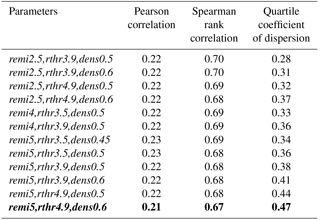
In this study, we used a model resolution of T63L31, which corresponds to a grid box size of ( at the Equator) with 31 vertical layers. For all simulations, we used a spin-up time of 3 months. We conducted test simulations to find suitable values for charcoal emission factors and three uncertain parameters described below. As mentioned previously, we increased the BC mass emissions by a scaling factor (SF) to estimate the charcoal emissions. These test simulations were nudged towards 6-hourly ERA-Interim data from April 2012 to May 2015 to cover the same time period as the calibration data set used to evaluate the model performance. First, three charcoal parameters were varied in the test simulations at a constant scaling factor (SF =34): the threshold radius (above which charcoal particles are counted), the emission number geometric mean radius, and the density. As an initial guess, we set the emission number geometric mean radius to req=2.5 µm, the threshold radius to req=3.9 µm (corresponding to R=2), and the density to 0.5 g cm−3. In Table 1, we refer to this simulation as remi2.5,rthr3.9,dens0.5. The values were varied in the ranges derived from the literature (see Sect. 3.1.2). Based on the comparison with the observations, we selected the best parameter set and then estimated which scaling factor is in best agreement with the observations.
Table 1Exemplary results of test simulations with different parameters (emission number geometric mean radius remi in µm, threshold radius rthr in µm, and density dens in g cm−3). The scaling factor is the same for all simulations (SF =34); the numbers hardly depend on the scaling factor. The parameters chosen for further simulations are marked in bold.
Finally, we conducted a nudged and a free simulation of 10 years each (January 2005 to December 2014) with the derived parameter set and scaling factor and compared our results with the observations described in Sect. 2.2.
For all simulations, we used 3-hourly fire emissions based on daily GFAS emissions (see Sect. 3.1.2). The other prescribed aerosol emissions are monthly means and do not show interannual variability. For most of these aerosol particles, we used present-day emissions (year 2000) from the Atmospheric Chemistry and Climate Model Intercomparison Project (ACCMIP; Lamarque et al., 2010). Dust, sea salt, and oceanic dimethyl sulfide emissions were calculated within the model at every time step.
To compare the simulations with the observations (e.g. calculating correlation coefficients), we used the SciPy package (Jones et al., 2001).
4.1 Calibration of emissions
We conducted test simulations and compared the result to the European observations from Adolf et al. (2018). Three measures were used for the comparison: (i) the Pearson correlation, which is a measure for linear correlation; (ii) the Spearman rank correlation, which assesses monotonic relationships; and (iii) the quartile coefficient of dispersion, which is a normalised and robust variability measure (, where Q1 and Q3 are the first and third quartiles, respectively). Table 1 shows some parameter combinations with positive correlation coefficients. In all test simulations, the correlation coefficients are very similar. While the Pearson correlation coefficients are low (0.21–0.23) and statistically insignificant, the Spearman rank correlation coefficients are much higher (0.67–0.69) and statistically significant. One reason for that is some observations with clearly larger charcoal fluxes than the simulated values (“outliers”) since the Pearson correlation coefficients are much more sensitive to outliers than the Spearman rank correlation coefficients. These outliers can nicely be seen in Fig. S4 for the example of remi2.5,rthr3.9,dens0.5. Two of them (black in Fig. S4) are sites expected to be influenced by surface run-off (Laguna Zóñar and Mont d'Orge), which explains the discrepancy between observations and model results. Removing these two points from the calculation causes the Pearson correlation to increase (e.g. from 0.22 to 0.26 for simulation remi2.5,rthr3.9,dens0.5). The other outliers (dots in Figs. S4 and S5 above 40000 on the y axis) are sites located in Sicily and southern France. A minor part of the deviation might be due to the proximity of these sites to the ocean. In this case, the grid boxes contain both land and ocean, which leads to an underestimation of charcoal emission fluxes over land in the model.
In all test simulations, we found that the variability of charcoal fluxes is clearly underestimated. We think that the two following reasons are mainly responsible for the larger variability in the observations compared to the model:
-
Model resolution. Sub-grid variability cannot be resolved by the model; i.e. the simulated emissions and depositions are an average over the whole grid box. In contrast, the observation sites can differ by a large amount, e.g. concerning the distance to burnable biomass, especially in the highly fragmented landscapes of Europe.
-
Uncertainties in fire emissions. Some fires might not be detected by the satellite (e.g. due to dense clouds) and therefore might not be accounted for in the simulated emissions. Furthermore, charcoal particle emissions could show a different variability concerning vegetation than BC does; i.e. the charcoal emissions per mass of burnt biomass might vary more between different vegetation types than we assumed.

Figure 1Simulated vs. observed number fluxes of charcoal particles above the threshold radius (in ) using the chosen estimate of parameters (an emission number geometric mean radius of req=5 µm, a threshold radius of req=4.9 µm, and a charcoal density of 0.6 g cm−3). The scaling factor increases from (a) to (d) (see legends). The two black dots show the sites likely influenced by surface run-off.
The quartile coefficients of dispersion (Table 1) show that the variability differs between the test simulations. The simulation with the highest variability (remi5,rthr4.9,dens0.6, albeit still having a lower variability than the observations) has only slightly lower correlation coefficients than the other simulations. Therefore, we choose this parameter set as the “best”. However, we are aware that choosing the parameter set with the highest variability might compensate for errors not related to the parameters (e.g. the model resolution) that are responsible for an underestimated variability. Furthermore, none of the parameter sets has a statistically significant Pearson correlation. Therefore, we cannot conclude from our simulations which parameter set is the most realistic one.
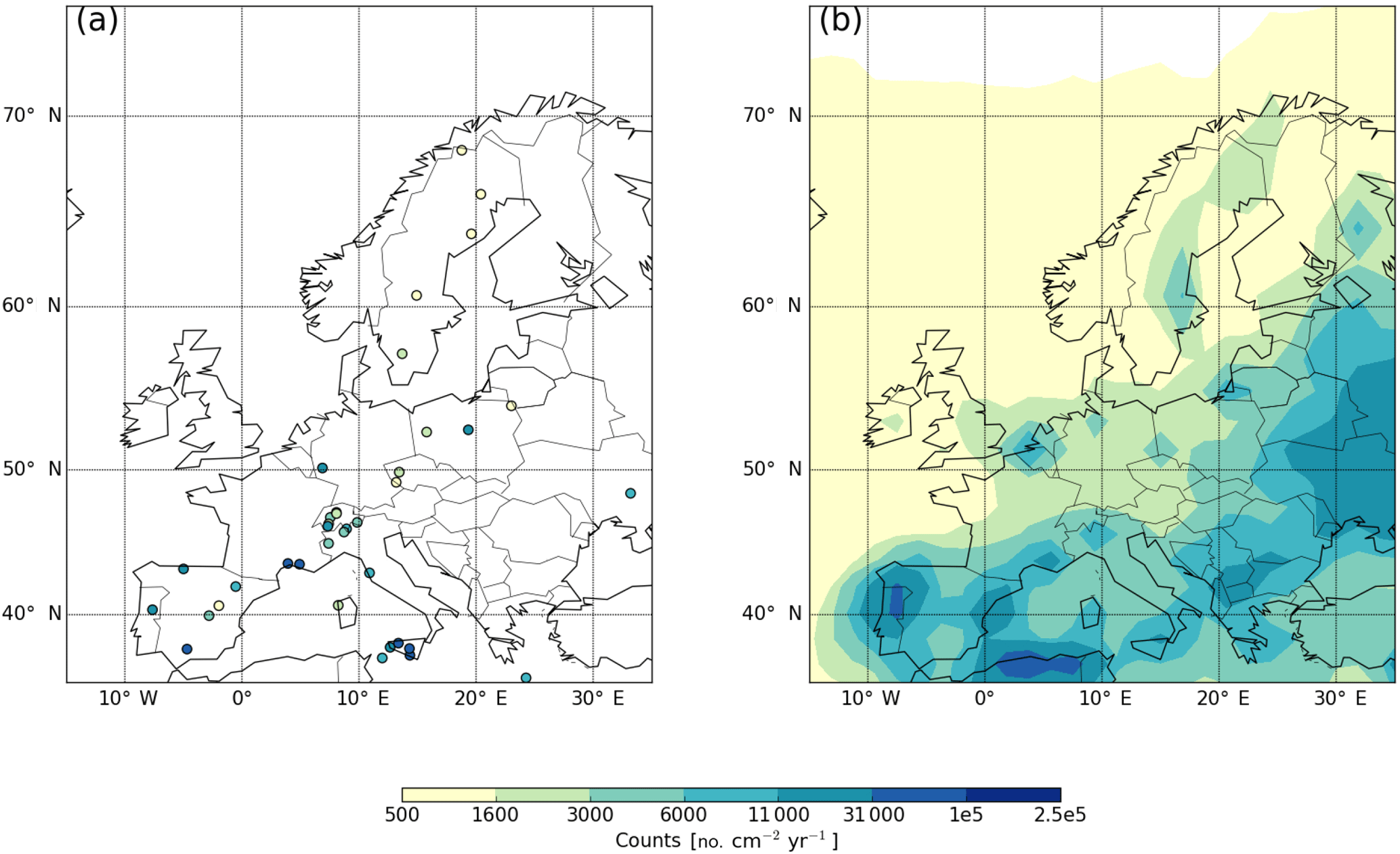
Figure 2(a) Observed vs. (b) simulated number fluxes of charcoal particles above the threshold radius (in ) using the chosen estimate of parameters (an emission number geometric mean radius of req=5 µm, a threshold radius of req=4.9 µm, and a charcoal density of 0.6 g cm−3).
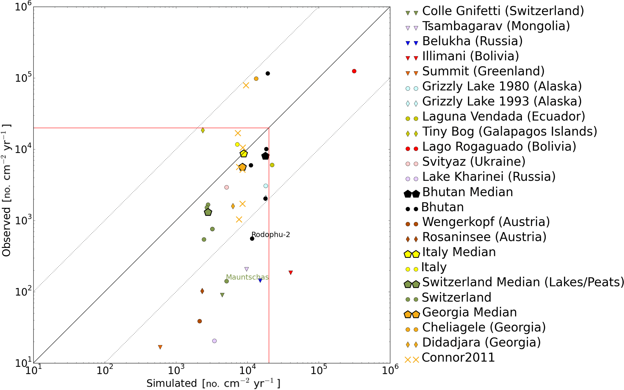
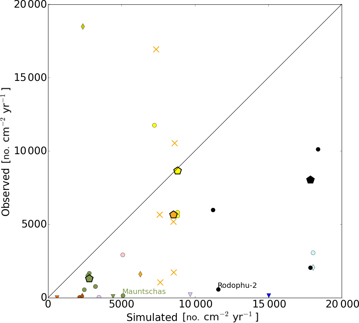
Figure 3Simulated vs. observed number fluxes of charcoal particles above a threshold radius of req=4.9 µm (in ) for the validation data set (with an emission number geometric mean radius of req=5 µm and a charcoal density of 0.6 g cm−3). The triangles refer to observations from ice cores; all other data are from sediments. The same colours are used for samples from the same countries. The data from Connor (2011) are distinguished by symbols (X's) because a different method was used. To improve readability, the different sediment observations from Bhutan, Italy, Switzerland, and Georgia are not further distinguished in the legend since the observation sites in these countries are close together. The median over them is illustrated by the large pentagrams. The red frame shows the axis limits of Fig. 4. The black solid line is the 1:1 line; the lines that are 1 order of magnitude away from the 1:1 line are dotted.
For the chosen parameter set (remi5,rthr4.9,dens0.6), we conducted simulations with different scaling factors (see Fig. 1). The correlation coefficients and the quartile coefficients of dispersion hardly depend on the scaling factor because charcoal particles do not coagulate with each other. We did not use the root mean squared error as a measure for the best scaling factor because the charcoal observations span several orders of magnitudes and the absolute deviations would be biased by the highest absolute charcoal fluxes (including the outliers). Instead, we consider the scaling factor for which approximately the same number of observations lies above and below the 1:1 line to be in best accordance with the observations. This is the case for a scaling factor of the order of SF =250 (see Fig. 1c), which furthermore has the smallest mean absolute error. However, note that the scaling factor depends on the chosen parameter set. Considering all parameter sets listed in Table 1, the best scaling factors range between SF ≈50 and ≈250.
Figure 2 shows the observed and the simulated charcoal fluxes over Europe. Overall, the model is able to capture the European north–south gradient in charcoal fluxes, with lower values in the north.
In the next section, we will validate the model with observations from different regions of the world.
4.2 Comparison with observations
In this section, we compare our simulated charcoal fluxes with independent observations. Here, we show results for the nudged 10-year model simulation; those of the free 10-year simulation are very similar (for comparison, Fig. S5 shows the same as Fig. 3 but for the free simulation). For the three ice cores spanning a recent multi-annual period, we average the model output over the same time periods (2005 to summer 2009 for Tsambagarav, 2005 to 2014 for Colle Gnifetti, and 2008 to 2014 for Illimani). For all other observations, we use the mean over the whole simulation for comparison.
As for the calibration simulations described in Sect. 4.1, the high variability in the observations is not reproduced by the model (see Fig. 3). For Bhutan, Italy, Switzerland, and Georgia, several lake sediment samples were collected in a small geographical region and are therefore not further distinguished in Fig. 3 (black, yellow, green, and orange symbols, respectively; medians over these samples shown as large pentagrams). The regional medians of the observations are rather close to the simulated median charcoal fluxes, indicating that the simulated fluxes are representative for a large scale. While the simulated median over Italy agrees very well with the observations, it is overestimated for Switzerland, Georgia, and Bhutan. Note that most of the data are also shown on a linear scale (Fig. 4), where we zoom in for better visibility (red frame in Fig. 3). The data from Connor (2011) (orange crosses) are the only ones originally measured in area fluxes and afterwards converted to number fluxes (see Sect. 2.2). The converted number fluxes compare well with the other observations and the model results, which indicates that the regression from Tinner and Hu (2003) can indeed be applied in this case.
Most simulated fluxes deviate by less than 1 order of magnitude from the observations, providing evidence that the simulated results are in good agreement with observed values at the sites. However, the charcoal flux values are highly overestimated for all ice cores (triangles), for three peats in the Alpine region (Mauntschas, Rosaninsee, and Wengerkopf), and for the sediment from Lake Kharinei (northern Russia). The model probably overestimates the fluxes at the ice core sites because of their high location within complex topography. The model is not able to simulate these high locations correctly since the surface altitude is constant over the whole grid box; i.e. the topography is smoothed. The simulated grid box averages are therefore not comparable to the ice core measurements. In reality, ice cores are located above the top plume height of most fires (Rémy et al., 2017), which may prevent transport of charcoal particles to them. Furthermore, the simulated fire emission height has a bias towards higher plume heights (Veira et al., 2015), which likely also contributes to the overestimation of simulated charcoal fluxes for sites above 4000 m (Rodophu-2 and all ice cores except Greenland). In addition, we expect that this bias leads to an overestimation of the simulated transport of charcoal to remote locations, which could explain the high simulated fluxes at Lake Kharinei and in Greenland. Another explanation for the overestimated simulated fluxes in Greenland is an increase in fire activity: GFAS data between 2003 and 2015 suggest that the fire emissions in Greenland might have increased in recent years. Fire activity was recorded in the years 2003, 2007, and all years from 2011 onwards, with highest aerosol emissions occurring in 2015. Therefore, it is possible that the fire activity was lower in 1989 (when the ice core was drilled) than in the simulated period (2005–2014). For the alpine sites, the observed fluxes might again not be representative for the whole grid box due to the small-scale, heterogeneous landscape around these observation sites (fire emissions and vegetation cover are constant in one model grid box).
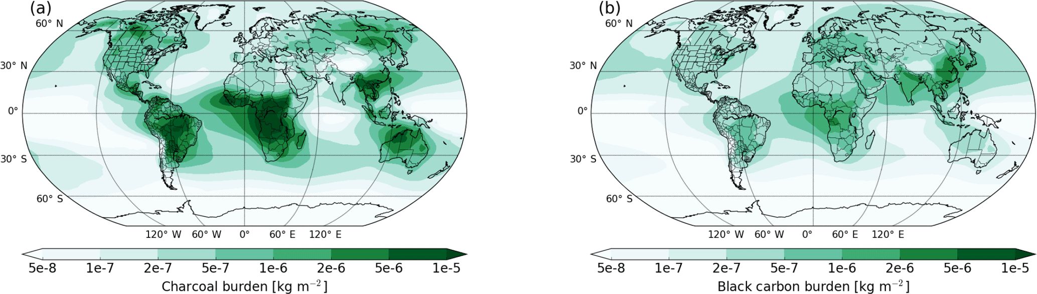
Figure 5Simulated aerosol burden averaged over 10 years for (a) charcoal and (b) black carbon. For the charcoal burden, only particles above the threshold radius of req=4.9 µm are considered. A charcoal emission number geometric mean radius of req=5 µm and a charcoal density of 0.6 g cm−3 were used.
Overall the chosen scaling factor (SF =250) describes the data well; i.e. a global charcoal scaling factor seems to be justified. However, the validation data set does not cover certain regions (e.g. Africa or Australia) and is biased towards northern mid-latitudes. The correlation between observed and simulated fluxes is 0.59 and 0.48 for the Pearson and the Spearman rank correlation, respectively, and in both cases statistically significant.
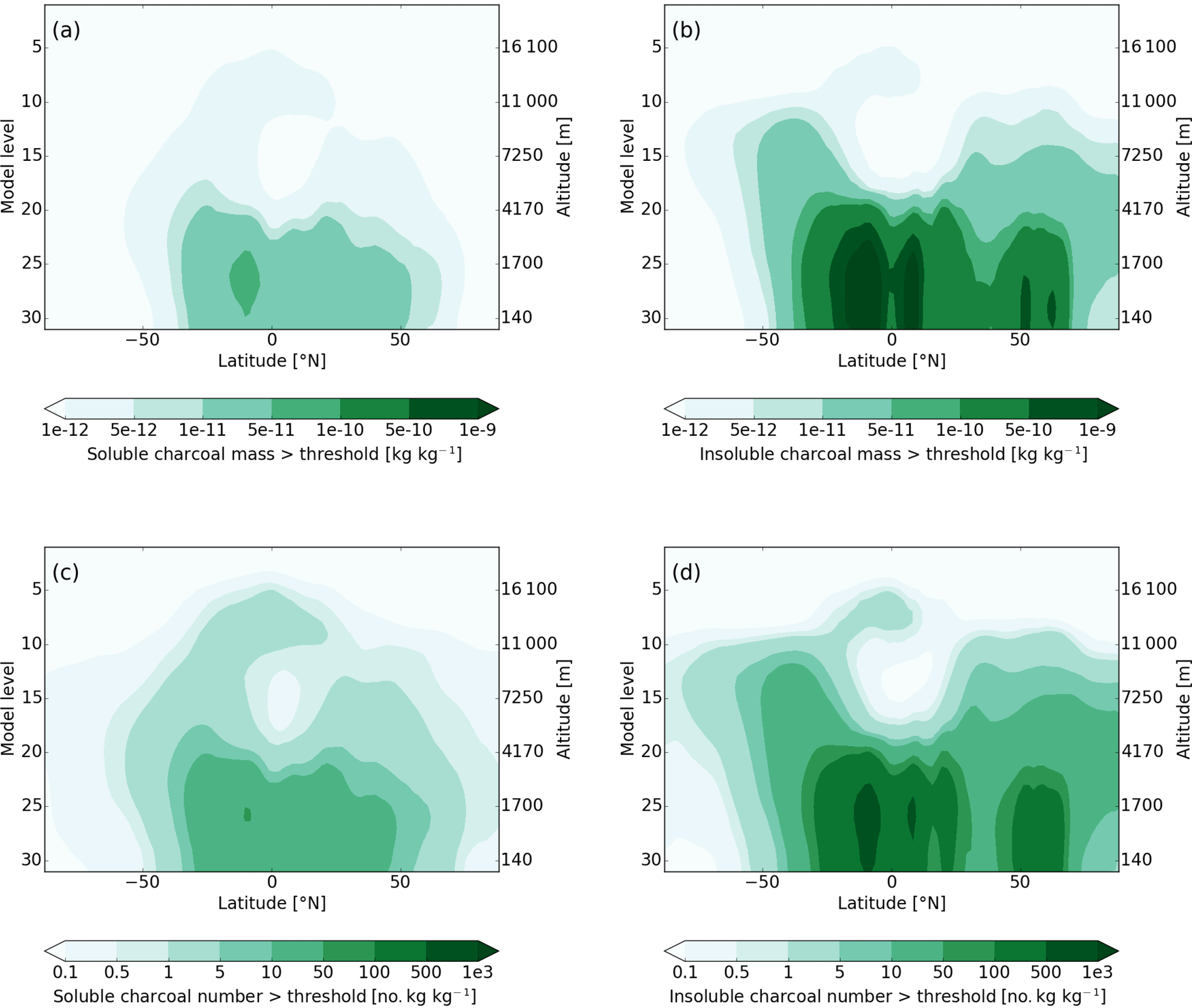
Figure 6Ten-year zonal average of the charcoal mass concentration above the threshold radius (req=4.9 µm) in (a) the soluble and (b) the insoluble giant mode and of the number concentration of (charcoal) particles above the threshold radius in (c) the soluble mode and (d) the insoluble giant mode (using an emission number geometric mean radius of req=5 µm and a charcoal density of 0.6 g cm−3). The right y axis shows to which altitude the model layers approximately correspond.
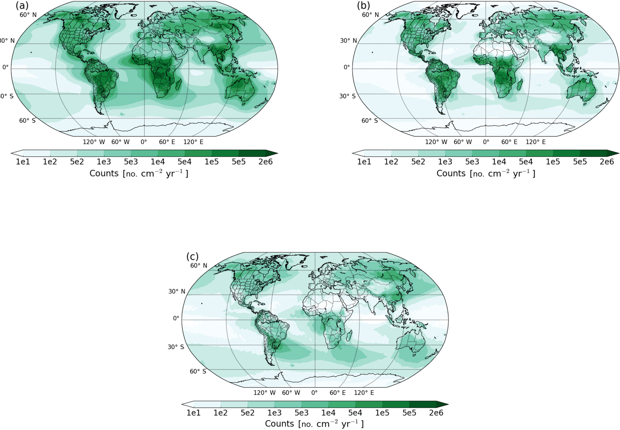
Figure 7The number fluxes (number of particles above a threshold radius of req=4.9 µm in ) of the three different charcoal removal processes in the model (with an emission number geometric mean radius of req=5 µm and a charcoal density of 0.6 g cm−3): (a) gravitational settling, (b) dry deposition, and (c) wet deposition.
4.3 Global distribution considering all microscopic charcoal particles
The global microscopic charcoal burden, i.e. the vertically integrated mass of microscopic charcoal particles in the atmosphere (above the threshold radius), is shown in Fig. 5a averaged over the 10-year nudged simulation. As expected, the burden is highest where most biomass burning emissions occur, namely in the tropics followed by the northern high latitudes (mainly Siberia and North America; Kaiser et al., 2012). The simulated global mean burden above the threshold radius is kg m−2, i.e. approximately 6 times larger than the burden of BC, which is kg m−2 including all BC sources and sizes (shown in Fig. 5b). Although the largest charcoal burdens occur near the emission sources, significant fractions of charcoal mass are transported hundreds of kilometres in the model, which is for example the case near the east coast of North America or the west coast of central Africa.
Most of the charcoal above the threshold radius resides in the insoluble mode in terms of number and mass, and only a few percent is shifted to the soluble mode (see Fig. 6). The small contribution of the soluble mode can be explained by the large size of the charcoal particles (limiting amount of coating material) and the related short atmospheric lifetime. Beside charcoal, the soluble mode is predominantly comprised of sulfate (and water), while the mass contributions of BC and OC are small (not shown).
4.4 Deposition of microscopic charcoal particles
As expected, the different atmospheric removal processes for charcoal particles above the threshold radius differ in geographic distribution (see Fig. 7). While gravitational settling and dry deposition become less important the larger the distance to the emission source, this is not generally the case for wet deposition. Large wet-deposition fluxes are observed where (simulated) precipitation is high, e.g. along the Atlantic storm track. Contrary to gravitational settling, dry deposition depends on the surface properties (Stier et al., 2005). Therefore, dry-deposition fluxes are small over the ocean compared to over land.
Overall, gravitational settling is the most important removal process, followed by dry deposition and then wet deposition. Although gravitational settling and dry deposition dominate the global charcoal deposition, wet deposition is the dominant removal process in some remote regions like part of Greenland.
Charcoal records from lake sediments are widely used to reconstruct past fire activity. More recently, charcoal particles have also been studied in ice cores. In this paper, we implemented microscopic charcoal particles into a global aerosol–climate model. Comparing simulated with observed charcoal fluxes might help to quantitatively reconstruct past fire activity. A recent and comprehensive charcoal data set from Europe was used for calibration of model emissions. Increasing BC fire emissions by a factor of 250 resulted in the best match between the model and observations, but this scaling factor depends on the chosen parameter set (ranging from ≈50 to ≈250 for the parameter sets that we tested). Although the model is not able to reproduce the high local variability of the observations, it captures the large-scale pattern of charcoal deposition (e.g. the north–south gradient in Europe) reasonably well. The charcoal fluxes for the validation data set, which covers different locations across the globe, are well captured with the constant charcoal scaling factor derived from the European calibration data set. However, our validation data set consists mostly of samples from northern mid-latitudes. We also found an underestimation in variability for the validation data set but a positive, statistically significant correlation between modelled and observed fluxes. The model shows a systematic positive bias for the ice core observations, which is likely due to the high altitude of the ice core sites as well as the complex topography around them.
As expected, the largest simulated charcoal deposition fluxes occur near fires. However, the model suggests that a non-negligible amount of microscopic charcoal particles is transported over large distances and therefore reaches remote locations (although comparisons with observations indicate that the model might overestimate long-range transport). In the model, only a few percent of charcoal particles is mixed with soluble material in the atmosphere.
The Global Paleofire Working Group (Hawthorne et al., 2017) aims for more standardised charcoal observations that cover all relevant fire regions. Here we suggest that more systematic and standardised observations of microscopic charcoal as number fluxes (with e.g. maximum particle dimension >10 µm, as in Adolf et al., 2018) could help to improve data–model comparisons and to verify whether a constant scaling factor indeed describes the data well on a global scale. In future studies, our new framework allows global modelling of charcoal and other biomass-burning-relevant tracers such as black carbon, which may improve the understanding of the representativeness of individual fire proxies. In addition, simulating microscopic charcoal particles using the scaling factor found might allow us to quantitatively validate past fire emissions provided by fire models. The validation of fire models is essential to improve the understanding of the key drivers of fires and to gain confidence in projections of future fire activity.
The ECHAM-HAMMOZ model is made freely available to the scientific community under the HAMMOZ Software Licence Agreement, which defines the conditions under which the model can be used. More information can be found at the HAMMOZ website (https://redmine.hammoz.ethz.ch/projects/hammoz, ECHAM-HAM(MOZ) developers, 2018).
You can find the data at https://data.iac.ethz.ch/Gilgen_et_al_2018_Charcoal (Gilgen, 2018).
The supplement related to this article is available online at: https://doi.org/10.5194/acp-18-11813-2018-supplement.
AG did most of the programming, conducted the simulations, and wrote the main part of the manuscript, with major contributions from SOB and CA to Sect. 2 and contributions from all authors to the text. MS, WT, and UL designed the overall project, while AG, LI, and UL were responsible for the details about the charcoal implementation in the model. CA collected the data from Laguna Vendada and provided the data set used for calibration. SOB compiled and processed most of the data used for validation, contributed a great deal to the discussions about the comparison between the model and the observations, and provided unpublished ice core data. JFNvL provided unpublished data from Cheliagele, Svityaz, Tergang, Shamling, Rodophu-2, Laya, Tiny Bog, and Lake Hallwil. All authors provided valuable comments to the manuscript.
The authors declare that they have no conflict of interest.
We thank the Swiss National Science Foundation (SNF) for granting the
Sinergia project “Paleo fires from high-alpine ice cores”, which funded
this research and enabled the collaboration between different research
disciplines (CRSII2_154450). This work was also supported by a grant from
the Swiss National Supercomputing Centre (CSCS) under project ID s652. In
addition, we are grateful to Michael Sigl and Dimitri Osmont from the Paul
Scherrer Institute for helping with the ice core preparation. Furthermore, we
acknowledge the help of W. O. van der Knaap from the University of Bern,
who extracted the raw data from ALPADAPA, and Peter Kunes, who counted the
charcoal particles from Singhe Dzong. We are also thankful to Thomas Blunier
from the Centre for Ice and Climate in Copenhagen; he kindly provided us
ice from the Summit ice core. We generally thank the developers of
ECHAM-HAM(MOZ), who continuously improve the model. The ECHAM-HAMMOZ model is
developed by a consortium composed of ETH Zürich, Max Planck Institut für
Meteorologie, Forschungszentrum Jülich, the University of Oxford, the Finnish
Meteorological Institute, and the Leibniz Institute for Tropospheric
Research, and managed by the Center for Climate Systems Modeling (C2SM) at
ETH Zürich. Last but not least, we acknowledge the critical and essential
comments from Brian Magi and an anonymous reviewer.
Edited by: Frank Dentener
Reviewed by: Brian
Magi and one anonymous referee
Abdul-Razzak, H. and Ghan, S. J.: A parameterization of aerosol activation: 2. Multiple aerosol types, J. Geophys. Res.-Atmos., 105, 6837–6844, https://doi.org/10.1029/1999JD901161, 2000. a
Adolf, C., Wunderle, S., Colombaroli, D., Weber, H., Gobet, E., Heiri, O., van Leeuwen, J. F. N., Bigler, C., Connor, S. E., Gałka, M., La Mantia, T., Makhortykh, S., Svitavská-Svobodová, H., Vannière, B., and Tinner, W.: The sedimentary and remote-sensing reflection of biomass burning in Europe, Global Ecol. Biogeogr., 27, 199–212, https://doi.org/10.1111/geb.12682, 2018. a, b, c, d
Akagi, S. K., Yokelson, R. J., Wiedinmyer, C., Alvarado, M. J., Reid, J. S., Karl, T., Crounse, J. D., and Wennberg, P. O.: Emission factors for open and domestic biomass burning for use in atmospheric models, Atmos. Chem. Phys., 11, 4039–4072, https://doi.org/10.5194/acp-11-4039-2011, 2011. a, b
Andreae, M. O. and Merlet, P.: Emission of trace gases and aerosols from biomass burning, Global Biogeochem. Cy., 15, 955–966, https://doi.org/10.1029/2000GB001382, 2001. a
Bond, T. C., Doherty, S. J., Fahey, D. W., Forster, P. M., Berntsen, T., DeAngelo, B. J., Flanner, M. G., Ghan, S., Kärcher, B., Koch, D., Kinne, S., Kondo, Y., Quinn, P. K., Sarofim, M. C., Schultz, M. G., Schulz, M., Venkataraman, C., Zhang, H., Zhang, S., Bellouin, N., Guttikunda, S. K., Hopke, P. K., Jacobson, M. Z., Kaiser, J. W., Klimont, Z., Lohmann, U., Schwarz, J. P., Shindell, D., Storelvmo, T., Warren, S. G., and Zender, C. S.: Bounding the role of black carbon in the climate system: A scientific assessment, J. Geophys. Res.-Atmos., 118, 5380–5552, https://doi.org/10.1002/jgrd.50171, 2013. a
Bond, W. and Keeley, J.: Fire as global “herbivore”: The ecology and evolution of flammable ecosystems, Trends Ecol. Evol., 20, 387–394, 2005. a
Brugger, S. O., Gobet, E., Schanz, F. R., Heiri, O., Schwörer, C., Sigl, M., Schwikowski, M., and Tinner, W.: A quantitative comparison of microfossil extraction methods from ice cores, J. Glaciol., 64, 432–442, https://doi.org/10.1017/jog.2018.31, 2018. a
Clark, J. S.: Particle motion and the theory of charcoal analysis: Source area, transport, deposition, and sampling, Quaternary Res., 30, 67–80, https://doi.org/10.1016/0033-5894(88)90088-9, 1988a. a, b, c, d
Clark, J. S.: Stratigraphic charcoal analysis on petrographic thin sections: Application to fire history in northwestern Minnesota, Quaternary Res., 30, 81–91, https://doi.org/10.1016/0033-5894(88)90089-0, 1988b. a
Clark, J. S. and Hussey, T. C.: Estimating the mass flux of charcoal from sedimentary records, The Holocene, 6, 129–144, 1996. a
Clark, J. S. and Patterson, W. A.: Background and Local Charcoal in Sediments: Scales of Fire Evidence in the Paleorecord, Springer Berlin Heidelberg, Berlin, Heidelberg, 23–48, https://doi.org/10.1007/978-3-642-59171-6_3, 1997. a
Clark, J. S., Lynch, J., Stocks, B. J., and Goldammer, J. G.: Relationships between charcoal particles in air and sediments in west-central Siberia, The Holocene, 8, 19–29, https://doi.org/10.1191/095968398672501165, 1998. a
Clark, R.: Point count estimation of charcoal in pollen preparations and thin sections of sediments, Pollen et Spores, 24, 523–535, 1982. a
Conedera, M., Tinner, W., Neff, C., Meurer, M., Dickens, A. F., and Krebs, P.: Reconstructing past fire regimes: methods, applications, and relevance to fire management and conservation, Quaternary Sci. Rev., 28, 555–576, https://doi.org/10.1016/j.quascirev.2008.11.005, 2009. a, b
Connor, S. E.: A Promethean Legacy: Late Quaternary Vegetation History of Southern Georgia, the Caucasus, Peeters, Louvain, 2011. a, b, c, d
Crawford, A. and Belcher, C.: Charcoal Morphometry for Paleoecological Analysis: The Effects of Fuel Type and Transportation on Morphological Parameters, Appl. Plant. Sci., 2, 1–10, https://doi.org/10.3732/apps.1400004, 2014. a
Croft, B., Lohmann, U., Martin, R. V., Stier, P., Wurzler, S., Feichter, J., Posselt, R., and Ferrachat, S.: Aerosol size-dependent below-cloud scavenging by rain and snow in the ECHAM5-HAM, Atmos. Chem. Phys., 9, 4653–4675, https://doi.org/10.5194/acp-9-4653-2009, 2009. a
Croft, B., Lohmann, U., Martin, R. V., Stier, P., Wurzler, S., Feichter, J., Hoose, C., Heikkilä, U., van Donkelaar, A., and Ferrachat, S.: Influences of in-cloud aerosol scavenging parameterizations on aerosol concentrations and wet deposition in ECHAM5-HAM, Atmos. Chem. Phys., 10, 1511–1543, https://doi.org/10.5194/acp-10-1511-2010, 2010. a
Crutzen, P. J. and Andreae, M. O.: Biomass Burning in the Tropics: Impact on Atmospheric Chemistry and Biogeochemical Cycles, Science, 250, 1669–1678, https://doi.org/10.1126/science.250.4988.1669, 1990. a
Desservettaz, M., Paton-Walsh, C., Griffith, D. W. T., Kettlewell, G., Keywood, M. D., Vanderschoot, M. V., Ward, J., Mallet, M. D., Milic, A., Miljevic, B., Ristovski, Z. D., Howard, D., Edwards, G. C., and Atkinson, B.: Emission factors of trace gases and particles from tropical savanna fires in Australia, J. Geophys. Res.-Atmos., 122, 6059–6074, https://doi.org/10.1002/2016JD025925, 2016JD025925, 2017. a, b
ECHAM-HAM(MOZ) developers: ECHAM-HAM(MOZ) code, available at: https://redmine.hammoz.ethz.ch/projects/hammoz, last access: 9 July 2018.
Eichler, A., Tinner, W., Brütsch, S., Olivier, S., Papina, T., and Schwikowski, M.: An ice-core based history of Siberian forest fires since AD 1250, Quaternary Sci. Rev., 30, 1027–1034, https://doi.org/10.1016/j.quascirev.2011.02.007, 2011. a, b
Finsinger, W. and Tinner, W.: Minimum count sums for charcoal concentration estimates in pollen slides: accuracy and potential errors, The Holocene, 15, 293–297, https://doi.org/10.1191/0959683605hl808rr, 2005. a
Fritz, S. and See, L.: Identifying and quantifying uncertainty and spatial disagreement in the comparison of Global Land Cover for different applications, Glob. Change Biol., 14, 1057–1075, https://doi.org/10.1111/j.1365-2486.2007.01519.x, 2008. a
Gatebe, C. K., Ichoku, C. M., Poudyal, R., Román, M. O., and Wilcox, E.: Surface albedo darkening from wildfires in northern sub-Saharan Africa, Environ. Res. Lett., 9, 065003, available at: http://stacks.iop.org/1748-9326/9/i=6/a=065003 (last access: 16 August 2018), 2014. a
Gilgen, A.: Charcoal Data, available at: https://data.iac.ethz.ch/Gilgen_et_al_2018_Charcoal, last access: 9 July 2018.
Hantson, S., Arneth, A., Harrison, S. P., Kelley, D. I., Prentice, I. C., Rabin, S. S., Archibald, S., Mouillot, F., Arnold, S. R., Artaxo, P., Bachelet, D., Ciais, P., Forrest, M., Friedlingstein, P., Hickler, T., Kaplan, J. O., Kloster, S., Knorr, W., Lasslop, G., Li, F., Mangeon, S., Melton, J. R., Meyn, A., Sitch, S., Spessa, A., van der Werf, G. R., Voulgarakis, A., and Yue, C.: The status and challenge of global fire modelling, Biogeosciences, 13, 3359–3375, https://doi.org/10.5194/bg-13-3359-2016, 2016. a, b
Hawthorne, D., Mustaphi, C. J. C., Aleman, J. C., Blarquez, O., Colombaroli, D., Daniau, A.-L., Marlon, J. R., Power, M., Vannière, B., Han, Y., Hantson, S., Kehrwald, N., Magi, B., Yue, X., Carcaillet, C., Marchant, R., Ogunkoya, A., Githumbi, E. N., and Muriuki, R. M.: Global Modern Charcoal Dataset (GMCD): A tool for exploring proxy-fire linkages and spatial patterns of biomass burning, Quatern. Int., https://doi.org/10.1016/j.quaint.2017.03.046, 448, 3–17, 2017. a
Hicks, S. and Isaksson, E.: Assessing source areas of pollutants from studies of fly ash, charcoal, and pollen from Svalbard snow and ice, J. Geophys. Res.-Atmos., 111, d02113, https://doi.org/10.1029/2005JD006167, 2006. a
Higuera, P. E., Peters, M. E., Brubaker, L. B., and Gavin, D. G.: Understanding the origin and analysis of sediment-charcoal records with a simulation model, Quaternary Sci. Rev., 26, 1790–1809, https://doi.org/10.1016/j.quascirev.2007.03.010, 2007. a, b, c
Isaksson, E., Hermanson, M., Hicks, S., Igarashi, M., Kamiyama, K., Moore, J., Motoyama, H., Muir, D., Pohjola, V., Vaikmäe, R., van de Wal, R. S., and Watanabe, O.: Ice cores from Svalbard – useful archives of past climate and pollution history, Phys. Chem. Earth, 28, 1217–1228, https://doi.org/10.1016/j.pce.2003.08.053, 2003. a, b
Itter, M. S., Finley, A. O., Hooten, M. B., Higuera, P. E., Marlon, J. R., Kelly, R., and McLachlan, J. S.: A model-based approach to wildland fire reconstruction using sediment charcoal records, Environmetrics, 28, e2450, https://doi.org/10.1002/env.2450, 2017. a
Johnson, B. T., Osborne, S. R., Haywood, J. M., and Harrison, M. A. J.: Aircraft measurements of biomass burning aerosol over West Africa during DABEX, J. Geophys. Res.-Atmos., 113, D00C06, https://doi.org/10.1029/2007JD009451, 2008. a
Jones, E., Oliphant, T., Peterson, P., et al.: SciPy: Open source scientific tools for Python, available at: http://www.scipy.org/ (last access: 9 July 2018), 2001–. a
Kaiser, J. W., Heil, A., Andreae, M. O., Benedetti, A., Chubarova, N., Jones, L., Morcrette, J.-J., Razinger, M., Schultz, M. G., Suttie, M., and van der Werf, G. R.: Biomass burning emissions estimated with a global fire assimilation system based on observed fire radiative power, Biogeosciences, 9, 527–554, https://doi.org/10.5194/bg-9-527-2012, 2012. a, b, c, d, e
Lamarque, J.-F., Bond, T. C., Eyring, V., Granier, C., Heil, A., Klimont, Z., Lee, D., Liousse, C., Mieville, A., Owen, B., Schultz, M. G., Shindell, D., Smith, S. J., Stehfest, E., Van Aardenne, J., Cooper, O. R., Kainuma, M., Mahowald, N., McConnell, J. R., Naik, V., Riahi, K., and van Vuuren, D. P.: Historical (1850–2000) gridded anthropogenic and biomass burning emissions of reactive gases and aerosols: methodology and application, Atmos. Chem. Phys., 10, 7017–7039, https://doi.org/10.5194/acp-10-7017-2010, 2010. a
Lohmann, U., Stier, P., Hoose, C., Ferrachat, S., Kloster, S., Roeckner, E., and Zhang, J.: Cloud microphysics and aerosol indirect effects in the global climate model ECHAM5-HAM, Atmos. Chem. Phys., 7, 3425–3446, https://doi.org/10.5194/acp-7-3425-2007, 2007. a
Lynch, J. A., Clark, J. S., and Stocks, B. J.: Charcoal production, dispersal, and deposition from the Fort Providence experimental fire: interpreting fire regimes from charcoal records in boreal forests, Can. J. For. Res., 34, 1642–1656, https://doi.org/10.1139/x04-071, 2004. a, b
Marlon, J. R., Bartlein, P. J., Carcaillet, C., Gavin, D. G., Harrison, S. P., Higuera, P. E., Joos, F., Power, M. J., and Prentice, I. C.: Climate and human influences on global biomass burning over the past two millenni, Nature Geosci., 1, 697–702, https://doi.org/10.1038/ngeo313, 2008. a
Marlon, J. R., Kelly, R., Daniau, A.-L., Vannière, B., Power, M. J., Bartlein, P., Higuera, P., Blarquez, O., Brewer, S., Brücher, T., Feurdean, A., Romera, G. G., Iglesias, V., Maezumi, S. Y., Magi, B., Courtney Mustaphi, C. J., and Zhihai, T.: Reconstructions of biomass burning from sediment-charcoal records to improve data-model comparisons, Biogeosciences, 13, 3225-3244, https://doi.org/10.5194/bg-13-3225-2016, 2016. a
May, A. A., McMeeking, G. R., Lee, T., Taylor, J. W., Craven, J. S., Burling, I., Sullivan, A. P., Akagi, S., Collett, J. L., Flynn, M., Coe, H., Urbanski, S. P., Seinfeld, J. H., Yokelson, R. J., and Kreidenweis, S. M.: Aerosol emissions from prescribed fires in the United States: A synthesis of laboratory and aircraft measurements, J. Geophys. Res., 119, 11826–11849, https://doi.org/10.1002/2014JD021848, 2014. a
Moore, P., Webb, J., and Collinson, M.: Pollen analysis, Blackwell Scientic, Oxford, 1991. a
Mu, M., Randerson, J. T., Van Der Werf, G. R., Giglio, L., Kasibhatla, P., Morton, D., Collatz, G. J., Defries, R. S., Hyer, E. J., Prins, E. M., Griffith, D. W. T., Wunch, D., Toon, G. C., Sherlock, V., and Wennberg, P. O.: Daily and 3-hourly variability in global fire emissions and consequences for atmospheric model predictions of carbon monoxide, J. Geophys. Res.-Atmos., 116, 1–9, 2011. a
Neubauer, D., Lohmann, U., Hoose, C., and Frontoso, M. G.: Impact of the representation of marine stratocumulus clouds on the anthropogenic aerosol effect, Atmos. Chem. Phys., 14, 11997–12022, https://doi.org/10.5194/acp-14-11997-2014, 2014. a
Peters, M. E. and Higuera, P. E.: Quantifying the source area of macroscopic charcoal with a particle dispersal model, Quaternary Res., 67, 304–310, https://doi.org/10.1016/j.yqres.2006.10.004, 2007. a, b
Power, M. J., Marlon, J., Ortiz, N., Bartlein, P. J., Harrison, S. P., Mayle, F. E., Ballouche, A., Bradshaw, R. H. W., Carcaillet, C., Cordova, C., Mooney, S., Moreno, P. I., Prentice, I. C., Thonicke, K., Tinner, W., Whitlock, C., Zhang, Y., Zhao, Y., Ali, A. A., Anderson, R. S., Beer, R., Behling, H., Briles, C., Brown, K. J., Brunelle, A., Bush, M., Camill, P., Chu, G. Q., Clark, J., Colombaroli, D., Connor, S., Daniau, A.-L., Daniels, M., Dodson, J., Doughty, E., Edwards, M. E., Finsinger, W., Foster, D., Frechette, J., Gaillard, M.-J., Gavin, D. G., Gobet, E., Haberle, S., Hallett, D. J., Higuera, P., Hope, G., Horn, S., Inoue, J., Kaltenrieder, P., Kennedy, L., Kong, Z. C., Larsen, C., Long, C. J., Lynch, J., Lynch, E. A., McGlone, M., Meeks, S., Mensing, S., Meyer, G., Minckley, T., Mohr, J., Nelson, D. M., New, J., Newnham, R., Noti, R., Oswald, W., Pierce, J., Richard, P. J. H., Rowe, C., Sanchez Goñi, M. F., Shuman, B. N., Takahara, H., Toney, J., Turney, C., Urrego-Sanchez, D. H., Umbanhowar, C., Vandergoes, M., Vanniere, B., Vescovi, E., Walsh, M., Wang, X., Williams, N., Wilmshurst, J., and Zhang, J. H.: Changes in fire regimes since the Last Glacial Maximum: an assessment based on a global synthesis and analysis of charcoal data, Clim. Dynam., 30, 887–907, https://doi.org/10.1007/s00382-007-0334-x, 2008. a
Preston, C. M. and Schmidt, M. W. I.: Black (pyrogenic) carbon: a synthesis of current knowledge and uncertainties with special consideration of boreal regions, Biogeosciences, 3, 397–420, https://doi.org/10.5194/bg-3-397-2006, 2006. a, b
Rabin, S. S., Melton, J. R., Lasslop, G., Bachelet, D., Forrest, M., Hantson, S., Kaplan, J. O., Li, F., Mangeon, S., Ward, D. S., Yue, C., Arora, V. K., Hickler, T., Kloster, S., Knorr, W., Nieradzik, L., Spessa, A., Folberth, G. A., Sheehan, T., Voulgarakis, A., Kelley, D. I., Prentice, I. C., Sitch, S., Harrison, S., and Arneth, A.: The Fire Modeling Intercomparison Project (FireMIP), phase 1: experimental and analytical protocols with detailed model descriptions, Geosci. Model Dev., 10, 1175–1197, https://doi.org/10.5194/gmd-10-1175-2017, 2017. a
Radke, L. F., Lyons, J. H., Hobbs, P. V., Hegg, D. A., Sandberg, D. V., and Ward, D. E.: Airborne monitoring and smoke characterization of prescribed fires on forest lands in western Washington and Oregon, Gen. Tech. Rep. PNW-GTR-251, Portland, OR: U.S. Department of Agriculture, Forest Service, Pacific Northwest Research Station. 81 pp., 1990. a, b, c
Reese, C. A., Liu, K. B., and Thompson, L. G.: An ice-core pollen record showing vegetation response to Late-glacial and Holocene climate changes at Nevado Sajama, Bolivia, Ann. Glaciol., 54, 183–190, 2013. a
Rémy, S., Veira, A., Paugam, R., Sofiev, M., Kaiser, J. W., Marenco, F., Burton, S. P., Benedetti, A., Engelen, R. J., Ferrare, R., and Hair, J. W.: Two global data sets of daily fire emission injection heights since 2003, Atmos. Chem. Phys., 17, 2921–2942, https://doi.org/10.5194/acp-17-2921-2017, 2017. a
Renfrew, J. M.: Paleoethnobotany. The prehistoric food plants of the Near East and Europe, Methuen & Co Ltd, London, UK, 1973. a
Rubino, M., D'Onofrio, A., Seki, O., and Bendle, J. A.: Ice-core records of biomass burning, The Anthropocene Review, 3, 140–162, https://doi.org/10.1177/2053019615605117, 2016. a
Sander, P. M. and Gee, C. T.: Fossil charcoal: techniques and applications, Rev. Palaeobot. Palynol., 63, 269–279, https://doi.org/10.1016/0034-6667(90)90104-Q, 1990. a
Schüpbach, S., Kirchgeorg, T., Colombaroli, D., Beffa, G., Radaelli, M., Kehrwald, N. M., and Barbante, C.: Combining charcoal sediment and molecular markers to infer a Holocene fire history in the Maya Lowlands of Petén, Guatemala, Quaternary Sci. Rev., 115, 123–131, https://doi.org/10.1016/j.quascirev.2015.03.004, 2015. a
Schutgens, N. A. J. and Stier, P.: A pathway analysis of global aerosol processes, Atmos. Chem. Phys., 14, 11657–11686, https://doi.org/10.5194/acp-14-11657-2014, 2014. a
Secretariat of the Convention on Biological Diversity: Impacts of human-caused fires on biodiversity and ecosystem functioning, and their causes in tropical, temperate and boreal forest biomes, Montreal, SCBD, 42 pp., CBD Technical Series no. 5, 2001. a
Shiraiwa, M., Kondo, Y., Moteki, N., Takegawa, N., Miyazaki, Y., and Blake, D. R.: Evolution of mixing state of black carbon in polluted air from Tokyo, Geophys. Res. Lett., 34, l16803, https://doi.org/10.1029/2007GL029819, 2007. a
Sinha, P., Hobbs, P. V., Yokelson, R. J., Bertschi, I. T., Blake, D. R., Simpson, I. J., Gao, S., Kirchstetter, T. W., and Novakov, T.: Emissions of trace gases and particles from savanna fires in southern Africa, J. Geophys. Res.-Atmos., 108, D13, 8487, https://doi.org/10.1029/2002JD002325, 2003. a
Stefanidou, M., Athanaselis, S., and Spiliopoulou, C.: Health Impacts of Fire Smoke Inhalation, Inhal. Toxicol., 20, 761–766, https://doi.org/10.1080/08958370801975311, 2008. a
Stevens, B., Giorgetta, M., Esch, M., Mauritsen, T., Crueger, T., Rast, S., Salzmann, M., Schmidt, H., Bader, J., Block, K., Brokopf, R., Fast, I., Kinne, S., Kornblueh, L., Lohmann, U., Pincus, R., Reichler, T., and Roeckner, E.: Atmospheric component of the MPI-M Earth System Model: ECHAM6, J. Adv. Model. Earth Sy., 5, 146–172, https://doi.org/10.1002/jame.20015, 2013. a
Stier, P., Feichter, J., Kinne, S., Kloster, S., Vignati, E., Wilson, J., Ganzeveld, L., Tegen, I., Werner, M., Balkanski, Y., Schulz, M., Boucher, O., Minikin, A., and Petzold, A.: The aerosol-climate model ECHAM5-HAM, Atmos. Chem. Phys., 5, 1125–1156, https://doi.org/10.5194/acp-5-1125-2005, 2005. a, b
Stockmarr, J.: Tablets with spores used in absolute pollen analysis, Pollen et Spores, 13, 615–621, 1971. a
Tinner, W. and Hu, F. S.: Size parameters, size-class distribution and area-number relationship of microscopic charcoal: relevance for fire reconstruction, The Holocene, 13, 499–505, https://doi.org/10.1191/0959683603hl615rp, 2003. a, b, c, d
Tinner, W., Hofstetter, S., Zeugin, F., Conedera, M., Wohlgemuth, T., Zimmermann, L., and Zweifel, R.: Long-distance transport of macroscopic charcoal by an intensive crown fire in the Swiss Alps – implications for fire history reconstruction, The Holocene, 16, 287–292, 2006. a
van Marle, M. J. E., Kloster, S., Magi, B. I., Marlon, J. R., Daniau, A.-L., Field, R. D., Arneth, A., Forrest, M., Hantson, S., Kehrwald, N. M., Knorr, W., Lasslop, G., Li, F., Mangeon, S., Yue, C., Kaiser, J. W., and van der Werf, G. R.: Historic global biomass burning emissions for CMIP6 (BB4CMIP) based on merging satellite observations with proxies and fire models (1750–2015), Geosci. Model Dev., 10, 3329–3357, https://doi.org/10.5194/gmd-10-3329-2017, 2017. a
Veira, A., Kloster, S., Wilkenskjeld, S., and Remy, S.: Fire emission heights in the climate system – Part 1: Global plume height patterns simulated by ECHAM6-HAM2, Atmos. Chem. Phys., 15, 7155–7171, https://doi.org/10.5194/acp-15-7155-2015, 2015. a, b
Vignati, E., Wilson, J., and Stier, P.: M7: An efficient size-resolved aerosol microphysics module for large-scale aerosol transport models, J. Geophys. Res.-Atmos., 109, d22202, https://doi.org/10.1029/2003JD004485, 2004. a
von Hardenberg, J., Vozella, L., Tomasi, C., Vitale, V., Lupi, A., Mazzola, M., van Noije, T. P. C., Strunk, A., and Provenzale, A.: Aerosol optical depth over the Arctic: a comparison of ECHAM-HAM and TM5 with ground-based, satellite and reanalysis data, Atmos. Chem. Phys., 12, 6953–6967, https://doi.org/10.5194/acp-12-6953-2012, 2012. a
Whitlock, C. and Larsen, C.: Charcoal as a Fire Proxy, Springer Netherlands, Dordrecht, the Netherlands, 75–97, https://doi.org/10.1007/0-306-47668-1_5, 2001. a
Zhang, K., O'Donnell, D., Kazil, J., Stier, P., Kinne, S., Lohmann, U., Ferrachat, S., Croft, B., Quaas, J., Wan, H., Rast, S., and Feichter, J.: The global aerosol-climate model ECHAM-HAM, version 2: sensitivity to improvements in process representations, Atmos. Chem. Phys., 12, 8911–8949, https://doi.org/10.5194/acp-12-8911-2012, 2012. a
Zhang, R., Khalizov, A. F., Pagels, J., Zhang, D., Xue, H., and McMurry, P. H.: Variability in morphology, hygroscopicity, and optical properties of soot aerosols during atmospheric processing, P. Natl. Acad. Sci. USA, 105, 10291–10296, https://doi.org/10.1073/pnas.0804860105, 2008. a