the Creative Commons Attribution 4.0 License.
the Creative Commons Attribution 4.0 License.
 | 15 Aug 2018
Global relevance of marine organic aerosol as ice nucleating particles
Wan Ting Katty Huang
Luisa Ickes
Ina Tegen
Matteo Rinaldi
Darius Ceburnis
Ulrike Lohmann
Ice nucleating particles (INPs) increase the temperature at which supercooled droplets start to freeze. They are therefore of particular interest in mixed-phase cloud temperature regimes, where supercooled liquid droplets can persist for extended periods of time in the absence of INPs. When INPs are introduced to such an environment, the cloud can quickly glaciate following ice multiplication processes and the Wegener–Bergeron–Findeisen (WBF) process. The WBF process can also cause the ice to grow to precipitation size and precipitate out. All of these processes alter the radiative properties.
Despite their potential influence on climate, the ice nucleation ability and importance of different aerosol species is still not well understood and is a field of active research. In this study, we use the aerosol–climate model ECHAM6-HAM2 to examine the global relevance of marine organic aerosol (MOA), which has drawn much interest in recent years as a potentially important INPs in remote marine regions. We address the uncertainties in emissions and ice nucleation activity of MOA with a range of reasonable set-ups and find a wide range of resulting MOA burdens. The relative importance of MOA as an INP compared to dust is investigated and found to depend strongly on the type of ice nucleation parameterisation scheme chosen. On the zonal mean, freezing due to MOA leads to relative increases in the cloud ice occurrence and in-cloud number concentration close to the surface in the polar regions during summer. Slight but consistent decreases in the in-cloud ice crystal effective radius can also be observed over the same regions during all seasons. Regardless, MOA was not found to affect the radiative balance significantly on the global scale, due to its relatively weak ice activity and a low sensitivity of cloud ice properties to heterogeneous ice nucleation in our model.


In regions with scarce ice nucleating particles (INPs), liquid cloud droplets can remain supercooled for extended periods of time before the drops freeze homogeneously (Rogers and Yau, 1989). In the presence of INPs, phase change is facilitated, and supercooled cloud droplets can freeze at temperatures warmer than the homogeneous freezing temperature (Kanji et al., 2017). Together with the Wegener–Bergeron–Findeisen (WBF) process through which ice crystals grow at the expense of liquid droplets due to their difference in saturation vapour pressure, INPs can alter the radiative properties of clouds and thus climate through glaciation and possible precipitation (Korolev, 2007; Lohmann, 2002). Representation of INPs and their freezing ability is therefore of importance in climate modelling, especially for studies investigating aerosol–cloud effects.
Indeed, the subject of INPs is an area of active research in both modelling as well as laboratory and field work (Coluzza et al., 2017; Hoose and Möhler, 2012; Kanji et al., 2017). Suggested INP candidates, such as mineral dust, terrestrial biogenic material, and black carbon, are mostly of terrestrial origin. Recently, however, more interest has been drawn to oceans being possible sources of ice-active organic matter (Bigg, 1973; DeMott et al., 2016; Knopf et al., 2011; McCluskey et al., 2017; Wang et al., 2015; Wilson et al., 2015). While likely not as ice active as mineral dust especially in the colder mixed-phase temperatures, the difference in geographical locations of their emission sources may cause such marine organic aerosol (MOA) to become an important source of INPs in remote marine regions (Vergara-Temprado et al., 2017).
MOA can either be emitted directly as primary aerosol from the ocean surface by bubble bursting (Leck and Bigg, 2005) or formed through a secondary process involving the condensation of biogenic volatile organic compounds (BVOCs) emitted from the ocean (Bonsang et al., 1992), and the resulting aerosol can either be water insoluble (WIOM; water insoluble organic matter) or water soluble (WSOM). The type relevant for ice nucleation is the insoluble organic matter, which originates mainly from primary emissions (Ceburnis et al., 2008). In this study, therefore, we will only focus on the primary emitted WIOM and thus only refer to such WIOM when discussing MOA.
In investigating the global impact of MOA as INPs using general circulation models, an earlier study by Yun and Penner (2013) found MOA to be the dominant source of heterogeneously formed ice crystals in the Southern Hemisphere compared to contributions from dust and black carbon. They also noted a better comparison of modelled ice water path to satellite observations from the International Satellite Cloud Climatology Project (ISCCP) when MOA is added as an additional source of INPs. Due to the lack of more measurement data at the time of publication, however, the representation of MOA ice activity in their study is constrained by a fixed ratio of nucleation efficiency at −15 ∘C that is 3 times higher over the Antarctic Ocean at 40∘ S than over Australia, based on Schnell and Vali (1976)'s evaluation of the Bigg (1973) INP data. It assumes, therefore, implicitly that MOA alone accounts for any shortfall in the model in representing the difference in ice nucleation ability of aerosol over Australia and the Southern Ocean. This would render the calculated MOA ice activity dependent on aerosol transport and the ice nucleation ability of other species in the model, while at the same time discounting other sources of INPs not yet considered. Thus, while a better agreement with observational data could be obtained, MOA may not be the sole missing INP responsible for the model shortfall.
In terms of the relative contribution of MOA to the global INP population when compared to other sources, Burrows et al. (2013) found a greater contribution of MOA compared to terrestrial biogenic aerosol over nearly all regions except central continental areas, and a greater contribution compared to dust over the Southern Ocean. A recent paper by Vergara-Temprado et al. (2017) also found MOA to be the dominant source of INPs in remote locations, particularly in the southern high latitudes during austral autumn to spring. Notably, they also found MOA to be the more dominant source of INP compared to dust (K-feldspar) on 10–30 % of days in the Northern Hemisphere.
MOA can also have impacts on climate through cloud properties of warm liquid clouds. This was investigated by Meskhidze et al. (2011) and Gantt et al. (2012), who concluded a weak influence of MOA on the global CCN concentration but up to a 20 % localised increase in the annually averaged low-level cloud droplet number concentration (CDNC) over remote oceans, as well as up to a 7 % decrease in the anthropogenic aerosol indirect forcing (though their MOA emission rates remained fixed between present-day and pre-industrial periods). These potential effects, however, will not be the focus of the current study.
The goal of this study is to quantify possible contributions of MOA to heterogeneous ice nucleation and its subsequent influence on cloud properties on the global scale. We hypothesise a potential impact in remote marine regions and test our hypothesis while considering various uncertain aspects in the representation of MOA ice nucleation in a global climate model.
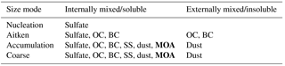
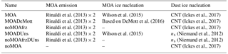
Table 1List of aerosol species present in each of the seven modes. In bold are tracers added in the current study.
2.1 The aerosol–climate model
Simulations in this study are performed using the aerosol–climate model ECHAM6-HAM2. The main atmospheric component is ECHAM6 (Stevens et al., 2013), except for a two-moment cloud microphysics scheme that is coupled to the aerosol module HAM2 (Lohmann et al., 2007). Aerosols are represented as a superposition of seven lognormal size distributions, representing aerosol populations in four size modes and two different mixing states, except for the nucleation mode (number median radius µm) which only contains sulfate aerosol in the internally mixed/soluble mode. All other size modes (Aitken: 0.005 µm < µm, accumulation: 0.05 µm < µm, coarse: 0.5 µm < ) are divided into an internally mixed/soluble mode in which particles are assumed to contain a fraction of all species present, in particular the soluble sulfate aerosol, and an externally mixed/insoluble mode in which each particle is assumed to contain one species only. Only one size distribution (with one total number concentration, median radius, and standard deviation) is considered per mode, while the contribution of each species is represented by their individual masses, which are traced separately.
Various aerosol processes are explicitly represented as described in Zhang et al. (2012). Changes in recent model updates include the use of the Abdul-Razzak and Ghan (2000) scheme for aerosol activation to form cloud droplets, which is based on Köhler theory, and the use of the Long et al. (2011) sea salt (SS) emission parameterisation with a sea surface temperature dependence applied following Sofiev et al. (2011). Also, anthropogenic emissions are fixed at year 2000 levels in the following simulations and the minimum CDNC is 10 cm−3. In the base version used in the current study, aerosol species considered include sulfate, dust, black carbon (BC), organic carbon (OC), and SS, among which dust is allowed to nucleate ice through immersion freezing, following either Ickes et al. (2017) or Niemand et al. (2012) as opposed to Lohmann and Diehl (2006) in the default model set-up. No other type of heterogeneous ice nucleation is considered. Ice multiplication is also not represented in the current model version, as a previous study has found ECHAM6-HAM2 to be insensitive to inclusion of the Hallett–Mossop process following Levkov et al. (1992) (David Neubauer, personal communication, 2017). The relative importance of the various sources of cloud ice crystals in mixed-phase clouds, however, remains an unconstrained property and can thus vary between models.
In the current study, MOA is implemented as an additional species in the internally mixed accumulation and coarse modes, as shown in Table 1 which lists the species present in each of the seven aerosol modes. Aitken-mode MOA is not considered as our model does not consider sea spray production in that size mode. MOA is allowed to nucleate ice through immersion freezing, as described in the following section.
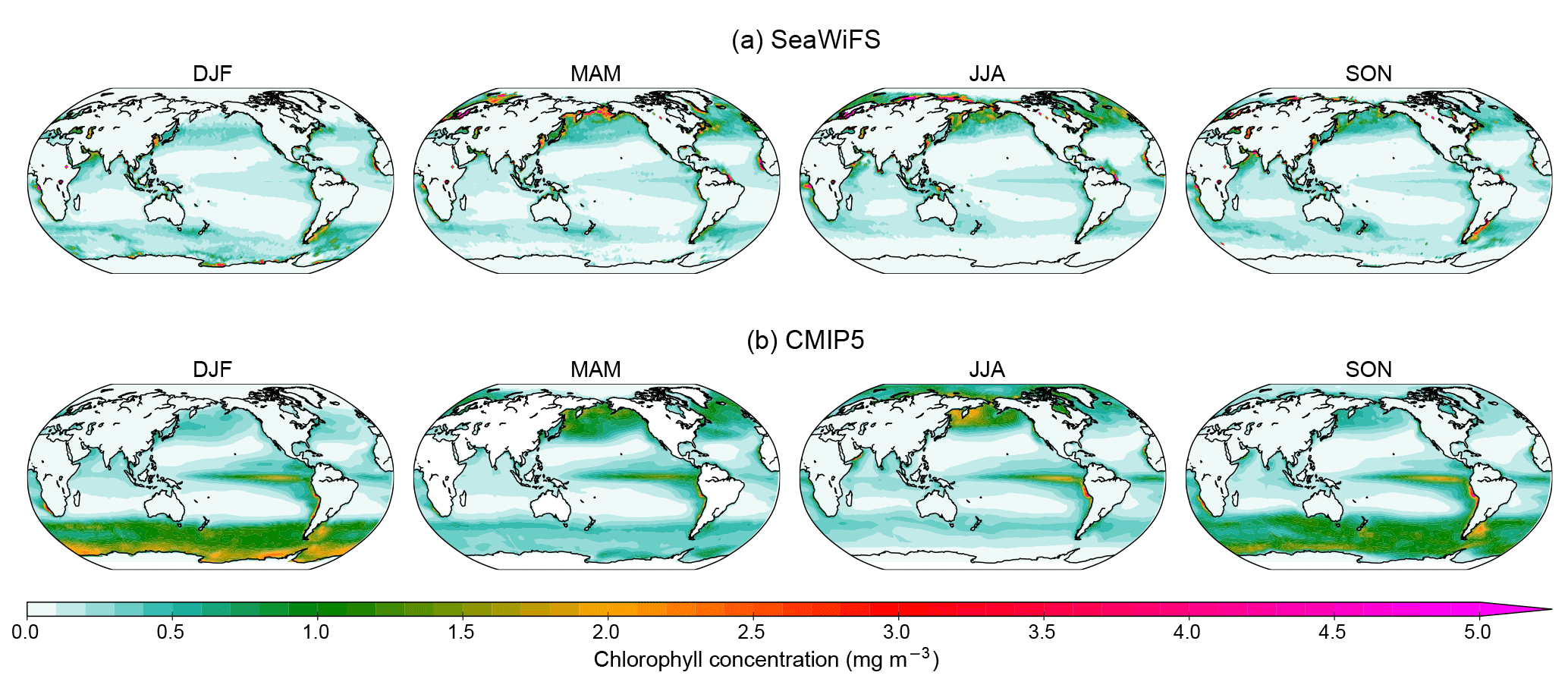
Figure 1Maps of seasonal mean chlorophyll concentrations used as input files for the nudged simulations. The top row shows maps from the SeaWiFS satellite observational dataset from March 2003 to May 2009, and the bottom row shows the mean from CMIP5 historical simulations for the years 2000–2005.
2.2 MOA implementation
2.2.1 Emission of MOA
MOA emission is calculated online and depends on the SS emission, such that the total sea spray emitted is the sum of the two (i.e. sea spray is the combination of SS and MOA), with the organic mass fraction (OMF) defined as . SS is emitted following Long et al. (2011) and remains independent of the MOA emission for all cases except where specified. MOA is then emitted additionally as
The only exception is when MOA is emitted following Long et al. (2011), in which case the SS emission is reduced due to partitioning of some of the emitted mass into MOA. The density of MOA is set to be 1000 kg m−3 (Vignati et al., 2010), with radiative properties identical to those of organic carbon and a hygroscopicity parameter κ of zero. Due to the lack of measurement data, the latter two properties are chosen for simplicity and, for the last case, consistency with other potential INP candidates such as dust particles. While sensitivity to the chosen radiative properties of MOA has yet to be investigated, a previous study by Gantt et al. (2012) has not shown a strong dependence of the results on the chosen hygroscopicity parameter.
No additional number flux due to MOA is considered, as we assume it to be always internally mixed with SS during emission. This is treated differently in different studies, with most emitting MOA as an internal mixture with SS (Long et al., 2011; Vergara-Temprado et al., 2017) while studies by Meskhidze et al. (2011) and Gantt et al. (2012) have noted a stronger impact of MOA on the modelled CDNC when they are assumed to be externally mixed during emission (that is, with an additional number flux but still emitted into internally mixed modes). Unfortunately, no measurement data are available to quantify such potential externally mixed number flux nor the division between internally and externally mixed emissions. Should some of the MOA be emitted separately from SS, they would be part of the externally mixed/insoluble mode in our model. However, as we are interested in the immersion freezing property of MOA, which requires immersion of the aerosol in a cloud droplet that can only occur for soluble/internally mixed particles, for simplicity, we emit all of the MOA into the internally mixed mode directly in order to give an upper estimate of the potential impact of MOA as INP.
Various OMF parameterisations are available in the literature (Burrows et al., 2014; Gantt et al., 2011; Rinaldi et al., 2013; Vergara-Temprado et al., 2017; Vignati et al., 2010), which produce a wide range of MOA fluxes when applied to the global scale, as was also shown in Meskhidze et al. (2011) and Lapina et al. (2011). A measure of marine biological activity is often used in these parameterisations, while some also consider a negative dependence on the near-surface wind speed based on the argument of oceanic mixing leading to a reduction in surface organic enrichment. The performance of each parameterisation is thus also highly dependent on the model wind speeds and choice of representation of the marine biological activity, in addition to the model's SS emission.
In this study, only ocean surface chlorophyll is used to represent the marine biological activity. Despite ongoing debate on the validity of chlorophyll as a proxy for the organic fraction in emitted sea spray, it has been shown that there is currently no better alternative for global coverage and available data (O'Dowd et al., 2015; Rinaldi et al., 2013). Instead, we address the dependence on ocean biological activity data by using two different sources of chlorophyll datasets. In most simulations, multi-year monthly mean level 3 observational data from the Sea-viewing Wide Field-of-view Sensor (Hu et al., 2012) were fed into the model. Free simulations, as will be described later in Sect. 2.3, use the full 12 years of available observational data from 1998 to 2010, while for the nudged simulations, a subset corresponding to the nudged period from March 2003 to May 2009 is used. The two choices of averaging time periods result in only very slight, localised differences in the chlorophyll concentrations (not shown). Such satellite-based observations, however, have a limited coverage in the polar regions in the winter hemisphere that can create a data void as far equatorward as 50∘ (though in the less biologically active winter hemisphere). Also, in light of the possibility to accommodate pre-industrial and future simulations, a sensitivity study is performed using chlorophyll concentration data from the CMIP5 multi-model ensemble outputs (Taylor et al., 2012). Monthly mean chlorophyll maps were created using results from the last 6 years (2000–2005) of the Earth system model (ESM) historical simulations, from which only eight models contain chlorophyll data, as listed in Table B1 in the Appendix. A comparison of the two sets of maps is shown in Fig. 1. Notable deviations of the modelled data from observational means include the lack of peak values near coastlines, which could be due to unresolved coastal processes, coarse model resolution, and averaging across models and/or errors in observations near coastlines; a more widespread coverage of medium concentrations in the high-latitude regions of the spring–summer hemisphere, especially over the Southern Ocean; and persistent local peak concentration in the equatorial upwelling region off the west coast of South America. The impact of such differences is discussed in the results.
Offline calculations were performed to compare the various OMF parameterisations when applied to our model to long-term observations at Amsterdam Island in the southern Indian Ocean (Sciare et al., 2009) and Mace Head in Ireland (Rinaldi et al., 2013), as described in Appendix A. The Rinaldi et al. (2013) parameterisation, which has a maximum OMF set to 78 %, was found to outperform others at both stations when applied to our model. Thus, despite the circular logic of the parameterisation having been derived by using the exact same Mace Head data which we used for validation, the Rinaldi et al. (2013) parameterisation is chosen for our control set-up. This does not, however, guarantee the most realistic emission rate when applied at the global scale. More long-term measurements from different parts of the globe would be required for a better validation of the model simulations.
MOA is emitted into the internally mixed accumulation mode and allowed to grow through coagulation and condensation of sulfate into the coarse mode. This is consistent with the Rinaldi et al. (2013) OMF parameterisation, which is based on observations of submicron emissions. Previous studies have noted a difference in the organic fraction of accumulation- and coarse-mode sea spray, with a higher fraction in the smaller size mode (Facchini et al., 2008). Thus, it would not be appropriate to extrapolate the emission parameterisation to coarse-mode particles, and emission of MOA in the coarse mode is not considered in our simulations.
2.2.2 Heterogeneous ice nucleation of MOA
Quantification of the ice nucleation ability of MOA is still a topic of active research. Currently, only one published parameterisation is available in the literature, namely that of MOA immersion freezing from Wilson et al. (2015). This is an empirical fit to droplet freezing measurements performed using samples collected from the marine microlayer, which gives a purely temperature-dependent parameterisation for the number of INPs per mass of total organic carbon. It should be noted, however, that this parameterisation is developed based on sea surface microlayer samples, which does not necessary reflect the concentration of INPs in the MOA that actually gets aerosolised and emitted into the atmosphere (McCluskey et al., 2017). To convert from the number of INPs per mass of total organic carbon to that per mass of total organic matter, division by a conversion factor of 1.9 is applied. This value lies at the lower end of the range of factors recommended by Turpin and Lim (2001) for non-urban cites, and is chosen since we are only considering water insoluble organics, which are associated with lower carbon-to-molecule conversion in their study. Subsequent publications which investigated airborne sea spray aerosol in the field and produced in laboratory settings (DeMott et al., 2016; McCluskey et al., 2017) have, however, indicated lower ice nucleation efficiencies than that described by Wilson et al. (2015). Therefore, a sensitivity study is also performed by producing a fit to data published in DeMott et al. (2016). Both parameterisations are extrapolated to cover the entire temperature range relevant for mixed-phase clouds (−35 to 0 ∘C in ECHAM6-HAM2). The former is applied to accumulation- and coarse-mode MOA, while the latter, which is a fit representing the ice activity of the total sea spray, is applied to the sum of MOA and SS in the two size modes. For comparison, the parameterisations are plotted together with the ns-based parameterisation of Niemand et al. (2012) for dust aerosol in Fig. 2. Weaker ice activity of MOA compared to dust aerosol can be noted, but MOA could still be important in more remote regions where dust concentrations are low.
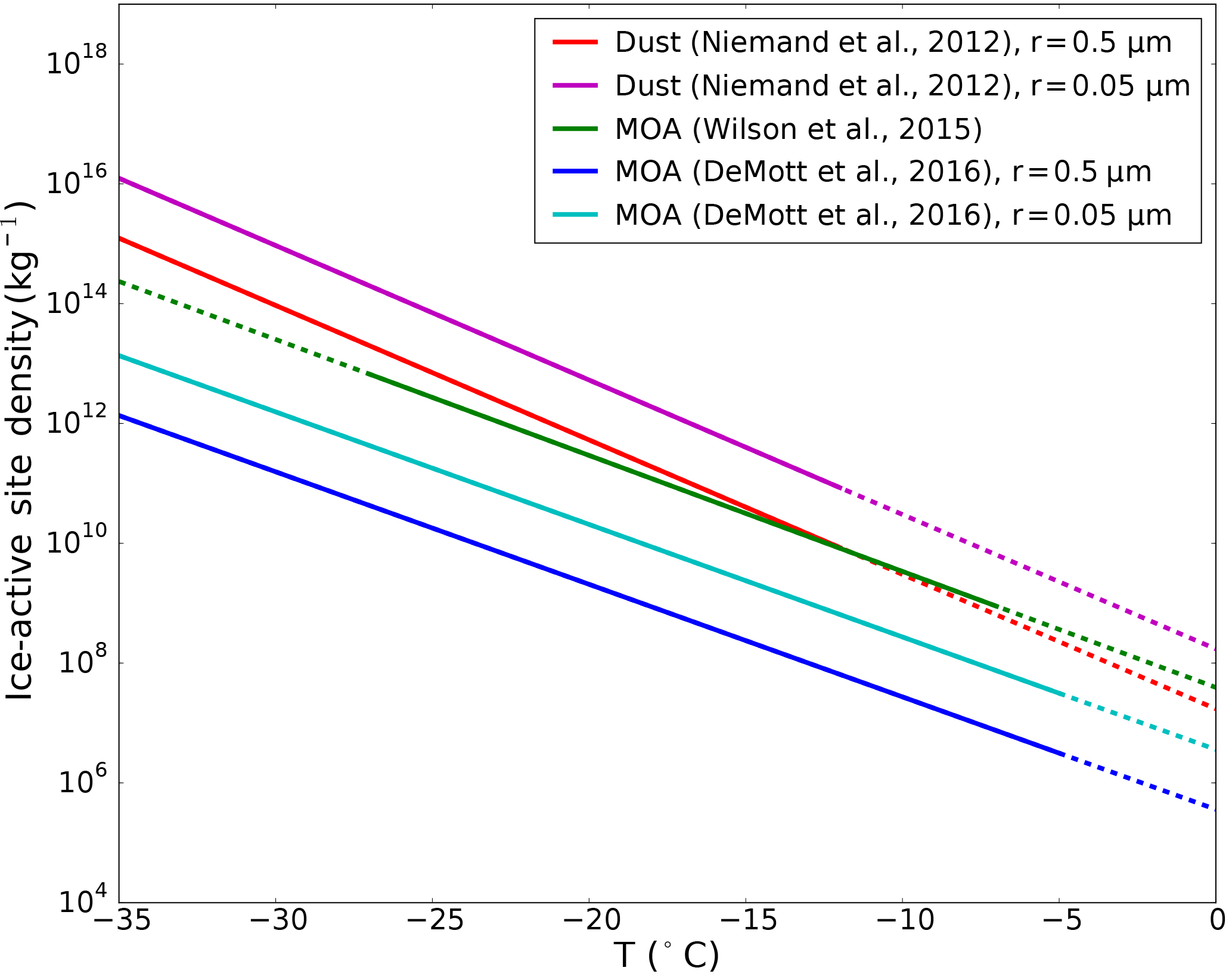
Figure 2 Ice-active site density per unit mass (nm) of the Wilson et al. (2015) parameterisation and of the fit to the DeMott et al. (2016) data, for marine aerosol, as well as the Niemand et al. (2012) parameterisation for dust aerosol. The Wilson et al. (2015) parameterisation is converted from INP number per total organic carbon mass to INP number per MOA mass by dividing by the conversion factor of 1.9. The DeMott et al. (2016) fit and Niemand et al. (2012) parameterisation are converted from the original representation of ice-active site density per unit surface area (ns) by division by their respective density and multiplication by the spherical surface-to-volume ratio using the two extremes in accumulation-mode median radius in our model. The inverse dependence of the ratio on the radius induces higher ice activity of the smaller particle when converting from ns to nm. Solid lines represent the range in which the parameterisations are valid, and dotted lines represent temperature ranges where the parameterisations are linearly extrapolated.
The surface active site density (ns) approach described in Connolly et al. (2009) is extended to consider active site density per mass (nm) and applied to calculate a frozen fraction (FF) given the mean particle mass (mMOA) and temperature. This is then multiplied by the number concentration of MOA immersed in cloud droplets (NMOA,imm), such that the number of drops frozen per time step (Nfrozen) is
NMOA,imm is defined as
following Hoose et al. (2008), where VMOA is the total volume of MOA in the mode calculated by dividing the mass by the density, and VTOT is the summed volume of all species in the internally mixed mode. is therefore a surface area fraction which considers that although the species are internally mixed in the mode, not every particle will contain MOA. A surface area fraction is used as this is the relevant property for ice nucleation. NTOT,act is the number of aerosol particles in the internally mixed mode that can be activated to cloud droplets under current conditions, as calculated following Abdul-Razzak and Ghan (2000). This is equal to the actual CDNC only if the cloud cover or liquid water content in the grid box increased from the last time step, and only if the newly activated number is greater than the previous CDNC (Lohmann et al., 2007).
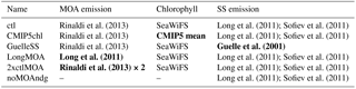
Rinaldi et al. (2013)Long et al. (2011); Sofiev et al. (2011)Rinaldi et al. (2013)Long et al. (2011); Sofiev et al. (2011)Rinaldi et al. (2013)Long et al. (2011); Sofiev et al. (2011)Rinaldi et al. (2013)Long et al. (2011); Sofiev et al. (2011)Long et al. (2011); Sofiev et al. (2011)Table 2List of nudged simulations. In bold are fields which are changed from the control (ctl) set-up. Fields marked with dashes (–) are not relevant for the set-up. “CMIP5chl” uses the chlorophyll concentration from CMIP5 models; “GuelleSS” replaces the SS emission parameterisation by Guelle et al. (2001); “LongMOA” replaces the Rinaldi et al. (2013) MOA emission by Long et al. (2011); for “2xctlMOA”, the control MOA emission is scaled up by two times; and lastly, MOA is not emitted in the “noMOAndg” simulation.
Further pertaining to Eq. (2), the mean mass of MOA in the size mode (mMOA) is obtained by dividing the total mass of MOA in the mode by the total number scaled by the surface area fraction as defined above, and nm,MOA is the temperature-dependent number of active sites per mass, calculated using the Wilson et al. (2015) parameterisation. A slight modification is required for the fit to data from DeMott et al. (2016), which expresses the number of active sites per surface area of total sea spray instead of per mass of MOA. The surface area fraction therefore becomes , and the mean surface area of sea spray per particle is defined as
where is the median radius of all particles in the mode and σ is the standard deviation of the lognormal distribution, which is a size-mode-dependent constant. The smean is then multiplied by ns in the calculation for FF.
One problem with the above method of determining heterogeneous ice nucleation is that, in ECHAM6-HAM2, aerosol particles are not removed due to activation. Rather, in-cloud wet removal only occurs due to precipitation in the form of rain or snow. This leads to possible repeat freezing of the same aerosol across time steps. Indeed, the active site density approach of Connolly et al. (2009) represents the integrated number of ice crystals that can be frozen when the temperature drops from 0 ∘C to the current temperature, which would overestimate freezing if the full range of the temperature drop from 0 ∘C is assumed at each time step. One method to address this is to subtract the ice crystal number concentration (ICNC) from the previous time step from the newly nucleated number, such that only when the latter is greater than the former, does ICNC change due to heterogeneous freezing. This method has the drawback that it assumes that all ice crystals in the mixed-phase temperature range are produced through heterogeneous nucleation. In fact, the largest contributor to mixed-phase ICNC in our model has been found to be sedimentation from cirrus clouds, which can lead to suppression of contributions from heterogenous freezing (Ickes et al., 2018). Thus, in the case that the above method does not lead to an increase in ICNC, a second method is applied where nfrozen calculated using the previous time step's temperature is subtracted from that calculated using the current temperature, such that new ice crystals are produced if the temperature decreased since the last time step. This second method, in turn, does not consider transport of aerosol or changes in moisture between time steps and does not have a memory beyond the previous time step. A combination of both methods is therefore applied to achieve a best estimate of the immersion freezing rate.
Rinaldi et al. (2013)Wilson et al. (2015)(Ickes et al., 2017)Rinaldi et al. (2013)DeMott et al. (2016)(Ickes et al., 2017)Rinaldi et al. (2013)(Ickes et al., 2017)Rinaldi et al. (2013)Wilson et al. (2015)(Niemand et al., 2012)Rinaldi et al. (2013)(Niemand et al., 2012)(Ickes et al., 2017)Table 3List of 10-year free-running simulations. Fields marked with dashes (–) are not relevant for the set-up. “MOA” refers to the control free-running simulation where the Rinaldi et al. (2013) MOA emission is scaled up by two times; “MOADeMott” refers to a simulation where immersion freezing by MOA is replaced by the fit to the DeMott et al. (2016) data for total sea spray; “noMOAfrz” refers to a simulation where MOA is emitted but not acting as INP; “MOADUns” is the same as “MOA” but with the dust freezing parameterisation replaced by the ns scheme following Niemand et al. (2012); “noMOAfrzDUns” is the same as “noMOAfrz” except with a different dust freezing parameterisation; and lastly, “noMOA” is a free-running simulation where MOA is not emitted. CNT indicates classical nucleation theory.
2.3 Simulations
Summarised in Table 2 is a range of sensitivity runs nudged to the same meteorology from March 2002 to May 2009 in order to investigate the impact of different set-ups on the MOA distribution while minimising influences from internal variability. The nudging period is chosen to correspond to the maximum period covered by the MOA concentration measurements performed at the two observational sites, described in Sect. 2.4. As mentioned previously, sensitivity to the chlorophyll concentration is investigated by replacing the SeaWiFS observations with the CMIP5 model mean outputs, while sensitivity to the SS emission is studied by using two different parameterisation schemes. Aside from the default set-up, the Guelle et al. (2001) parameterisation, which was the default SS emission set-up in a previous version of ECHAM6-HAM2 and has a much higher emission rate, is also tested.
In most simulations, the Rinaldi et al. (2013) parameterisation for OMF is used, for it was found to fit best to observations when calculated offline using ECHAM6-HAM2 outputs as mentioned in Sect. 2.2.1 and shown in the Appendix. This type of offline calculations, however, does not allow for proper consideration of particle size dependence, which is included in various size-resolved parameterisation schemes (Gantt et al., 2011; Long et al., 2011). Thus, an additional sensitivity study is performed by using the size-resolved MOA emission parameterisation from Long et al. (2011), which also provides a consistent emission scheme for both SS particles and MOA. In the control set-up and the simulations with the same SS emission scheme, the total sea spray according to the Long et al. (2011) parameterisation, which includes both SS and organic matter, is emitted as SS. MOA mass is then emitted additionally and separately while the SS emission is kept untouched. To be consistent with the original intention of the parameterisation, when both MOA and SS are emitted following Long et al. (2011), the total sea spray is divided between SS and MOA components. This therefore leads to decreases in the SS emission rates when compared to the control simulation.
Lastly, an additional simulation is performed where the MOA emission following Rinaldi et al. (2013) is doubled, and another one where MOA is not emitted at all. The rationale behind these simulations will be shown and discussed in Sect. 3.2 and 3.4.3.
Following the nudged runs, six free-running sensitivity simulations are performed as listed in Table 3. The MOA emission set-up follows the “2xctlMOA” simulation, and is chosen based on the nudged run which best compares to observations, as discussed in Sect. 3.2. Each set-up is run for 10 years (plus 3 months of spin up) with fixed year-to-year external forcing, and a 10-year mean is used during analysis to account for internal variability. As the goal of these free simulations is to investigate the impact of ice nucleation by MOA and its climate feedback, focus is placed on the ice nucleation parameterisations.
MOA ice nucleation rates are studied by using the Wilson et al. (2015) parameterisation and a fit to data from DeMott et al. (2016), which has an ice-active surface site density that is around 2 orders of magnitude lower when converted to the same units. Two different immersion freezing parameterisations for dust, which is the only other heterogeneous freezing candidate in this study, are also tested. Control simulations are performed using a physically based classical nucleation theory (CNT) single-α parameterisation described in Ickes et al. (2017). Properties of montmorillonite as the ice nucleating dust type and an ice nucleation time integration of the first 10 s of each time step are chosen. Another set of simulations is done with the Niemand et al. (2012) ice-active surface site density (ns)-based freezing parameterisation for Saharan dust, which provides a more straightforward comparison to the ice-active site density parameterisation of MOA. The ns parameterisation is extrapolated over the whole mixed-phase temperature regime as is consistent with that of MOA.
Table 4Annual global mean MOA and SS emissions and burdens from nudged simulations. The ratio of MOA to SS emission rates (MOA ∕ SS emission) is a global area-weighted average of the ratio calculated at individual grid boxes. Note that MOA is only emitted in the accumulation mode, while SS is emitted in both accumulation and coarse modes. In the “2xctlMOA” and “CMIP5chl” simulations, slightly different MOA emission properties are considered as explained in Table 2; for “GuelleSS”, a different SS emission is used; and lastly for “LongMOA”, changes are present in both the MOA and SS emissions when compared to the “ctl” run.
Two simulations are done where MOA is emitted but not allowed to nucleate ice, each with a different dust freezing parameterisation (CNT vs. ns), and finally one simulation is set up where MOA is not emitted in the model at all. Analyses of results from all of the above-mentioned simulations are discussed in Sect. 3.
2.4 Comparison to observations
Very limited long-term observations of MOA are available for validation of the model results. The two main sites with available data are Mace Head in Ireland and Amsterdam Island in the southern Indian Ocean. Measured water insoluble organic carbon (WIOC) concentrations from Mace Head spans the time period of 2002–2009 (Rinaldi et al., 2013), while that from Amsterdam Island covers the years 2003–2007 (Sciare et al., 2009). For comparison with observations, model simulations nudged towards the meteorology of the respective measurement periods are used. The measured WIOC concentration is converted to WIOM (i.e. MOA) by multiplying by 1.9 as discussed in Sect. 2.2.2. Due to the limited spatial coverage of satellite-observed chlorophyll concentrations over single months, multi-year monthly mean chlorophyll measurements from SeaWiFS over the time period from March 2002 to May 2009 are used repeatedly for all simulation years. Should the dependence of MOA emissions on chlorophyll concentrations be strong in reality and the chlorophyll concentrations be highly variable from year to year, this will cause biases and inconsistencies in the modelled concentrations when compared to observations. Results from the comparisons are shown in Sect. 3.2.
3.1 Distribution of MOA concentrations
A summary of MOA and SS annual emissions and global burdens from the various simulations is shown in Table 4. A dependence on both the choice of chlorophyll concentration data and the SS emission scheme can be observed, as expected. Notably, a rough doubling of the MOA burden resulted from the doubling of the Rinaldi et al. (2013) MOA flux, indicating a linear dependence of MOA burden on the emission rate. The same cannot be said, however, when the emission parameterisations are changed (for instance, when comparing the “ctl” simulation with “GuelleSS”), which resulted in changes in the spatial distribution of emitted MOA and thus diverging changes in emission and burden.
All emission rates are roughly in line with other quotes in the literature, which consider varying degrees of size resolution (Langmann et al., 2008; Long et al., 2011; Spracklen et al., 2008) and span a wide range of around 5 to 55 Tg y−1 of organic matter. While studies that emit MOA in all size modes and consider both primary and secondary sources can obtain MOA fluxes of over 140 Tg y−1 (Roelofs, 2008), most studies quote emission rates of less than 20 Tg y−1, especially in the submicron size mode (Gantt et al., 2011; Lapina et al., 2011; Vignati et al., 2010). On the global annual average, the mass emission of submicron primary MOA is less than 3.2 % of the SS mass emission in all our simulation set-ups.
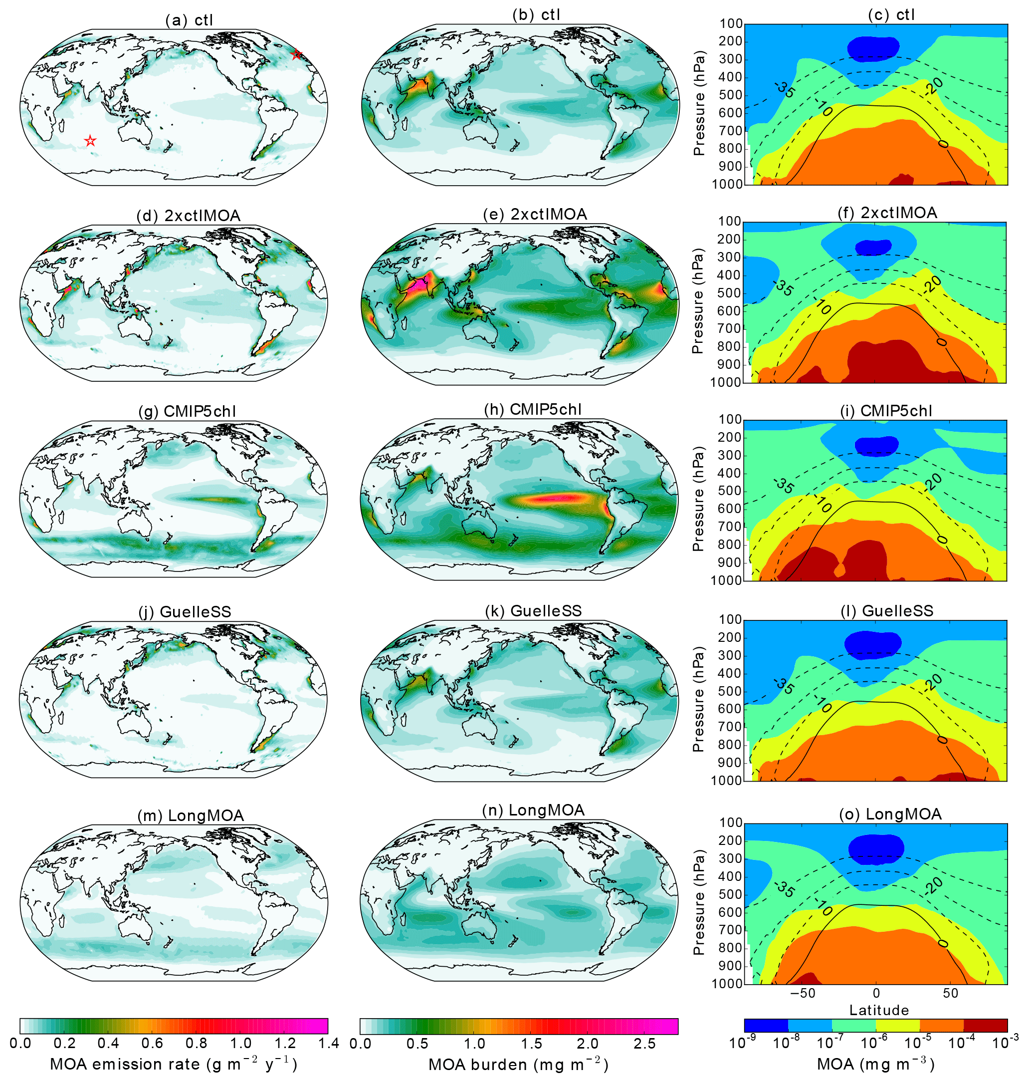
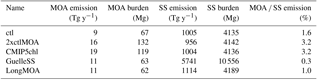
Figure 3Multi-annual mean emissions (a, d, g, j, m), burdens (b, e, h, k, n), and zonal mean cross sections (c, f, i, l, o) of MOA from the various nudged simulations described in Table 2 for the period from March 2002 to May 2009. Contour lines in the zonal mean plots are zonal mean isotherms in ∘C in the mixed-phase temperature range. Red stars in panel (a) indicate locations of Mace Head in the Northern Hemisphere and Amsterdam Island in the Southern Hemisphere, where long-term observations of MOA are available.
Figure 4Monthly mean observed MOA concentrations at Amsterdam Island (a) and Mace Head (b) compared to model simulated outputs as described in Table 2. The dotted blue curve (“offline ctl”) corresponds to an offline calculation of MOA concentration based on the same parameterisation as the control case. The shaded area corresponds to ±1 standard deviation of the observed mean for the Amsterdam Island case, while for Mace Head, it corresponds to the 25th to 75th percentiles. In both cases, the bold black line is the observational monthly mean. Note that no measurements are available for Mace Head in December. Model outputs are averaged over the entire nudging period (March 2002 to May 2009) for comparisons to observations at Mace Head, and averaged over the period of May 2003 to November 2007 for Amsterdam Island, corresponding to the measurement periods.
Annual mean global emission distributions and zonal mean cross sections of the mass concentration are shown in Fig. 3. Using the Rinaldi et al. (2013) parameterisation (all but “LongMOA”), the spatial pattern of MOA emission largely follows that of the chlorophyll concentration. For the simulations using SeaWiFS chlorophyll maps (all but “CMIP5chl”), MOA emissions peak in coastal and equatorial upwelling regions. Due to higher surface wind speeds, a lower emission rate is found in mid-to-high-latitude open ocean regions despite having chlorophyll concentrations comparable to the tropics. Notably, and contrary to expectations based on previous literature (Burrows et al., 2013; Vergara-Temprado et al., 2017; Yun and Penner, 2013), we do not obtain a high concentration of MOA in the Southern Ocean with the Rinaldi et al. (2013) emission, likely also due to the higher wind speeds and moderate chlorophyll concentrations (when using SeaWiFS maps) in these regions. When using CMIP5 mean chlorophyll concentrations, emissions from coastal upwelling regions are reduced, while those from the equatorial upwelling become more pronounced. Much higher MOA emission rates can also be found in mid-to-high-latitude open waters and the Southern Ocean (mainly occurring during the respective hemispheric summer months), as was observed in the chlorophyll concentrations (Fig. 1). An anomalously high emission rate of MOA off the coast of the Arabian Peninsula in boreal summer, observable even in the annual mean in all simulations, is mostly due to the southwest monsoon-associated ocean upwelling and particularly strong SS fluxes. The annual mean signal is weaker in the “LongMOA” simulation, which exhibits a weaker dependence on the wind speed and chlorophyll concentration. This leads to peak MOA emissions off the coast of the Arabian Peninsula only during boreal summer, while relatively high emission rates are also present during boreal autumn and winter in the other simulations, corresponding to the chlorophyll map. The secondary peak in ocean productivity during winter months is associated with deep water mixing caused by colder air blowing over the water surface during the northeast monsoon season (Mann and Lazier, 2005; Wiggert et al., 2000).
The annual mean MOA burden mostly mirrors the emission pattern, with notable accumulations over source regions that are subject to limited precipitation washout. The peak burden in the equatorial South Pacific found in all simulations, for instance, can be associated with the dry zone related to the South Pacific convergence zone that is largely caused by orographically induced subsidence (Takahashi and Battisti, 2007), as well as contributions from subsiding branches of the Hadley and Walker circulations. On the other hand, high emission rates in the northern North Pacific and North Atlantic oceans as well as along the Southern Ocean in the “LongMOA” simulation are not reflected in the annual mean burden, due to washout along the storm tracks.
In the zonal mean cross section, MOA mass is mainly concentrated in the lower altitudes below 700 hPa, and is in general not transported very high up into the atmosphere, as can be expected since MOA is mainly emitted from relatively calm waters. Despite this, non-negligible amounts of MOA still reach mixed-phase temperatures, especially in subpolar regions. All simulations produced similar patterns, with some having a more poleward extent of higher MOA concentrations than others, depending on the emission rates.
3.2 Comparison of MOA concentrations to the observed annual cycle
A comparison of the monthly mean MOA concentrations simulated using the various nudged set-ups listed in Table 2 to the observations at Amsterdam Island and Mace Head is shown in Fig. 4. Notably, the offline-calculated MOA concentration using the same set-up as the control simulation, which was used for choosing the OMF parameterisation as described in Sect. 2.2.1, is also plotted. It can be observed that even with the same parameterisation set-up, offline calculations yielded a stronger seasonal cycle than online calculations. Possible reasons for this deviation include errors in estimating the source regions (since the back trajectories are not explicitly computed using our model), seasonal variations in the aerosol source regions that are not considered in the offline calculations, and a lack of consideration for depletion and sedimentation during transport of MOA to the measurement site. As most MOA emission parameterisations are developed using similar offline methods, it may be worthwhile to note the possible deviation for future parameterisations. Due to the rather low bias of the control simulation, an additional simulation is set up where the control MOA emission using the Rinaldi et al. (2013) OMF parameterisation is increased by a factor of 2 (green curve in Fig. 4), and a better agreement to observations is obtained, despite a rather high bias at Mace Head in March and a low bias in January at Amsterdam Island. This increased emission is thus used as the standard set-up for all subsequent free-running simulations.

Figure 5Seasonal and zonal mean freezing rates due to MOA and dust aerosol during freezing occurrence. Contour lines denote the frequency with which freezing occurs in %. All plots are averages from the 10-year free-running simulations. Only rates where the freezing occurs more often than 0.1 % of the time are plotted.
In examining other simulations with various SS or MOA emission set-ups, we found a general and consistent underestimation of MOA concentrations at both stations. One exception is the simulation using the Guelle et al. (2001) SS parameterisation, which produced reasonable MOA concentrations at Mace Head and hit the lower range of observations at Amsterdam Island except in the first 4 months of the year. The control simulation underestimated MOA concentrations at both stations. Simulation with MOA emitted following the size-resolved Long et al. (2011) parameterisation, on the other hand, was not able to reproduce the annual cycle of MOA concentrations well, despite yielding higher concentrations at Amsterdam Island. By replacing the SeaWiFS chlorophyll observations with CMIP5 mean modelled outputs, a significant underestimation of MOA concentrations resulted at Mace Head, while for Amsterdam Island, a relatively good fit to the observed annual cycle of MOA concentration is produced except for the months of October to December, where the CMIP5 models produced a widespread peak in chlorophyll concentrations in the Southern Ocean not observed by the satellite. This led to the decision to not use the CMIP5 mean chlorophyll map for the longer-term simulations, and points to the need for more MOA measurement sites and improvements in the simulation of chlorophyll concentrations in ocean models, as well as a need for caution in future MOA-related model studies where modelled chlorophyll concentrations need to be used. Notably, however, the “CMIP5chl” simulation is the only simulation which is able to reproduce the strong peak in MOA concentrations during the austral summer months (DJF) at Amsterdam Island, which may point to an underestimation of the multi-year mean SeaWiFS chlorophyll concentrations in these months or to other missing marine organic sources not directly associated with chlorophyll.
3.3 Heterogeneous ice nucleation
Ice nucleation rates due to immersion freezing of MOA and dust aerosol and their respective frequencies of occurrence when applying the various parameterisations are shown in Fig. 5. One clear observation is the at least 3 order of magnitude difference between the peak freezing rates of dust aerosol and MOA. Aside from this, freezing occurs with the same frequency for all active site density schemes (contour lines in Fig. 5). Freezing calculated using this parameterisation approach occurs whenever the environmental condition is conductive for freezing at an ambient temperature between 0 and −35 ∘C, the relevant ice-active aerosol species is present in sufficient amounts (relative to the respective ice activity), and the considerations for refreezing as described in Sect. 2.2.2 are fulfilled. This indicates that, in most cases, MOA and dust aerosol are both present in sufficient amounts, and thus freezing occurs for both species if the environmental factors allow.
Such direct conclusions cannot be drawn from comparison with the CNT results, however. While the CNT-based dust freezing scheme produces a lower freezing occurrence frequency overall and especially in the warmer temperatures compared to MOA (Fig. 5), a similar difference in freezing occurrence frequency can also be noted between the results from the two dust freezing schemes, which points to the parameterisation as the main reason behind the difference. The sharp decrease in freezing occurrence at warmer temperatures following Ickes et al. (2017) when compared to the results using the Niemand et al. (2012) dust parameterisation indicates a faster decrease of the dust ice activity with increasing temperature for the former set-up, which is shown in Fig. 6. Indeed, the FF of 0.5 µm radius particles following Ickes et al. (2017) quickly drops below that following Niemand et al. (2012) at around −31 ∘C, and below that of MOA following Wilson et al. (2015) at around −29 ∘C. At −20 ∘C, even with the maximum monthly mean immersed dust concentration on the order of 100 cm−3, only around 10 droplets per cubic kilometre of air will freeze. Without sufficiently large dust particles and/or sufficiently high number concentrations, the Ickes et al. (2017) CNT parameterisation will thus not lead to much ice nucleation occurrence in the warmer mixed-phase temperatures. Interestingly, a surface active site density approach for montmorillonite (consistent in dust type with the CNT parameterisation), which is also compared in Fig. 6, can be noted to have a less steep slope than the CNT approach, though still a faster decrease in FF than that from Niemand et al. (2012). As the Niemand et al. (2012) parameterisation considers a mixture of dust mineral types, this indicates that the difference in freezing rates between the Ickes et al. (2017) CNT parameterisation and the Niemand et al. (2012) parameterisation may be a consequence of both a difference in parameterisation method (CNT vs. ns) and the considered dust type (montmorillonite vs. Saharan dust). A CNT-based parameterisation for MOA cannot be formulated, however, due to the lack of measurement data. It is therefore impossible to conclude how much of the difference in the frequency and regions of occurrence between freezing by MOA and CNT-parameterised dust is related to the different INP species and how much is simply due to differences in the parameterisation approach.
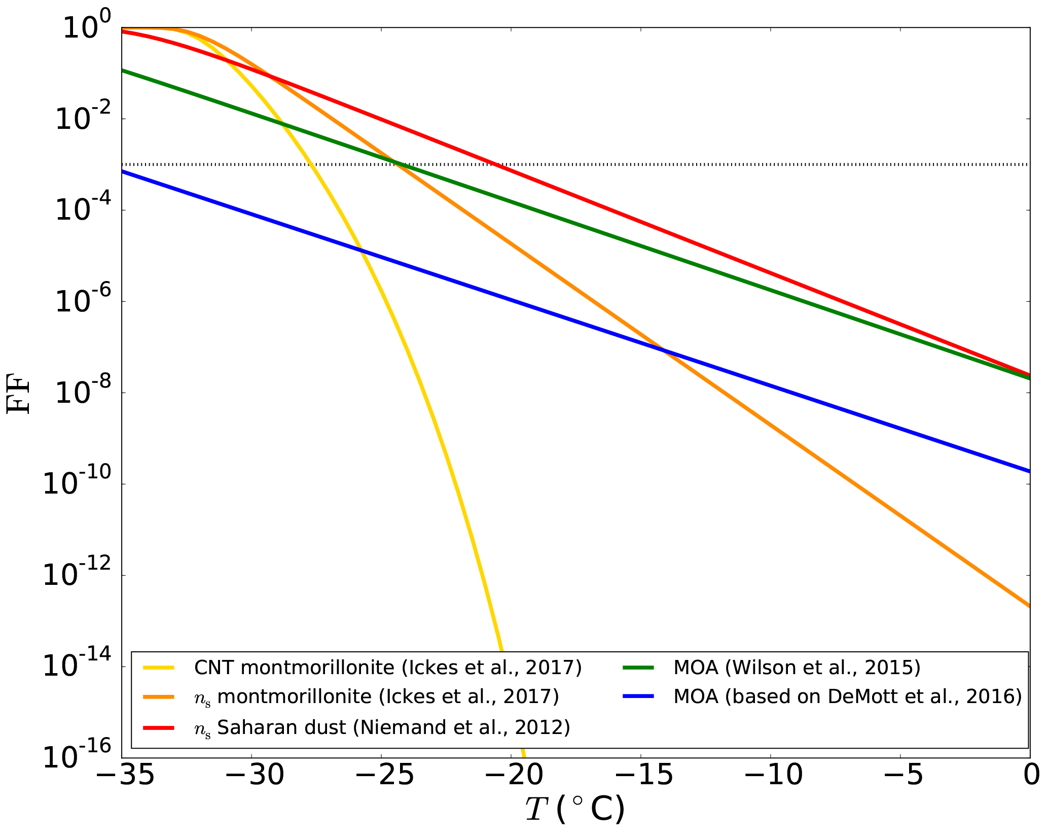
Figure 6Frozen fraction (FF) vs. temperature (T) of the various parameterisations used for dust aerosol (montmorillonite and Saharan dust) and MOA in this study. Spherical aerosol of radius 0.5 µm and an ice nucleation time of 10 s for the CNT method are assumed. In addition to the parameterisations previously discussed in the text, an additional ns-based parameterisation for montmorillonite is also plotted following Ickes et al. (2017). The dotted black line indicates the freezing onset (0.001 FF).
3.3.1 Immersion freezing by dust
Dust freezing rates following CNT (Ickes et al., 2017) and the surface active site density approach using the Niemand et al. (2012) parameterisation show consistent results in the spatial distribution and magnitude of peak values mainly in the colder mixed-phase temperature range. The Niemand et al. (2012) parameterisation, which is extrapolated for temperatures warmer than −12 ∘C, leads to more frequent freezing occurrence, especially notable at warmer temperatures, albeit with significantly lower freezing rates when compared to that in colder regions. This is associated with the differing slopes of the two parameterisations, as discussed in the previous section and shown in Fig. 6. When expressed as the onset freezing temperature, defined as the temperature at which a FF of 0.001 is reached, this translates to −21 ∘C for Niemand et al. (2012) and −28 ∘C for Ickes et al. (2017), assuming spherical aerosol of radius 0.5 µm.
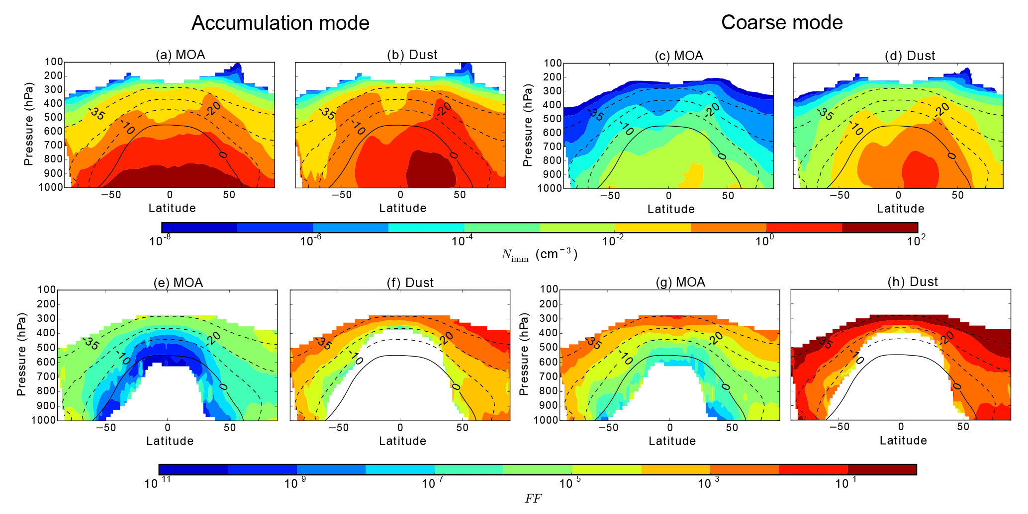
Figure 7Multi-annual, zonal mean number of accumulation-mode (a, b, e, f) and coarse-mode (c, d, g, h) particles immersed in droplets (Nimm; a–d) and the frozen fraction (FF; e–h) for MOA (a, e and c, g) and dust aerosol (b, f and d, h), from the free “MOA” simulation with the Wilson et al. (2015) freezing parameterisation for MOA and CNT for dust. Contour lines denote isotherms in the mixed-phase temperature range. FF is only plotted where the freezing occurs more frequently than 0.1 % of the time.
3.3.2 Immersion freezing by MOA
The MOA freezing rate scales proportionally with the ice-active site density, with freezing rates increasing by around 2 orders of magnitude (depending on the aerosol size) when using the Wilson et al. (2015) parameterisation compared to the DeMott et al. (2016) parameterisation. The freezing onset temperatures of MOA for the same conditions as described above for dust are −36 and −24 ∘C, respectively, for the parameterisation in the “MOADeMott” and “MOA” set-ups.
3.3.3 MOA vs. dust as INP
The immersion freezing rate, as described by Eq. (2), is calculated by multiplication of the number of aerosol particles available for freezing, which depends on the abundance and distribution of the aerosol as defined in Eq. (3), and the FF, which depends on the property of the aerosol (size- and temperature-dependent ice activity). A decomposition of these two components for MOA and dust is shown in Fig. 7. Here, it can be noted that the number concentrations of immersed MOA and dust aerosol span similar orders of magnitude in the accumulation mode, while in the coarse mode the abundance of dust aerosol can be up to 2 orders of magnitude larger. The FF, on the other hand, shows a more uniform 2–3 order of magnitude difference between dust aerosol and MOA regardless of the size mode. Thus, the temperature-dependent aerosol ice activity can be attributed as the main controlling factor behind the number concentration of nucleated ice crystals as compared to the availability of the particles. This can also be concluded by noting the small change in MOA freezing rates when different SS emission parameterisations or chlorophyll maps are used (not shown). Nonetheless, the larger amount of MOA near the surface can contribute to higher ice nucleation rates in polar near-surface regions despite the warmer temperature.
So far, only seasonal or annual mean freezing rates have been shown. However, monthly mean dust concentrations in the air could be dominated by episodic dust events which would mask potential contributions from MOA during periods of low dust concentrations. Thus, online diagnostics of the time frequency when the freezing rate of MOA is greater than that of the dust aerosol is performed for cloudy mixed-phase grids containing supercooled droplets and shown in Fig. 8. Different combinations of MOA and dust freezing parameterisations are investigated.
When comparing the diagnostic results with varying set-ups of freezing by MOA, no systematic differences are present. In particular, no noticeable change in the frequency of occurrence resulted from a 2 order of magnitude decrease in the MOA ice activity, as can be noted from comparison between the “MOA” and the “MOADeMott” simulations. This can be attributed to the similarities between the frequency of MOA freezing occurrence of the two simulations as shown in Fig. 5 (contours).
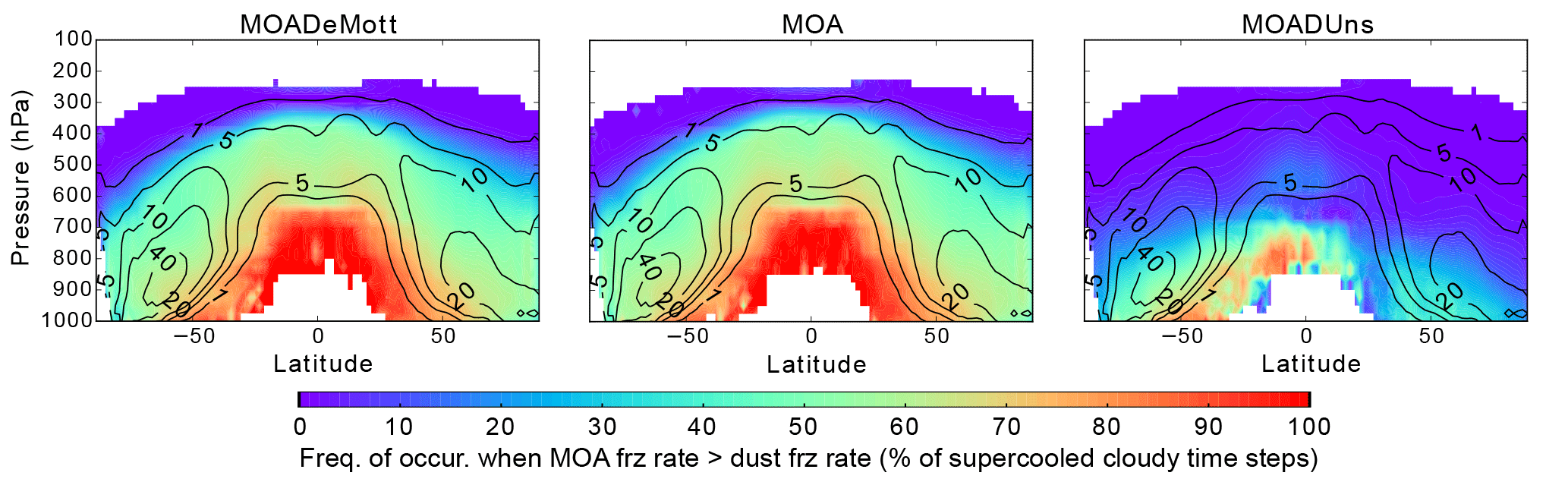
Figure 8The annually and zonally averaged frequency of occurrence when the freezing contribution from MOA is greater than that from dust aerosol, diagnosed only for cloudy grid boxes containing supercooled droplets. Contour lines denote the frequency of occurrence (in %) of the above-mentioned favourable cloudy condition containing liquid droplets in the mixed-phase temperature range. All plots are from the respectively titled 10-year free-running simulations.
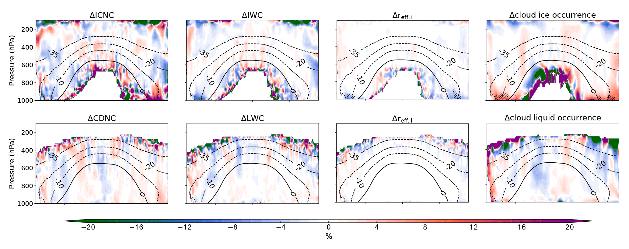
Figure 9Annual and zonal mean relative change (“MOA” minus “noMOAfrz” divided by the mean of the two) in ice crystal number concentration (ICNC), ice water content (IWC), ice crystal effective radius (reff,i), ice cloud occurrence frequency, cloud droplet number concentration (CDNC), liquid water content (LWC), cloud droplet effective radius (reff,l), and liquid cloud occurrence frequency. All values are in-cloud changes (i.e. during liquid/ice cloud occurrence, respectively). Contour lines are zonal mean temperatures in the mixed-phase range in ∘C. Hatched areas indicate statistical significance at the 95 % level following the Wilks (2016) method for controlling the false discovery rate for data with moderate to strong spatial correlations.
While the choice of MOA freezing parameterisation does not have a significant qualitative influence on the result of such diagnostics, that of the dust ice nucleation parameterisation plays a significant role. This is due to the much lower freezing frequency from the CNT-based approach, especially in warmer temperature regimes. When the Wilson et al. (2015) parameterisation for MOA is combined with the Ickes et al. (2017) CNT parameterisation for dust (simulation “MOA”), the contribution from MOA frequently dominates over that from dust aerosol over much of the warmer mixed-phase regions. When the Niemand et al. (2012) ns parameterisation is applied for dust, however, MOA only becomes more important than dust in the warmest mixed-phase regions near the surface in polar regions and in the Southern Hemisphere low altitudes. This difference can be attributed to the different slopes and dust freezing onset between the CNT and ns parameterisations, as noted previously in Sect. 3.3.

Regardless of differences between different freezing parameterisation set-ups, MOA has been found to contribute to more freezing than dust during up to 20 to 70 % of the time in much of the mixed-phase cloud regions when using the Ickes et al. (2017) CNT dust scheme, and up to 60 % near the surface in the Southern Hemisphere when using the Niemand et al. (2012) dust scheme. This is largely comparable to the values found by Vergara-Temprado et al. (2017), who examined the percentage of days when the INP concentration at ambient temperatures from MOA is greater than that from K-feldspar. As their study also uses a ns-based freezing parameterisation for dust, the most straightforward comparison would be with our “MOADUns” simulation, in which case slightly lower freezing contributions from MOA are found in our results. This is especially notable in the Northern Hemisphere and in higher altitudes in the Southern Hemisphere. Possible reasons for this include their choice of only considering freezing by a fraction of the dust (K-feldspar) instead of all dust aerosol in our case, which decreases the availability of dust particles in their study and leads to a more ready scavenging of the dust INP from the atmosphere due to the larger size of feldspar, as noted also by Vergara-Temprado et al. (2017). Additionally, the freezing parameterisations are not extrapolated to all mixed-phase temperatures in their study, and lastly, differences in emission, partitioning, removal, and transport of the aerosol exist between models. It should be noted, however, that both the current work and the study by Vergara-Temprado et al. (2017) only consider MOA in combination with dust aerosol as the sole INP species. Should other INPs active at relatively warm temperatures be included (Vali et al., 1976), the relative importance of MOA may be dampened.
3.4 Impact on clouds and climate
3.4.1 Impact on clouds
INPs can impact clouds through freezing of supercooled liquid droplets and subsequent ice crystal growth at the expense of the remaining liquid drops, leading to glaciation of the cloud. The most direct impact of MOA as an INP would thus be expected in the cloud ice and liquid properties. This is shown in Fig. 9 as the annual mean in-cloud relative difference between one simulation where the expected impact of MOA acting as INP is greatest (“MOA”) and the corresponding simulation where it is not allowed to initiate freezing (“noMOAfrz”). The most statistically significant changes in cloud properties are found near the surface in polar regions, with a decrease in the in-cloud zonal and annual mean ice crystal radius (reff,i) by up to 3 to 9 % and an increase in the cloud ice occurrence frequency by 5 to 28 %.
To investigate the cause for the changes in reff,i and cloud ice occurrence frequency, seasonal mean changes in the cloud ice properties are shown in Fig. 10. Though mostly statistically insignificant following the strict Wilks (2016) criterion, strong relative increases in the cloud ice occurrence frequency, in-cloud ICNC, and to a lesser extent the in-cloud IWC can be observed in the polar regions especially during their respective summer months. A stronger signal can be noted in the Arctic during boreal summer, likely due to the higher temperatures in these regions leading to rare ice occurrences in general and thus stronger relative sensitivity to contributions by MOA.
The observed decrease in reff,i, on the other hand, does not exhibit statistical significance on a seasonal scale (except in the Arctic during boreal autumn). Rather, a consistent but weak decrease in the ice crystal size can be observed near the surface over both polar regions for all seasons. A possible explanation is that since MOA initiates ice crystal formation at relatively warm mixed-phase temperatures closer to the surface, the newly formed ice crystals do not have enough time to grow further. This is particularly notable when compared to ice falling from higher levels, which is also more likely to reach lower levels if the crystal sizes are larger. The newly nucleated ice crystals therefore lead to a lower in-cloud ice crystal radius near the surface.
3.4.2 Impact on the TOA radiative balance
The change in the zonal mean top-of-atmosphere (TOA) radiative balance due to the emission and/or ice activity of MOA in the various free-running set-ups is shown in Fig. 11. When comparing our strongest MOA potential set-up (“MOA”) to one where MOA is not emitted at all (“noMOA”), the TOA net solar radiation decreases by 0.16 W m−2 on the global mean with the added MOA, while the net outgoing terrestrial radiation decreases by 0.03 W m−2, leading to a decrease of 0.13 W m−2 in the net TOA radiation. When decomposing the contribution into that from the emission of MOA (“noMOAfrz”–“noMOA”) and that from MOA acting as INP (“MOA”–“noMOAfrz”), neither process can be ruled out as a contributor to the change. This can include cooling at the surface due to the direct scattering effect of the emitted MOA and that due to the increased aerosol indirect effect on cloud radiative properties induced by MOA acting as INP, as well as further feedbacks triggered by the two processes.
In the shortwave (SW), a statistically significant decrease in the net TOA incoming radiation of around 0.3 W m−2 over Antarctica can be observed in association with the added MOA. Up to a 1.3 W m−2 decrease can also be noted in the Arctic region associated with the freezing of MOA. However, the pattern of change is mostly not consistent across the different set-ups. No consistent pattern north of 50∘ S can be observed in the changes due to MOA acting as INP when the dust ice nucleation parameterisation is changed from Ickes et al. (2017) to Niemand et al. (2012) (i.e. dark blue vs. light blue curves in Fig. 11). Similarly, differences in the MOA ice nucleation parameterisation (i.e. black vs. gray curves in Fig. 11) cause some non-statistically significant changes, especially in the Northern Hemisphere. This is indicative of internal variability of the system and feedback processes which are further examined in the next section.
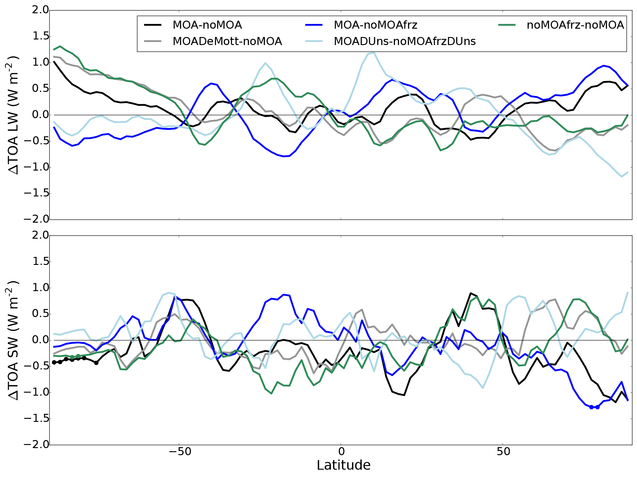
Figure 11Zonal and multi-annual mean change in the top-of-atmosphere (TOA) solar (SW) and terrestrial (LW) radiative balance for the various free-running 10-year simulations. The black and gray curves indicate changes due to both the emission and ice nucleation of MOA, the blue-coloured curves correspond to changes stemming from MOA ice nucleation, and the green curve indicates changes due to the emission of MOA. It should be noted that the outgoing terrestrial radiation is defined to be negative, so a positive change is indicative of less outgoing radiation. Statistically significant changes at the 99 % level are marked with dots on the respective curves.
3.4.3 Impact on dynamics
The changes in the zonal mean aerosol and cloud properties together with the changes in TOA radiative balance due to the emission and ice activity of MOA in the “MOA” set-up are shown in Fig. 12a, d. In particular, the SW aerosol forcing mirrors rather well the increase in aerosol optical depth (AOD, global mean increase of 0.006) at the various latitudes, indicating an expected increase in scattering effect due to the added MOA. On the global mean, the TOA all-sky instantaneous aerosol forcing decreases by 0.069 and 0.008 W m−2 in the SW and LW, respectively, yielding a net decrease of 0.061 W m−2. This does not, however, translate to changes in the TOA radiative balance, which is only significant in the shortwave radiation over the Southern Hemisphere high latitudes, as discussed in Sect. 3.4.2. Rather, the latter signal may be due to internal variability and feedback processes.
To further investigate possible causes for the signal in radiative balance changes over Antarctica, the relevant simulations (“MOA” and “noMOA”) are extended for an additional 10 years and the resulting changes shown in Fig. 12b, e. Notably, while the general pattern of the changes is preserved, the magnitude of the signal is largely diminished in nearly all properties, and no statistical significance remains in the changes in the TOA radiative balance. An exception is the increase in AOD over the Northern Hemisphere tropical latitudes and midlatitudes and the change in SW aerosol forcing, both of which show a stronger signal averaged over the 20-year simulation. Virtually no significance can be found, however, in any of the zonal mean cloud or environmental variables investigated. Therefore, we conclude that MOA emission and MOA acting as INPs do not have significant impacts on the global radiative balance and climate variables.
Lastly, to suppress feedback processes through dynamics, analyses of nudged simulations with otherwise the same set-ups (“2xctlMOA” and “noMOAndg”) are performed where the vorticity and divergence of the flow fields are nudged toward the same meteorology for the two simulations. The changes in the climate and cloud properties are shown in Fig. 12c, f, where it can be noted that any changes in the examined properties are diminished and no significant impact of MOA on the modelled climate can be observed. The pattern of mirrored changes in the AOD and aerosol forcing is, however, consistent with other simulations.
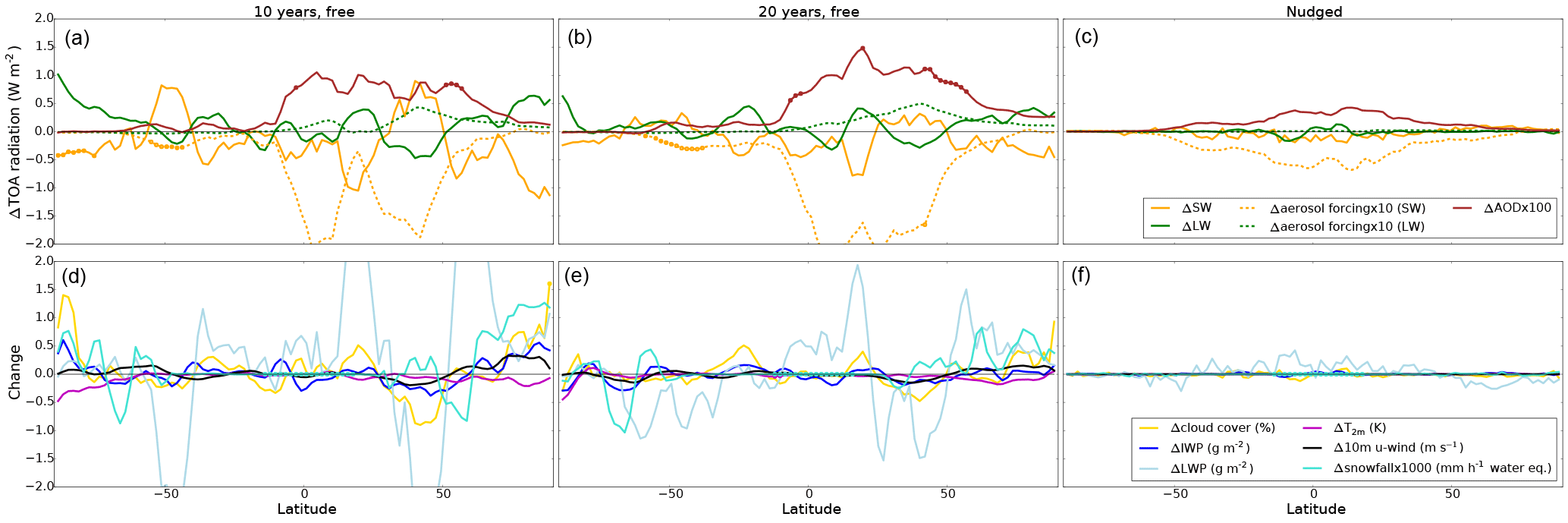
Figure 12(a–c) Zonal, multi-year mean changes (“MOA”–“noMOA”) in the top-of-atmosphere (TOA) solar (SW) and terrestrial (LW) radiation in all-sky conditions, the corresponding changes in aerosol forcing at the TOA scaled up by an order of magnitude, and the change in aerosol optical depth (AOD) at the 550 nm wavelength scaled up by 2 orders of magnitude to fit the same scale on the y axis. (d–f) Zonal, multi-year mean changes in cloud cover, ice water path (IWP), liquid water path (LWP), 2 m temperature (T2 m), 10 m zonal wind (10 m u wind), and water equivalent snowfall rate. Panels (a) and (d) are changes from the 10-year free-running simulations, (b) and (e) are changes from simulations identical to those on the left except they are extended for another 10 years, and (c) and (f) are from the nudged simulations. Small circles on the curves indicate statistical significance at the 99 % level.
In this study, a range of simulations is set up to investigate the emission and distribution of MOA on the global scale. Three different aspects that control the emission rate are tested, namely the SS emission parameterisation, the MOA emission parameterisation, and the chlorophyll map. A weaker dependence on the SS emission parameterisation is found compared to the choice of chlorophyll data and MOA emission parameterisation. In particular, the use of the CMIP5 mean modelled chlorophyll data to replace SeaWiFS observations leads to significant changes in the MOA spatial distributions. A cause for this is the systematic overestimation of total chlorophyll concentrations in the Southern Ocean that is common among global ocean models (Le Quéré et al., 2016). This should be taken into account for future simulations using modelled chlorophyll concentrations. The vertical distribution of MOA, however, is relatively similar between simulations, with the mass mostly concentrated in the lower levels.
Following previous studies proposing MOA as a potentially important INP (Burrows et al., 2013; Vergara-Temprado et al., 2017; Wilson et al., 2015; Yun and Penner, 2013), contributions of MOA to heterogeneous ice nucleation are investigated. When compared to dust aerosol, MOA is found to nucleate 3–4 orders of magnitude fewer ice crystals during freezing occurrence, depending on the choice of parameterisation, due to its weaker ice activity. When compared to the CNT-based dust parameterisation for montmorillonite (Ickes et al., 2017), however, MOA commonly contributes to more freezing of liquid droplets in 50 % of the cases in the mixed-phase temperature range. On the other hand, when applied together with the Niemand et al. (2012) parameterisation for dust aerosol, MOA only contributes to more heterogeneous ice nucleation than dust in the low-altitude regions. This occurs more often in the Southern Hemisphere, where the mass concentration of MOA is higher and where the dust concentration is lower due to the hemispheric dependence of dust emissions that favours the Northern Hemisphere. The difference between the comparisons to the two different dust parameterisations mainly stems from their differing rates of FF decrease with increasing temperature. When expressed in onset freezing temperature, this is 7 ∘C lower for the Ickes et al. (2017) CNT parameterisation compared to −21 ∘C for Niemand et al. (2012), assuming a spherical aerosol radius of 0.5 µm. The onset temperatures then further diverge with lower threshold FFs. The overall importance of MOA as an INP when compared to mineral dust is thus highly dependent on the choice of freezing parameterisations, for both MOA and dust. This points to the need for more measurement data to better constrain the parameterisations, especially at warmer temperatures. Additionally, as the current study disregards potential heterogeneous ice nucleation by other aerosol species aside from MOA and dust aerosol, the relative importance of MOA may be overestimated when compared to the case where other INPs are considered. This would be particularly relevant for INP species that have a high ice activity at warmer temperatures, where MOA is more ice active than dust aerosol in the current study, such as pollen and fungal spore (Dreischmeier et al., 2017; Fröhlich-Nowoisky et al., 2015). The global atmospheric relevance of the various species, however, can also depend on their abundance and various other factors (Hoose et al., 2010), and therefore their impact on the relative importance of MOA as an INP cannot be directly inferred.
Extending the analysis one step further, impacts of MOA on clouds and climate are also investigated in this study. In general, weak to no statistically significant changes in cloud and climate variables are found due to the addition of MOA and due to MOA acting as an INP. More specifically, a decrease in in-cloud reff,i by up to 3 to 9 % and an increase in cloud ice occurrence frequency by 5 to 28 % near the surface over both polar regions can be identified due to MOA initiating ice formation in the presence of supercooled droplets. In the climate variables, any statistically significant change is largely diminished when the simulations are extended to 20 years. This points to the possibility that a 10-year mean is not sufficient to rule out internal variability in high latitudes as the reason behind the observed signals, and has implications for future studies focusing on high-latitude regions where longer simulations may be advised. When dynamical feedbacks are suppressed through nudged simulations, the changes are further diminished. We therefore conclude that any potential impact of the emitted MOA or MOA acting as an INP on the model climate is masked by the internal variability of the model. This can be partly attributed to the weak sensitivity of our model to heterogeneous ice nucleation (due to the dominating contribution of cloud ice from sedimentation of ice crystals originating from cirrus levels; Ickes et al., 2018), as well as to the weak ice activity of MOA when compared to dust.
Data associated with this publication can be found at https://data.iac.ethz.ch/MOAacp/ (Huang, 2018).

Figure A1Comparison of MOA concentrations calculated offline using various OMF parameterisations. Coloured lines indicate offline calculated concentrations assuming the same source regions as the observational datasets; dotted lines of the same colours correspond to the same parameterisations except for the use of source regions from Vergara-Temprado et al. (2017). The black lines and shaded areas are the observational mean and the corresponding variances as described in Fig. 4.
Offline calculated monthly mean MOA concentrations at the two observational sites are shown in Fig. A1 using various OMF parameterisations. Monthly mean modelled 10 m wind speeds and SS concentrations from a nudged simulation without MOA, averaged over the relevant period for each observational site (March 2002 to May 2009 for Mace Head and May 2003 to November 2007 for Amsterdam Island) are used in combination with the mean SeaWiFS observed chlorophyll concentrations from the longer period. Two emission source regions for the aerosol reaching the measurement site are considered for each observational site: one following the region noted in the cited literature with the observational data and the other approximated from Vergara-Temprado et al. (2017). The two differ slightly due to consideration of atmospheric-transport-based different observational and modelled data, but both only serve as an approximation as the transport pattern in ECHAM6-HAM2 would again be different. OMFs are calculated offline for each source region using each OMF parameterisation and the chlorophyll concentrations and wind speeds from the corresponding region, as needed. Observed WIOC is converted to WIOM with a conversion factor of 1.9 as discussed in Sect. 2.2.2. As the OMF parameterisations are valid for the organic fraction during emission, the MOA concentration shortly after emission is approximated by taking the SS concentration in the lowest model level with the derived OMF, following Eq. (1). The MOA concentration for the measurement site is then taken as the average of the concentrations over the entire source region. A schematic of the source regions is shown in Fig. A2.
Notably, the calculated MOA concentration can vary by more than 0.1 µg m−3 with slight shifts in the chosen source region, as can be observed by comparing solid and dotted curves in Fig. A1. When both source regions are considered, the Rinaldi et al. (2013) parameterisation is chosen as the best fit to observations, though with a general slight underestimation. It should be noted, however, that the assessment for the wellness of fit to observations is highly model-dependent. Thus, while suitable for choosing an appropriate OMF parameterisation for this particular model, no generalisations should be drawn with regards to the individual parameterisations when applied to other models. Indeed, each of the OMF parameterisations has been separately validated in their respective studies and found to fit well to observations in its respective set-ups.
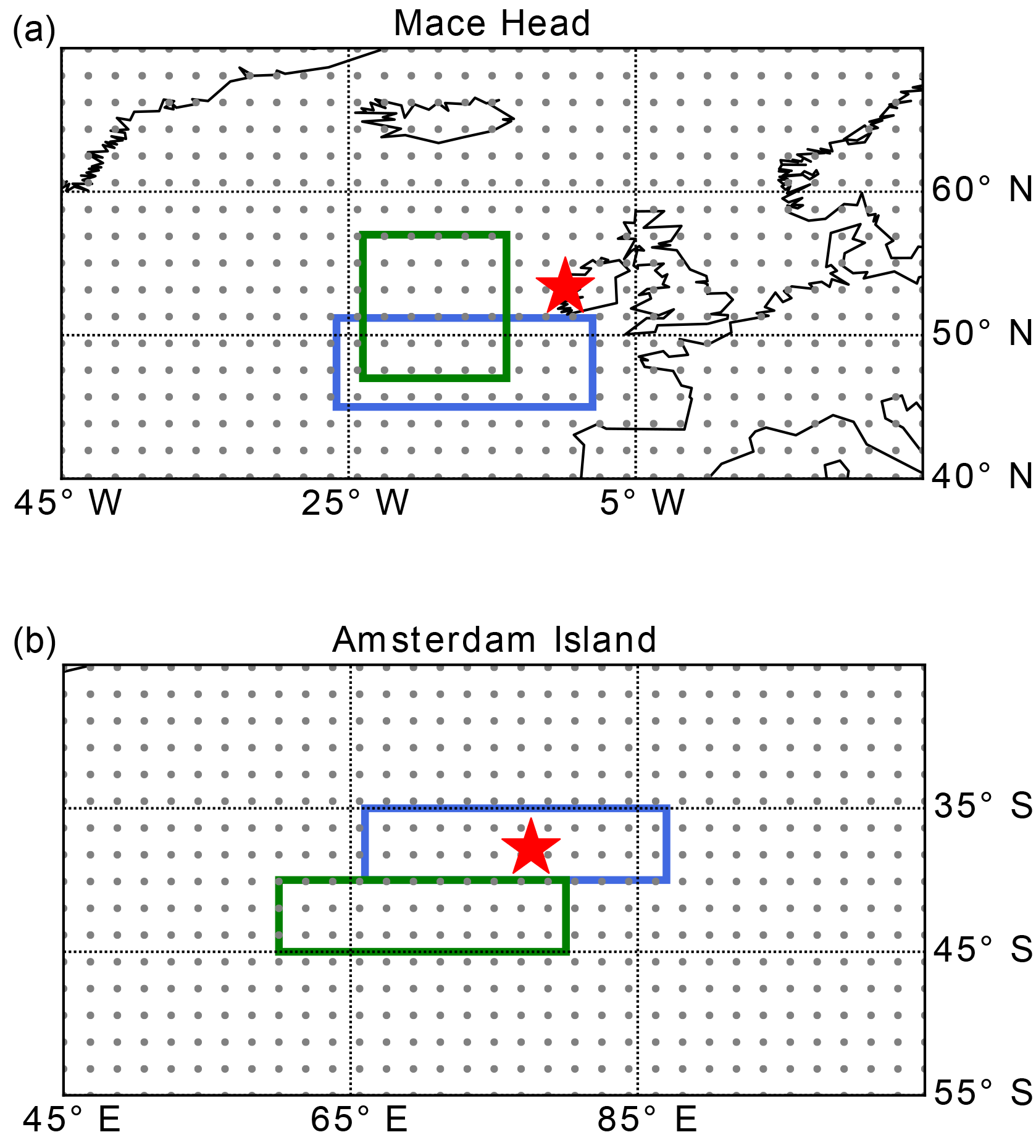
Figure A2Source regions considered in offline calculations of MOA concentrations at Mace Head (a) and Amsterdam Island (b) according to various OMF parameterisations. The area boxed in green is the source region from the relevant publication related to each observational dataset, while that in blue is approximated from Vergara-Temprado et al. (2017). The red star indicates the location of the measurement station. The gray dots that fill the space are model grid points.
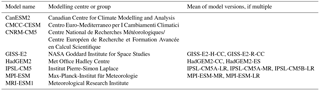
Monthly mean of near-present-day values from 2000 to 2005 of the historical ESM simulations are used for the “CMIP5chl” sensitivity study. The eight models for which such outputs can be obtained through the CMIP5 data portal, and thus used herein, are listed in Table B1.
Table B1List of CMIP5 models containing sea surface chlorophyll concentration data used for the “CMIP5chl” simulation.
The paper was written by WTKH, who designed and performed the experiments, analysed the outputs, and contributed to the implementation of MOA into the model. LI implemented the MOA tracers, ice nucleation due to MOA, as well as the CNT parameterisation for dust following Ickes et al. (2017) into the model and contributed to discussions regarding the technical and scientific details of the study. IT implemented into ECHAM6-HAM2 the SS and MOA emission parameterisations following Long et al. (2011) with an additional sea surface temperature dependence described by Sofiev et al. (2011). MR and DC provided the observed MOA concentrations at Mace Head. UL provided scientific guidance in this study and oversaw the project. The paper has been read, commented, and approved by all co-authors.
The authors declare that they have no conflict of interest.
This article is part of the special issue “BACCHUS – Impact of Biogenic versus Anthropogenic emissions on Clouds and Climate: towards a Holistic UnderStanding (ACP/AMT/GMD inter-journal SI)”. It is not associated with a conference.
The authors would like to acknowledge Jesús Vergara-Temprado for useful
discussions regarding the emission and distribution of MOA in models. Thanks
are also extended to Jurgita Ovadnevaite for discussions regarding AMS
observations of marine organic matter at Mace Head. Lastly, we would like to
thank Susannah Burrows and an anonymous reviewer for the valuable feedback
and suggestions which led to improvement of the manuscript. The research
leading to these results has received funding from the European Union's
Seventh Framework Programme (FP7/2007-2013) project BACCHUS under grant
agreement no. 603445. For the CMIP5 data, we acknowledge the World Climate
Research Programme's Working Group on Coupled Modelling, which is responsible
for CMIP, and the climate modelling groups (listed in
Table B1 of this paper) for producing and making
available their model output. The ECHAM-HAM model is developed by a
consortium composed of ETH Zurich, Max-Planck-Institut für Meteorologie,
Forschungszentrum Jülich, University of Oxford, the Finnish
Meteorological Institute, and the Leibniz Institute for Tropospheric
Research, and managed by the Center for Climate Systems Modeling (C2SM) at
ETH Zurich. Model simulations in this study were performed on the
high-performance computing cluster Euler, maintained by ETH Zurich's
High-Performance Computing (HPC) group under the Scientific IT Services (SIS)
section.
Edited by: Hinrich
Grothe
Reviewed by: Susannah Burrows and one anonymous referee
Abdul-Razzak, H. and Ghan, S. J.: A parameterization of aerosol activation: 2. Multiple aerosol types, J. Geophys. Res.-Atmos., 105, 6837–6844, https://doi.org/10.1029/1999JD901161, 2000. a, b
Bigg, E. K.: Ice Nucleus Concentrations in Remote Areas, J. Atmos. Sci., 30, 1153–1157, https://doi.org/10.1175/1520-0469(1973)030<1153:INCIRA>2.0.CO;2, 1973. a, b
Bonsang, B., Polle, C., and Lambert, G.: Evidence for marine production of isoprene, Geophys. Res. Lett., 19, 1129–1132, https://doi.org/10.1029/92GL00083, 1992. a
Burrows, S. M., Hoose, C., Pöschl, U., and Lawrence, M. G.: Ice nuclei in marine air: biogenic particles or dust?, Atmos. Chem. Phys., 13, 245–267, https://doi.org/10.5194/acp-13-245-2013, 2013. a, b, c
Burrows, S. M., Ogunro, O., Frossard, A. A., Russell, L. M., Rasch, P. J., and Elliott, S. M.: A physically based framework for modeling the organic fractionation of sea spray aerosol from bubble film Langmuir equilibria, Atmos. Chem. Phys., 14, 13601–13629, https://doi.org/10.5194/acp-14-13601-2014, 2014. a
Ceburnis, D., O'Dowd, C. D., Jennings, G. S., Facchini, M. C., Emblico, L., Decesari, S., Fuzzi, S., and Sakalys, J.: Marine aerosol chemistry gradients: Elucidating primary and secondary processes and fluxes, Geophys. Res. Lett., 35, L07804, https://doi.org/10.1029/2008GL033462, 2008. a
Coluzza, I., Creamean, J., Rossi, M. J., Wex, H., Alpert, P. A., Bianco, V., Boose, Y., Dellago, C., Felgitsch, L., Fröhlich-Nowoisky, J., Herrmann, H., Jungblut, S., Kanji, Z. A., Menzl, G., Moffett, B., Moritz, C., Mutzel, A., Pöschl, U., Schauperl, M., Scheel, J., Stopelli, E., Stratmann, F., Grothe, H., and Schmale, D. G.: Perspectives on the Future of Ice Nucleation Research: Research Needs and Unanswered Questions Identified from Two International Workshops, Atmosphere, 8, 138, https://doi.org/10.3390/atmos8080138, 2017. a
Connolly, P. J., Möhler, O., Field, P. R., Saathoff, H., Burgess, R., Choularton, T., and Gallagher, M.: Studies of heterogeneous freezing by three different desert dust samples, Atmos. Chem. Phys., 9, 2805–2824, https://doi.org/10.5194/acp-9-2805-2009, 2009. a, b
DeMott, P. J., Hill, T. C. J., McCluskey, C. S., Prather, K. A., Collins, D. B., Sullivan, R. C., Ruppel, M. J., Mason, R. H., Irish, V. E., Lee, T., Hwang, C. Y., Rhee, T. S., Snider, J. R., McMeeking, G. R., Dhaniyala, S., Lewis, E. R., Wentzell, J. J. B., Abbatt, J., Lee, C., Sultana, C. M., Ault, A. P., Axson, J. L., Diaz Martinez, M., Venero, I., Santos-Figueroa, G., Stokes, M. D., Deane, G. B., Mayol-Bracero, O. L., Grassian, V. H., Bertram, T. H., Bertram, A. K., Moffett, B. F., and Franc, G. D.: Sea spray aerosol as a unique source of ice nucleating particles, P. Natl. Acad. Sci. USA, 113, 5797–5803, https://doi.org/10.1073/pnas.1514034112, 2016. a, b, c, d, e, f, g, h, i, j
Dreischmeier, K., Budke, C., Wiehemeier, L., Kottke, T., and Koop, T.: Boreal pollen contain ice-nucleating as well as ice-binding “antifreeze” polysaccharides, Sci. Rep.-UK, 7, 41890, https://doi.org/10.1038/srep41890, 2017. a
Facchini, M. C., Rinaldi, M., Decesari, S., Carbone, C., Finessi, E., Mircea, M., Fuzzi, S., Ceburnis, D., Flanagan, R., Nilsson, E. D., de Leeuw, G., Martino, M., Woeltjen, J., and O'Dowd, C. D.: Primary submicron marine aerosol dominated by insoluble organic colloids and aggregates, Geophys. Res. Lett., 35, L17814, https://doi.org/10.1029/2008GL034210, 2008. a
Fröhlich-Nowoisky, J., Hill, T. C. J., Pummer, B. G., Yordanova, P., Franc, G. D., and Pöschl, U.: Ice nucleation activity in the widespread soil fungus Mortierella alpina, Biogeosciences, 12, 1057–1071, https://doi.org/10.5194/bg-12-1057-2015, 2015. a
Gantt, B., Meskhidze, N., Facchini, M. C., Rinaldi, M., Ceburnis, D., and O'Dowd, C. D.: Wind speed dependent size-resolved parameterization for the organic mass fraction of sea spray aerosol, Atmos. Chem. Phys., 11, 8777–8790, https://doi.org/10.5194/acp-11-8777-2011, 2011. a, b, c
Gantt, B., Xu, J., Meskhidze, N., Zhang, Y., Nenes, A., Ghan, S. J., Liu, X., Easter, R., and Zaveri, R.: Global distribution and climate forcing of marine organic aerosol – Part 2: Effects on cloud properties and radiative forcing, Atmos. Chem. Phys., 12, 6555–6563, https://doi.org/10.5194/acp-12-6555-2012, 2012. a, b, c
Guelle, W., Schulz, M., Balkanski, Y., and Dentener, F.: Influence of the source formulation on modeling the atmospheric global distribution of sea salt aerosol, J. Geophys. Res.-Atmos., 106, 27509–27524, https://doi.org/10.1029/2001JD900249, 2001. a, b, c
Hoose, C. and Möhler, O.: Heterogeneous ice nucleation on atmospheric aerosols: a review of results from laboratory experiments, Atmos. Chem. Phys., 12, 9817–9854, https://doi.org/10.5194/acp-12-9817-2012, 2012. a
Hoose, C., Lohmann, U., Erdin, R., and Tegen, I.: The global influence of dust mineralogical composition on heterogeneous ice nucleation in mixed-phase clouds, Environ. Res. Lett., 3, 025003, https://doi.org/10.1088/1748-9326/3/2/025003, 2008. a
Hoose, C., Kristjánsson, J. E., and Burrows, S. M.: How important is biological ice nucleation in clouds on a global scale?, Environ. Res. Lett., 5, 024009, https://doi.org/10.1088/1748-9326/5/2/024009, 2010. a
Hu, C., Lee, Z., and Franz, B.: Chlorophyll a algorithms for oligotrophic oceans: A novel approach based on three-band reflectance difference, J. Geophys. Res.-Oceans, 117, C01011, https://doi.org/10.1029/2011JC007395, 2012. a
Huang, W. T. K.: Model data associated with Huang et al. (2018) on ACP, available at: https://data.iac.ethz.ch/MOAacp/, last access: 8 August 2018. a
Ickes, L., Welti, A., and Lohmann, U.: Classical nucleation theory of immersion freezing: sensitivity of contact angle schemes to thermodynamic and kinetic parameters, Atmos. Chem. Phys., 17, 1713–1739, https://doi.org/10.5194/acp-17-1713-2017, 2017. a, b, c, d, e, f, g, h, i, j, k, l, m, n, o, p, q, r, s
Ickes, L., Neubauer, D., and Lohmann, U.: What is triggering ice in mixed-phase clouds in ECHAM-HAM: the importance of ice nucleation, J. Geophys. Res., in preparation, 2018. a
Kanji, Z. A., Ladino, L. A., Wex, H., Boose, Y., Burkert-Kohn, M., Cziczo, D. J., and Krämer, M.: Overview of Ice Nucleating Particles, Meteor. Mon., 58, 1.1–1.33, https://doi.org/10.1175/AMSMONOGRAPHS-D-16-0006.1, 2017. a, b
Knopf, D. A., Alpert, P. A., Wang, B., and Aller, J. Y.: Stimulation of ice nucleation by marine diatoms, Nat. Geosci., 4, 88–90, https://doi.org/10.1038/ngeo1037, 2011. a
Korolev, A.: Limitations of the Wegener–Bergeron–Findeisen Mechanism in the Evolution of Mixed-Phase Clouds, J. Atmos. Sci., 64, 3372–3375, https://doi.org/10.1175/JAS4035.1, 2007. a
Langmann, B., Scannell, C., and O'Dowd, C.: New Directions: Organic matter contribution to marine aerosols and cloud condensation nuclei, Atmos. Environ., 42, 7821–7822, https://doi.org/10.1016/j.atmosenv.2008.09.002, 2008. a
Lapina, K., Heald, C. L., Spracklen, D. V., Arnold, S. R., Allan, J. D., Coe, H., McFiggans, G., Zorn, S. R., Drewnick, F., Bates, T. S., Hawkins, L. N., Russell, L. M., Smirnov, A., O'Dowd, C. D., and Hind, A. J.: Investigating organic aerosol loading in the remote marine environment, Atmos. Chem. Phys., 11, 8847–8860, https://doi.org/10.5194/acp-11-8847-2011, 2011. a, b
Leck, C. and Bigg, E. K.: Source and evolution of the marine aerosol – A new perspective, Geophys. Res. Lett., 32, L19803, https://doi.org/10.1029/2005GL023651, 2005. a
Le Quéré, C., Buitenhuis, E. T., Moriarty, R., Alvain, S., Aumont, O., Bopp, L., Chollet, S., Enright, C., Franklin, D. J., Geider, R. J., Harrison, S. P., Hirst, A. G., Larsen, S., Legendre, L., Platt, T., Prentice, I. C., Rivkin, R. B., Sailley, S., Sathyendranath, S., Stephens, N., Vogt, M., and Vallina, S. M.: Role of zooplankton dynamics for Southern Ocean phytoplankton biomass and global biogeochemical cycles, Biogeosciences, 13, 4111–4133, https://doi.org/10.5194/bg-13-4111-2016, 2016. a
Levkov, L., Rockel, B., Kapitza, H., and Raschke, E.: 3D mesoscale numerical studies of cirrus and stratus clouds by their time and space evolution, Beitr. Phys. Atmos., 65, 35–58, 1992. a
Lohmann, U.: A glaciation indirect aerosol effect caused by soot aerosols, Geophys. Res. Lett., 29, 1052, https://doi.org/10.1029/2001GL014357, 2002. a
Lohmann, U. and Diehl, K.: Sensitivity Studies of the Importance of Dust Ice Nuclei for the Indirect Aerosol Effect on Stratiform Mixed-Phase Clouds, J. Atmos. Sci., 63, 968–982, https://doi.org/10.1175/JAS3662.1, 2006. a
Lohmann, U., Stier, P., Hoose, C., Ferrachat, S., Kloster, S., Roeckner, E., and Zhang, J.: Cloud microphysics and aerosol indirect effects in the global climate model ECHAM5-HAM, Atmos. Chem. Phys., 7, 3425–3446, https://doi.org/10.5194/acp-7-3425-2007, 2007. a, b
Long, M. S., Keene, W. C., Kieber, D. J., Erickson, D. J., and Maring, H.: A sea-state based source function for size- and composition-resolved marine aerosol production, Atmos. Chem. Phys., 11, 1203–1216, https://doi.org/10.5194/acp-11-1203-2011, 2011. a, b, c, d, e, f, g, h, i, j, k, l, m, n, o, p, q
Mann, K. H. and Lazier, J. R. N.: Vertical Structure in Coastal Waters: Coastal Upwelling Regions, Blackwell Publishing Ltd., 163–215, https://doi.org/10.1002/9781118687901.ch5, 2005. a
McCluskey, C. S., Hill, T. C. J., Malfatti, F., Sultana, C. M., Lee, C., Santander, M. V., Beall, C. M., Moore, K. A., Cornwell, G. C., Collins, D. B., Prather, K. A., Jayarathne, T., Stone, E. A., Azam, F., Kreidenweis, S. M., and DeMott, P. J.: A Dynamic Link between Ice Nucleating Particles Released in Nascent Sea Spray Aerosol and Oceanic Biological Activity during Two Mesocosm Experiments, J. Atmos. Sci., 74, 151–166, https://doi.org/10.1175/JAS-D-16-0087.1, 2017. a, b, c
Meskhidze, N., Xu, J., Gantt, B., Zhang, Y., Nenes, A., Ghan, S. J., Liu, X., Easter, R., and Zaveri, R.: Global distribution and climate forcing of marine organic aerosol: 1. Model improvements and evaluation, Atmos. Chem. Phys., 11, 11689–11705, https://doi.org/10.5194/acp-11-11689-2011, 2011. a, b, c
Niemand, M., Möhler, O., Vogel, B., Vogel, H., Hoose, C., Connolly, P., Klein, H., Bingemer, H., DeMott, P., Skrotzki, J., and Leisner, T.: A Particle-Surface-Area-Based Parameterization of Immersion Freezing on Desert Dust Particles, J. Atmos. Sci., 69, 3077–3092, https://doi.org/10.1175/JAS-D-11-0249.1, 2012. a, b, c, d, e, f, g, h, i, j, k, l, m, n, o, p, q, r, s, t, u
O'Dowd, C., Ceburnis, D., Ovadnevaite, J., Bialek, J., Stengel, D. B., Zacharias, M., Nitschke, U., Connan, S., Rinaldi, M., Fuzzi, S., and et al.: Connecting marine productivity to sea-spray via nanoscale biological processes: Phytoplankton Dance or Death Disco?, Sci. Rep.-UK, 5, 14883, https://doi.org/10.1038/srep14883, 2015. a
Rinaldi, M., Fuzzi, S., Decesari, S., Marullo, S., Santoleri, R., Provenzale, A., von Hardenberg, J., Ceburnis, D., Vaishya, A., O'Dowd, C. D., and Facchini, M. C.: Is chlorophyll-a the best surrogate for organic matter enrichment in submicron primary marine aerosol?, J. Geophys. Res.-Atmos., 118, 4964–4973, https://doi.org/10.1002/jgrd.50417, 2013. a, b, c, d, e, f, g, h, i, j, k, l, m, n, o, p, q, r, s, t, u, v, w, x, y
Roelofs, G. J.: A GCM study of organic matter in marine aerosol and its potential contribution to cloud drop activation, Atmos. Chem. Phys., 8, 709–719, https://doi.org/10.5194/acp-8-709-2008, 2008. a
Rogers, R. R. and Yau, M. K.: A short course in cloud physics, Butterworth-Heinemann, 3rd edn., Oxford, UK, 1989. a
Schnell, R. C. and Vali, G.: Biogenic Ice Nuclei: Part I. Terrestrial and Marine Sources, J. Atmos. Sci., 33, 1554–1564, https://doi.org/10.1175/1520-0469(1976)033<1554:BINPIT>2.0.CO;2, 1976. a
Sciare, J., Favez, O., Sarda-Estève, R., Oikonomou, K., Cachier, H., and Kazan, V.: Long-term observations of carbonaceous aerosols in the Austral Ocean atmosphere: Evidence of a biogenic marine organic source, J. Geophys. Res.-Atmos., 114, D15302, https://doi.org/10.1029/2009JD011998, 2009. a, b
Sofiev, M., Soares, J., Prank, M., de Leeuw, G., and Kukkonen, J.: A regional-to-global model of emission and transport of sea salt particles in the atmosphere, J. Geophys. Res.-Atmos., 116, D21302, https://doi.org/10.1029/2010JD014713, 2011. a, b, c, d, e, f, g
Spracklen, D. V., Arnold, S. R., Sciare, J., Carslaw, K. S., and Pio, C.: Globally significant oceanic source of organic carbon aerosol, Geophys. Res. Lett., 35, L12811, https://doi.org/10.1029/2008GL033359, 2008. a
Stevens, B., Giorgetta, M., Esch, M., Mauritsen, T., Crueger, T., Rast, S., Salzmann, M., Schmidt, H., Bader, J., Block, K., Brokopf, R., Fast, I., Kinne, S., Kornblueh, L., Lohmann, U., Pincus, R., Reichler, T., and Roeckner, E.: Atmospheric component of the MPI-M Earth System Model: ECHAM6, J. Adv. Model. Earth Sy., 5, 146–172, https://doi.org/10.1002/jame.20015, 2013. a
Takahashi, K. and Battisti, D. S.: Processes Controlling the Mean Tropical Pacific Precipitation Pattern. Part II: The SPCZ and the Southeast Pacific Dry Zone, J. Climate, 20, 5696–5706, https://doi.org/10.1175/2007JCLI1656.1, 2007. a
Taylor, K. E., Stouffer, R. J., and Meehl, G. A.: An Overview of CMIP5 and the Experiment Design, B. Am. Meteorol. Soc., 93, 485–498, https://doi.org/10.1175/BAMS-D-11-00094.1, 2012. a
Turpin, B. and Lim, H.: Species contributions to PM2.5 mass concentrations: Revisiting common assumptions for estimating organic mass, Aerosol Sci. Technol., 35, 602–610, https://doi.org/10.1080/02786820119445, 2001. a
Vali, G., Christensen, M., Fresh, R. W., Galyan, E. L., Maki, L. R., and Schnell, R. C.: Biogenic Ice Nuclei, Part II: Bacterial Sources, J. Atmos. Sci., 33, 1565–1570, https://doi.org/10.1175/1520-0469(1976)033<1565:BINPIB>2.0.CO;2, 1976. a
Vergara-Temprado, J., Murray, B. J., Wilson, T. W., O'Sullivan, D., Browse, J., Pringle, K. J., Ardon-Dryer, K., Bertram, A. K., Burrows, S. M., Ceburnis, D., DeMott, P. J., Mason, R. H., O'Dowd, C. D., Rinaldi, M., and Carslaw, K. S.: Contribution of feldspar and marine organic aerosols to global ice nucleating particle concentrations, Atmos. Chem. Phys., 17, 3637–3658, https://doi.org/10.5194/acp-17-3637-2017, 2017. a, b, c, d, e, f, g, h, i, j, k, l
Vignati, E., Facchini, M., Rinaldi, M., Scannell, C., Ceburnis, D., Sciare, J., Kanakidou, M., Myriokefalitakis, S., Dentener, F., and O'Dowd, C.: Global scale emission and distribution of sea-spray aerosol: Sea-salt and organic enrichment, Atmos. Environ., 44, 670–677, https://doi.org/10.1016/j.atmosenv.2009.11.013, 2010. a, b, c
Wang, X., Sultana, C. M., Trueblood, J., Hill, T. C. J., Malfatti, F., Lee, C., Laskina, O., Moore, K. A., Beall, C. M., McCluskey, C. S., Cornwell, G. C., Zhou, Y., Cox, J. L., Pendergraft, M. A., Santander, M. V., Bertram, T. H., Cappa, C. D., Azam, F., DeMott, P. J., Grassian, V. H., and Prather, K. A.: Microbial Control of Sea Spray Aerosol Composition: A Tale of Two Blooms, ACS Central Science, 1, 124–131, https://doi.org/10.1021/acscentsci.5b00148, 2015. a
Wiggert, J., Jones, B., Dickey, T., Brink, K., Weller, R., Marra, J., and Codispoti, L.: The Northeast Monsoon's impact on mixing, phytoplankton biomass and nutrient cycling in the Arabian Sea, Deep-Sea Res. Pt. II, 47, 1353–1385, https://doi.org/10.1016/S0967-0645(99)00147-2, 2000. a
Wilks, D. S.: The Stippling Shows Statistically Significant Grid Points: How Research Results are Routinely Overstated and Overinterpreted, and What to Do about It, B. Am. Meteorol. Soc. USA, 97, 2263–2273, https://doi.org/10.1175/BAMS-D-15-00267.1, 2016. a, b
Wilson, T. W., Ladino, L. A., Alpert, P. A., Breckels, M. N., Brooks, I. M., Browse, J., Burrows, S. M., Carslaw, K. S., Huffman, J. A., Judd, C., Kilthau, W. P., Mason, R. H., McFiggans, G., Miller, L. A., Nájera, J. J., Polishchuk, E., Rae, S., Schiller, C. L., Si, M., Temprado, J. V., Whale, T. F., Wong, J. P. S., Wurl, O., Yakobi-Hancock, J. D., Abbatt, J. P. D., Aller, J. Y., Bertram, A. K., Knopf, D. A., and Murray, B. J.: A marine biogenic source of atmospheric ice-nucleating particles, Nature, 525, 234–238, https://doi.org/10.1038/nature14986, 2015. a, b, c, d, e, f, g, h, i, j, k, l, m, n
Yun, Y. and Penner, J. E.: An evaluation of the potential radiative forcing and climatic impact of marine organic aerosols as heterogeneous ice nuclei, Geophys. Res. Lett., 40, 4121–4126, https://doi.org/10.1002/grl.50794, 2013. a, b, c
Zhang, K., O'Donnell, D., Kazil, J., Stier, P., Kinne, S., Lohmann, U., Ferrachat, S., Croft, B., Quaas, J., Wan, H., Rast, S., and Feichter, J.: The global aerosol-climate model ECHAM-HAM, version 2: sensitivity to improvements in process representations, Atmos. Chem. Phys., 12, 8911–8949, https://doi.org/10.5194/acp-12-8911-2012, 2012. a