the Creative Commons Attribution 4.0 License.
the Creative Commons Attribution 4.0 License.
 | 06 Aug 2018
Forecasting carbon monoxide on a global scale for the ATom-1 aircraft mission: insights from airborne and satellite observations and modeling
Junhua Liu
Leslie Lait
Róisín Commane
Bruce Daube
Steven Wofsy
Austin Conaty
Paul Newman
Michael Prather
The first phase of the Atmospheric Tomography Mission (ATom-1) took place in July–August 2016 and included flights above the remote Pacific and Atlantic oceans. Sampling of atmospheric constituents during these flights is designed to provide new insights into the chemical reactivity and processes of the remote atmosphere and how these processes are affected by anthropogenic emissions. Model simulations provide a valuable tool for interpreting these measurements and understanding the origin of the observed trace gases and aerosols, so it is important to quantify model performance. Goddard Earth Observing System Model version 5 (GEOS-5) forecasts and analyses show considerable skill in predicting and simulating the CO distribution and the timing of CO enhancements observed during the ATom-1 aircraft mission. We use GEOS-5's tagged tracers for CO to assess the contribution of different emission sources to the regions sampled by ATom-1 to elucidate the dominant anthropogenic influences on different parts of the remote atmosphere. We find a dominant contribution from non-biomass-burning sources along the ATom transects except over the tropical Atlantic, where African biomass burning makes a large contribution to the CO concentration. One of the goals of ATom is to provide a chemical climatology over the oceans, so it is important to consider whether August 2016 was representative of typical boreal summer conditions. Using satellite observations of 700 hPa and column CO from the Measurement of Pollution in the Troposphere (MOPITT) instrument, 215 hPa CO from the Microwave Limb Sounder (MLS), and aerosol optical thickness from the Moderate Resolution Imaging Spectroradiometer (MODIS), we find that CO concentrations and aerosol optical thickness in August 2016 were within the observed range of the satellite observations but below the decadal median for many of the regions sampled. This suggests that the ATom-1 measurements may represent relatively clean but not exceptional conditions for lower-tropospheric CO.
- Article
(3267 KB) -
Supplement
(4065 KB) - BibTeX
- EndNote


The first phase of the NASA Atmospheric Tomography Mission (ATom-1) (https://espo.nasa.gov/atom, last access: 30 July 2018) took place in July–August 2016. The aircraft completed a circuit beginning in Palmdale, California, and traversing the remote Pacific and Atlantic oceans, providing an unprecedented picture of the chemical environment at a wide range of latitudes over the remote oceans. Major goals of the ATom mission include identifying chemical processes that control the concentrations of short-lived climate forcers, quantifying how anthropogenic emissions affect chemical reactivity globally, and identifying ways to improve the modeling of these processes.
Chemical forecasts from the Goddard Earth Observing System Model version 5 (GEOS-5) model provided insight into the chemical environments and sources of pollution for the diverse regions sampled during the ATom-1 campaign. GEOS-5 forecasts help determine the source regions and emission types that contribute to the trace gas and aerosol concentrations measured during ATom, which is directly relevant to the goal of quantifying how anthropogenic emissions affect global chemical reactivity. GEOS-5 supports numerous aircraft missions, and validation of the model forecasts is important for developing confidence in and understanding the limitations of chemistry forecasting for aircraft missions. The ATom dataset, which uses unbiased sampling rather than chasing plumes, provides a unique opportunity to validate the overall performance of the GEOS-5 model on a global scale.
One of the goals of ATom is to provide an observation-based climatology of important atmospheric constituents and their reactivity in the remote atmosphere. Consequently, it is important to examine whether the ATom observations are temporally and spatially representative of the broader remote atmosphere. Prather et al. (2017) examined the ability of observations from a single path to represent the variability of a broader geographic region but noted that year-to-year and El Niño–Southern Oscillation (ENSO) variability could also be important. Year-to-year variability in meteorology and emissions both contribute to interannual variability in trace gases and aerosols, so it is important to consider the temporal representativeness of a single season sampled by ATom. For example, ENSO is a major driver of variability in ozone distributions (Ziemke and Chandra, 2003), and large biomass burning (BB) events during El Niño years increase concentrations of trace gases including CO and CO2 (Langenfelds et al., 2002). Biomass burning plays a particularly strong role in driving the interannual variability of CO (e.g., Novelli et al., 2003; Kasischke et al., 2005; Duncan and Logan, 2008; Strode and Pawson, 2013; Voulgarakis et al., 2015). The impacts of large biomass burning events during El Niño events are visible in satellite observations of CO (e.g., Edwards et al., 2004, 2006; Logan et al., 2008; Liu et al., 2013). Pfister et al. (2010) used a chemistry transport model (CTM) as well as satellite data to examine the CO sources and transport over the Pacific during the INTEX-B mission compared to previous years. They found biomass burning to be the largest contributor to interannual variability, despite its lower emissions compared to fossil fuel sources. Here we show how the time and place of ATom-1 measurements fit into a global, multi-year climatology of CO. In particular, we assess the extent to which measurements from the ATom-1 period represent the CO and aerosol distributions over the last decade and a half.
In this study, we place the August 2016 ATom observations in the context of interannual variability and assess the contributions of different emission sources to the various regions sampled during the campaign. We focus on CO, a tracer of incomplete combustion whose lifetime of 1–2 months allows long-range transport to the remote oceans. Section 2 describes the model and observations used in this analysis. Section 3 compares the GEOS-5 CO to observations. Section 4 discusses the global distribution of CO and presents the relative CO source contributions to the regions sampled by ATom. Section 5 presents an analysis of the interannual variability in CO and aerosol optical thickness seen in satellite observations to assess how well August 2016 observations represent climatological August conditions. Section 6 summarizes our conclusions.
2.1 ATom observations
ATom-1 flew transects through the Pacific, Southern, Atlantic and Arctic oceans with the NASA DC-8 aircraft in August 2016. Each of the 11 flights included sampling from the boundary layer to the top of the aircraft range (39 kft). We use the ATom-1 data (July–August 2016) (Atom Science Team, 2017; Wofsy et al., 2018) for comparison with the model forecasts and analyses.
We take ATom-1 CO observations from the Harvard quantum cascade laser spectrometer (QCLS) instrument (Santoni et al., 2014), which has a history of successful measurements during the HIAPER Pole-to-Pole Observations (HIPPO) campaign. Briefly, the instrument uses a pulsed quantum cascade laser at 2160 cm−1 to measure absorption of CO through an astigmatic multi-pass sample cell (with 76 m path length), with detection using a liquid-nitrogen-cooled HgCdTe detector. A separate laser and detector are used to measure methane and nitrous oxide in the same cell. In-flight calibrations were conducted with gases traceable to the NOAA WMO (X2014) scale, with calibration of tanks before ATom-1 and after ATom-2 (February 2017) showing no significant change in the CO concentration in the gas standards. The inlet for the instrument was specially designed for the DC-8 aircraft. The QCLS observations have an accuracy and precision of 3.5 and 0.15 ppb, respectively. The QCLS observations used in this analysis are being archived at the Oak Ridge National Laboratory Distributed Active Archive Center (ORNL DAAC, https://doi.org/10.3334/ORNLDAAC/1604).
2.2 Satellite observations
We use satellite observations that cover more than a decade to examine the interannual variability of CO and aerosols. We focus on satellite observations because they provide broad coverage over the oceans, where surface data are sparse. The Measurement of Pollution in the Troposphere (MOPITT) instrument, which flies on the Terra satellite, provides CO observations beginning in 2000 (Edwards et al., 2004). We use the version 6 thermal infrared (TIR) level 3 product (Deeter et al., 2014). The MOPITT TIR averaging kernels show high sensitivity to CO between 700 and 500 hPa (Emmons et al., 2007). We use the CO column and 700 hPa CO retrievals.
The Microwave Limb Sounder (MLS) (Waters et al., 2006), which flies on the Aura satellite, provides useful observations of CO down to 215 hPa (Livesey et al., 2008) beginning in 2004. We use the version 4.2 level 2 data for the 215 hPa level with the recommended quality, status, precision, and convergence criteria. Although MLS data overlap with ATom only at the highest flight levels, MLS and MOPITT provide complementary views of CO in the upper troposphere/lower stratosphere (UTLS) and lower troposphere, respectively. The MOPITT averaging kernels include some sensitivity to the 200 hPa level, implying a small overlap between the MOPITT and MLS observations.
The Moderate Resolution Imaging Spectroradiometer (MODIS) instrument on the Aqua satellite provides column aerosol optical thickness (AOT) data beginning in 2002. We use MODIS data in this analysis because they provide a relatively long data record. We use the Collection 6 level 2 (MYD04_L2) (Levy et al., 2015) 550 nm AOT data over oceans aggregated into 0.5∘ grid boxes and then take monthly means with the daily data weighted according to the quality assurance.
2.3 Model description
We use chemical forecasts and analyses from the GEOS-5 forward processing (FP) system to quantify the contribution of different emission sources to the observed CO distribution and to identify the origin of observed plumes. A global model is necessary for this analysis since CO is transported globally. The FP stream from the Global Modeling and Assimilation Office (GMAO) generates GEOS-5 forecast products as well as assimilation products using the most current system approved for near-real-time production. We use the FP system in our study because it is the system used to generate forecasts that are used during ATom and other aircraft missions and is thus relevant to future mission and flight planning. The GEOS-5 model (Molod et al., 2015) is a global general circulation model (GCM) with 72 vertical levels reaching from the surface to 1 Pa. The assimilation system is described in Rienecker et al. (2008, 2011), and includes assimilation of ozone measurements from the Ozone Monitoring Instrument (OMI) and MLS, and aerosol optical depth as well as meteorological variables. The forward processing system produces output on 72 model levels or 42 pressure levels with ∘ horizontal resolution. Our study uses the pressure level output.
The GEOS-5 FP system (Lucchesi, 2017) simulates the transport of CO as well as tagged CO tracers from specific regions and sources, which helps track the transport of pollution outflow. Tagged tracers are available for BB globally as well as biomass burning from Eurasia, North America, Africa, and Central and South America, and for non-BB sources globally and from Europe, Asia, and North America. Non-BB sources include fossil fuels, biofuels, CO from oxidation of biogenic volatile organic compounds (VOCs), and CO from methane oxidation, as described in Ott et al. (2010). Figure S1 in the Supplement shows the regions included in each tagged tracer. Bian et al. (2013) used observations of dichloromethane and acetonitrile from the ARCTAS mission to validate the anthropogenic and biomass burning CO tracers, respectively.
Daily-varying biomass burning emissions come from the Quick Fire Emission Dataset (QFED) version 2 (Darmenov and da Silva, 2015), which is based on fire radiative power from the MODIS instrument. Thus the BB emissions include day-to-day and interannual variability, but the non-BB sources and the OH fields use monthly means and lack daily-scale variability and interannual variability. Table 1 presents the August emission inputs for the major regions considered. CO emissions are then scaled up by 20 % for fossil fuels and 11 % for biomass burning to account for CO production from co-emitted VOCs, since VOCs are not explicitly carried in the GEOS-5 FP chemical mechanism. This approach was developed by Duncan et al. (2007) to account for the CO source from non-methane hydrocarbon oxidation.
CO from methane oxidation is included in the non-BB tagged tracers for the regions in which oxidation occurred. For example, if methane is oxidized over North America, the resulting CO is included in the North American non-BB tracer. The monthly mean methane fields come from a GMI chemistry and transport model (CTM) simulation, which uses prescribed zonal mean surface concentrations. CO is lost by reaction with OH using fixed monthly OH fields archived from the GMI CTM. Figure S2 shows the methane and OH fields included in the FP system.
Table 1Regional August 2016 CO emission totals in the GEOS-5 FP simulations.
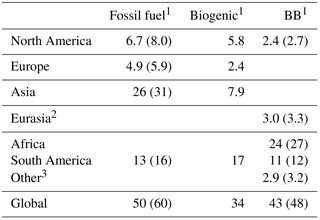
1Emissions are in units of terragram (Tg). Values in parentheses include the 20 and 11 % scaling factors for fossil fuels and biomass burning, respectively, to account for CO production from VOC oxidation. 2The Eurasian tagged tracer for BB CO includes emissions from Europe and northern Asia but excludes southern Asia. 3Other fossil fuel emissions include emissions from Africa and South America, while other BB emissions exclude those regions since they are tagged separately. Other BB does include southern Asia as well as Australia.
During the ATom mission, the GEOS-5 model was engaged to provide chemical forecasts for each flight that include the major chemical species and, for CO, tagged tracers for different sources. The chemical forecasts were used together with meteorological forecasts for day-to-day flight planning, although flight tracks were intentionally not altered to chase specific chemical features to avoid a highly biased sampling of pollution. The chemical forecasts provide the ATom team with a preview of the chemical environments that the flight is expected to sample, including the location of pollution, biomass burning, or dust plumes; regions of substantial but well-mixed anthropogenic pollution; and cleaner regions. The forecasts also provide a broader spatial context for the observations, since the three-dimensional model output shows the spatial extent of features that intersect the flight track.
We examine the performance of the GEOS-5 forecasts by comparing the simulated CO to the QCLS observations. The forecasts provided during the mission used forecast wind fields, with the forecast lead time varying depending on the timing of the flight. For consistency, the results shown here use the CO simulated with the assimilated wind fields, but we note that similar features were seen for the CO simulated with the forecast winds, as further discussed in Sect. 3.1.2. For the model results, we do not apply temporal interpolation between the model output frequency (6 h). Instead, we sample the model forecasts at the time closest to the midpoint of each flight segment. For comparison with observations, the 3-D model forecast was interpolated to the longitude, latitude, and pressure given in the 10 s merges of the ATom measurements.
3.1 Analysis of CO along the meridional flight tracks
Table 2Mean and standard deviations in CO along Atlantic and Pacific flight tracks.
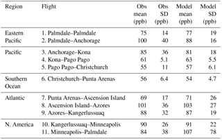
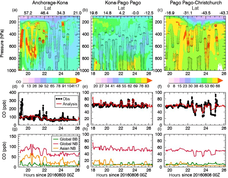
Figure 1Curtain plot of CO (ppb) from the GEOS-5 analysis as a function of time and pressure overplotted with the model tropopause (gray line) and QCLS CO observations (circles) (a, b, c) for the (a) Anchorage–Kona flight, (b) Kona–Pago Pago flight, and (c) Pago Pago–Christchurch flight. Axis ranges vary between panels due to the large range of concentrations encountered. The top x axis indicates the latitudes of the flight track. (d–f) The GEOS-5 CO interpolated to the flight track (red line) is compared to the observations (black circles). (g–h) Tagged tracer contributions to the GEOS-5 CO.
We compare CO from GEOS-5 to the QCLS CO observations for specific flights, using the 10 s merge files. The GEOS-5 CO is taken from the 3-D field at the time closest to the midpoint of the flight and interpolated in space to the flight track. The ATom flight tracks are shown in Fig. S3. Although we briefly discuss the other flights as well, we focus on two sections of the ATom-1 circuit: the north–south flights through the Pacific and the south–north flights through the Atlantic. These two transects allow us to examine the transition from northern hemispheric to tropical to southern hemispheric influence.
3.1.1 Pacific legs
Figure 1 shows CO from the three Pacific flights spanning Anchorage, Alaska, to Christchurch, New Zealand. The top panels show the GEOS-5 curtain of CO along the flight track, with the QCLS observations overplotted in circles. The observations show higher values of CO in the first half of the Anchorage–Kona flight compared to the other portions of the Pacific, and this feature is reproduced in GEOS-5 as well. GEOS-5 agrees well with the observed mean value for CO on this flight (Table 2). Tagged tracers (Fig. 1 bottom panels) show that non-BB sources, especially from Asia, are the dominant contributor to CO levels throughout the Pacific, and the decrease in Asian non-BB CO explains the observed decrease in CO as the flights move south.
The observations show plumes of enhanced CO scattered throughout all three Pacific flights, although they are most intense in the North Pacific, as seen in the Anchorage–Kona flight. GEOS-5 typically reproduces the timing of these plumes, but the magnitude is usually underestimated, particularly for the strongest plumes. This leads to an underestimate of the observed standard deviation of the CO on the Palmdale–Anchorage (Fig. S4) and Anchorage–Kona flights (Table 2). In addition to biases in emissions, observations often show fine-scale structures too small for the model to resolve (Hsu et al., 2004), and underestimating the concentrations in strong plumes is a common problem for global models (e.g., Heald et al., 2003). Either biases in emissions or insufficient vertical or horizontal model resolution may thus be responsible for the underestimate. The tagged tracer for biomass burning shows a small increase at the time of the underestimated plumes near hour 22 of the Anchorage–Kona flight (Fig. 1d, g), suggesting that those underestimates are due to the insufficient magnitude of the simulated biomass burning plumes. An exception is in the tropical Pacific (Kona–Pago Pago flight), in which GEOS-5 predicted some enhancements, driven by fossil fuels, not seen in the observations. Tagged tracers indicate that Asian non-BB CO drove many of the observed enhancements, while others were due to biomass burning.
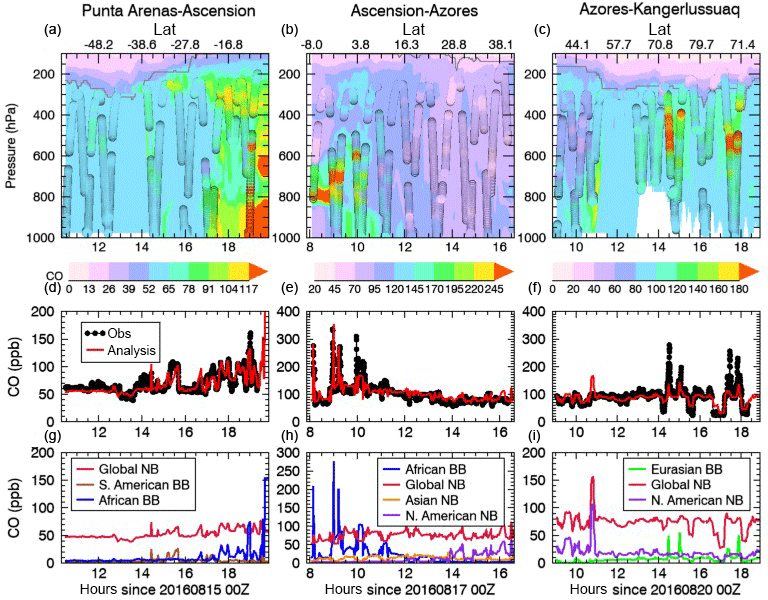
Figure 2As in Fig. 1 but for the Atlantic flights: (a, d, g) Punta Arenas to Ascension Island, (b, e, h) Ascension Island to the Azores, and (c, f, i) Azores to Kangerlussuaq.
In the South Pacific (Pago Pago–Christchurch segment), the flight sampled the stratosphere three times, with CO levels decreasing to approximately 30 ppb, as shown in Fig. 1c. As expected from stratospheric chemistry and seen in previous observations, both ATom-1 and GEOS-5 show a strong decrease in CO as the flight rises above the tropopause, with GEOS-5 underestimating the observed gradient. Both the model and measurements show tropospheric CO less than 90 ppbv along the flight route with slightly elevated CO above 600 hPa around 22:00 and 00:00. For this flight and the subsequent flight to Punta Arenas, all observations are in the Southern Hemisphere and the mean values for both ATom-1 and GEOS-5 agree within the range 54–57 ppb (Table 2, Fig. S5).
3.1.2 Atlantic legs
The ATom flights traversed the Atlantic from south to north, beginning in Punta Arenas, Chile, and ending in Kangerlussuaq, Greenland. Figure 2 shows the Atlantic flights from Punta Arenas to Ascension Island to the Azores to Kangerlussuaq. GEOS-5 has an excellent simulation of background CO values seen on these flights, with the mean values falling within 2 ppb of the observations (Table 2), while the mean observed values for each flight shift from 69 to 101 to 88 ppb. The observations show plumes of high CO intersecting the flight track on all three flights. GEOS-5 also shows plumes of enhanced CO at these locations, but the magnitude is often underestimated (Fig. 2d–f), especially for the Azores–Kangerlussuaq flight. Figure S6 shows the CO results for the Azores–Kangerlussuaq flight using forecast wind fields and illustrates the temporal evolution of CO plumes along the flight track. Comparison of Fig. S6 with Fig. 2f shows that the impact of using analysis versus forecast wind fields is small for this flight since the forecasts already capture the timing of the plumes.
Non-BB sources dominate the background CO levels on all three flights. However, biomass burning plays a dominant role in the plumes of high CO (Fig. 2g–i). South American biomass burning leads to CO enhancements between T14 and T16 of the Punta Arenas–Ascension Island flight. In the later portion of that flight, biomass burning from Africa leads to strong CO plumes. Strong plumes of African biomass burning are also seen at the beginning of the Ascension Island–Azores flight. GEOS-5 shows a strong plume around 800 hPa for the first hour of the flight, which agrees well with observations (Fig. 2b, d). The observations show additional strong plumes in the next hour between 600 and 700 hPa. These plumes are present but underestimated in GEOS-5, possibly due to errors in the magnitude of the emissions or the placement or extent of the plumes. The placement and strength of simulated plumes is sensitive to the injection height of the biomass burning, which is a source of uncertainty. In addition, plumes in models tend to dissipate more quickly than in observations due to the numerical effects of limited model resolution (Eastham and Jacob, 2017).
The non-BB contribution to CO in the Atlantic reflects a mixture of global sources. Asian sources make a notable contribution to the non-BB CO variability in the tropics (first half of the Ascension Island–Azores flight), but as expected N. American sources become more dominant in the second half. In the northern (later) portion of the Azores–Kangerlussuaq flight (Fig. 2), GEOS-5 attributes the observed plumes to Eurasian biomass burning but underestimates their magnitude. This flight also crosses the tropopause, and both ATom-1 and GEOS-5 show a corresponding dip in CO concentrations. GEOS-5 predicts a plume of enhanced CO due to N. American emissions around 11Z of the Azores–Kangerlussuaq flight that is not seen in the observations (Fig. 2f, i). A similar error is made in the Kangerlussuaq–Minneapolis flight (Fig. S5). This could be due either to an error in the assumed N. American sources or to misplacement of the plume by the model. A large overestimate of CO at the end of the Minneapolis–Palmdale flight also points to a potential error in North American emissions from either fossil fuels or biomass burning.
3.2 Model evaluation summary
We summarize the comparison between the CO simulated by the GEOS-5 analyses and the QCLS observations in Fig. 3. The majority of points lie near the one-to-one line, indicating good overall agreement between the GEOS-5 and observed CO distributions. The higher concentrations in the tropical Atlantic compared to the tropical Pacific are evident in both the observations and model. Figure 3 also reveals occasional model overestimates of CO on flights over North America (green triangles), as well as underestimates of high-CO plumes over the North Pacific and tropical Atlantic. An underestimate of Eurasian biomass burning contributes to the model underestimates in the North Pacific and North Atlantic, and has implications for ozone production in aged BB plumes. Globally, the correlation of simulated and observed CO with 5 min binning is r=0.69. Correlations for the Pacific, Atlantic, and North America are 0.72, 0.80, and 0.80, respectively, while the correlation for the Southern Ocean is 0.053. The poor correlation for the Southern Ocean reflects the very low variability of CO in this region. The model performs far better at capturing the larger gradients present in the other regions. In general, the good agreement between model outputs and observations attests to the model forecasting skill and suggest the suitability of using GEOS-5 forecast products to guide the design and execution of aircraft campaigns.
4.1 Global CO distribution
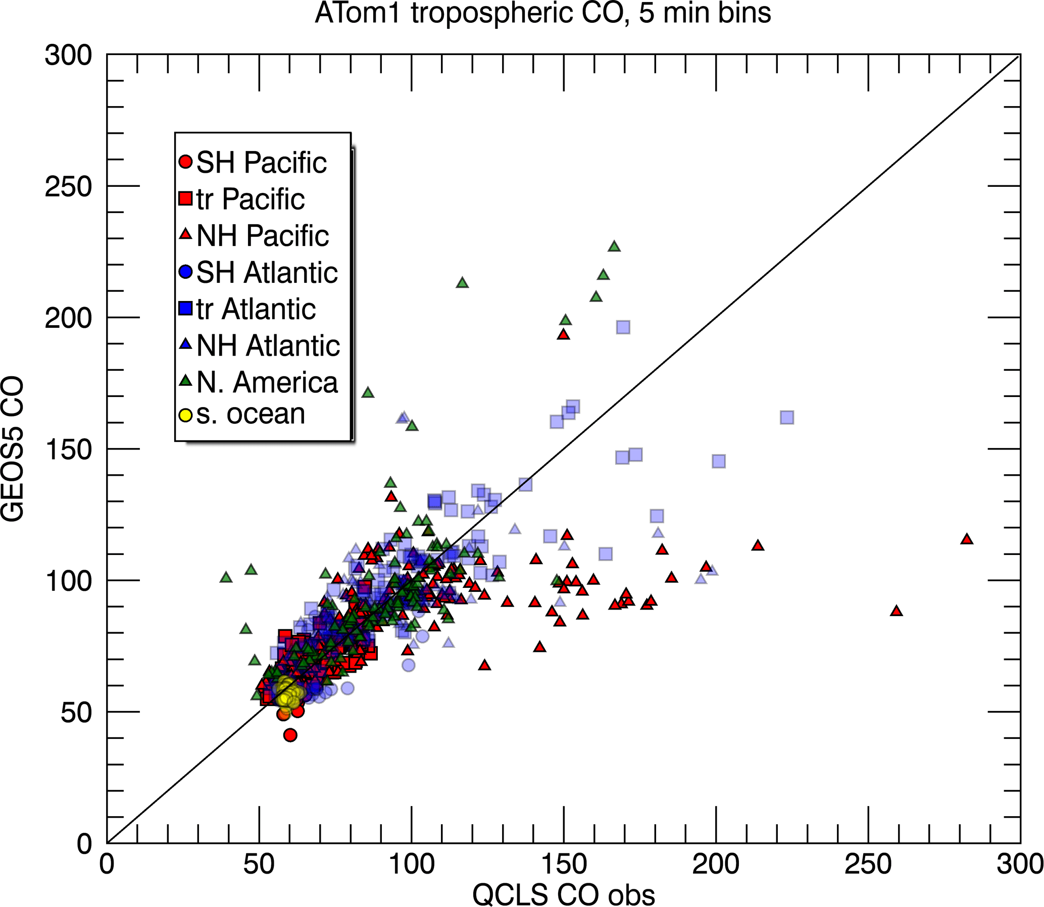
Figure 3GEOS-5 simulated CO vs. QCLS CO observations for all ATom-1 flights averaged into 5 min bins. CO is in units of ppb. Pacific flights are shown in red, Atlantic flights in blue, N. American flights in green, and Southern Ocean flights in yellow. Circles indicate Southern Hemisphere points, triangles indicate Northern Hemisphere points, and squares indicate tropical points. The one-to-one line is overplotted in black.
Figure 4 compares CO from GEOS-5 to the QCLS CO observations for the ATom-1 circuit including the 11 total flight segments. The GEOS-5 CO is taken from the analysis closest to the midpoint of the flight time and interpolated to the flight track following the longitude, latitude, and pressure given in the observations. We average both model CO and ATom measurements into one point per 360 s for easier visualization.
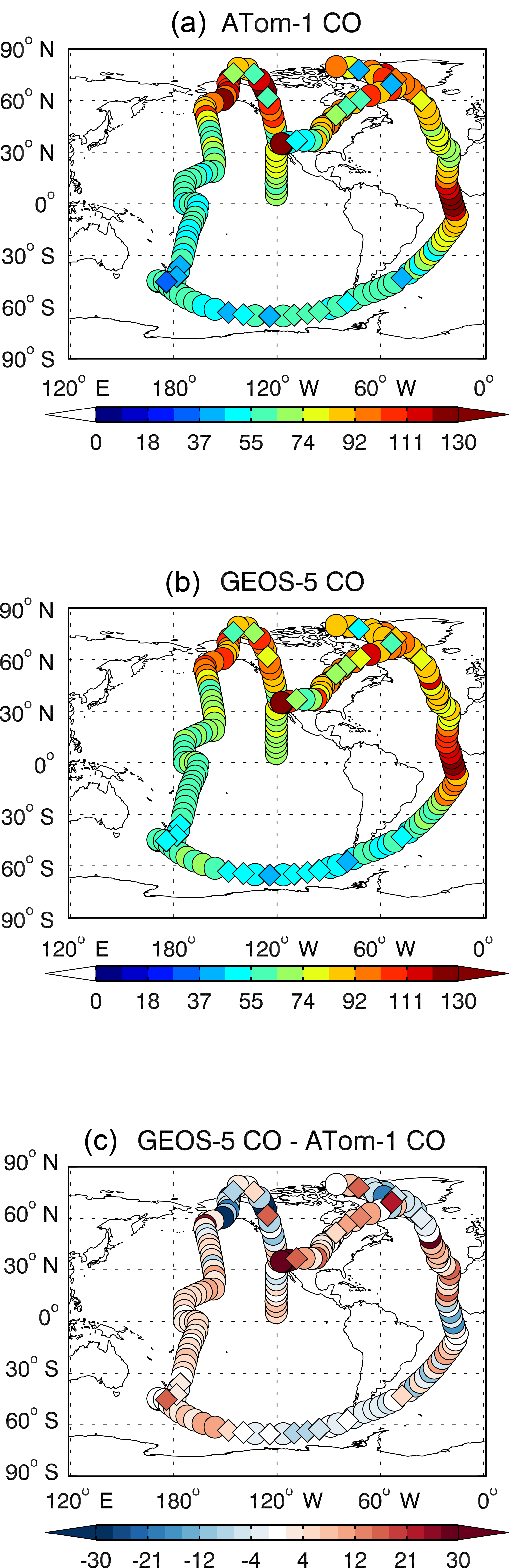
Figure 4CO (ppb) from the (a) QCLS observations, (b) GEOS-5 analysis, and (c) the GEOS-5–observation difference for the ATom-1 circuit including all 11 research flight segments. The GEOS-5 CO is taken from the analysis closest to the midpoint of the flight time and interpolated to the flight track following the longitude, latitude, and pressure given in the observations. Both model forecast and ATom measurements are averaged into a sample rate of one per 360 s. Data in the troposphere are plotted in a circle, while data in the stratosphere are plotted in a diamond, based on the GEOS-5 tropopause.
Both model simulations and measurements show polluted air with higher CO mixing ratios in the Northern Hemisphere than that in the Southern Hemisphere in August 2016. Over the northern hemispheric polar region, the observations indicate highly polluted air with CO maxima occurring over Alaska and northwest Canada, features also seen in the GEOS-5 simulation. Over the Atlantic section, CO maxima with slightly lower values occur around the same latitude over west Greenland as shown both in observations and model simulation. CO over the northernmost locations along the ATom-1 circuit see some low values both in model and observations, particularly north of 30∘ N and south of 40∘ S, due to the measurements occurring in the stratosphere or occurring in the upper troposphere with stratospheric influence. Both model and observations indicate that the air is relatively clean over the Pacific south of 30∘ N with CO less than 70 ppb and the CO minimum around 60∘ S over the eastern South Pacific. Over the Atlantic section, both model and observations show low CO concentration south of 30∘ S but show a strong CO maximum over the tropical Atlantic (5S–5N) with CO greater than 120 ppb. This high CO is mainly driven by Southern Hemisphere BB. CO is slightly lower between 30 and 60∘ N compared to that over the tropical Atlantic and Greenland. The similarity between GEOS-5 and ATom-1 variability in neighboring points is due in part to the vertical profiling, which places horizontally extensive biomass burning layers in the model and presumably also the atmosphere at the same point along the track.
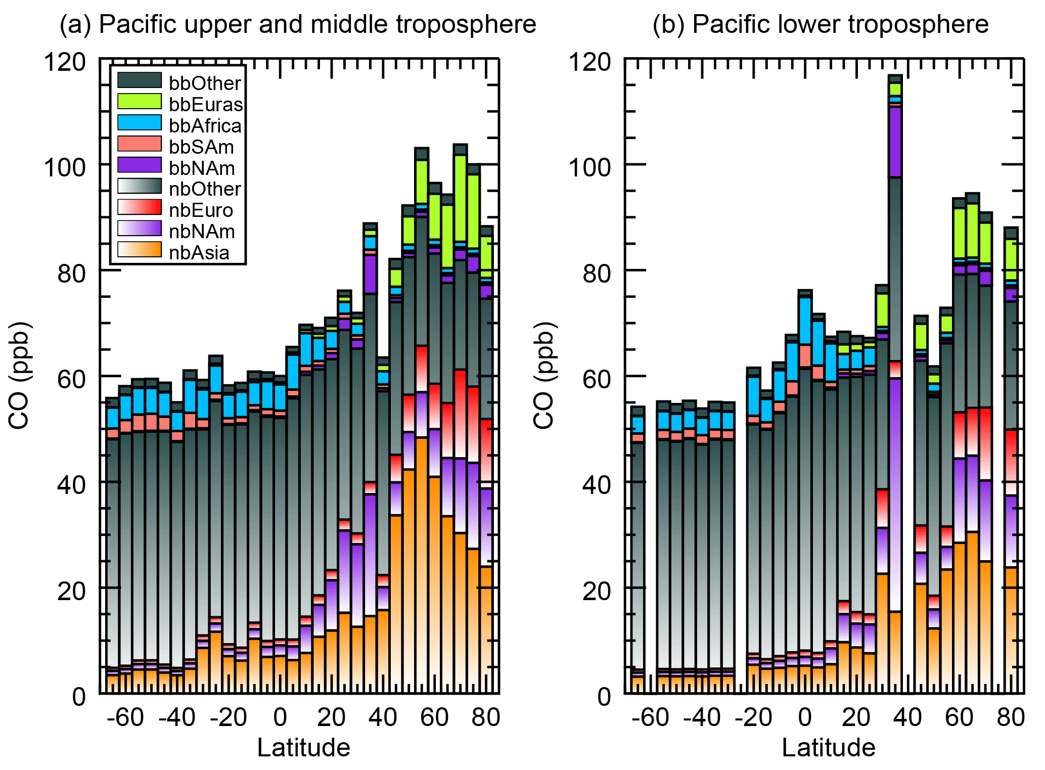
Figure 5The contribution of each tagged CO tracer over the Pacific in the (a) upper and middle troposphere (pressure < = 850 hPa) and (b) lower troposphere (pressure > 850 hPa). Data from multiple flights over the region between 120∘ E and 110∘ W are included, with each bar representing data averaged over a 5∘ latitude bin. Shaded bars represent non-BB CO from Asia (orange), N. America (purple), Europe (red), and the rest of the world (gray). Solid bars represent BB CO from N. America (purple), S. America (pink), Africa (cyan), Eurasia (green), and the rest of the world (gray).
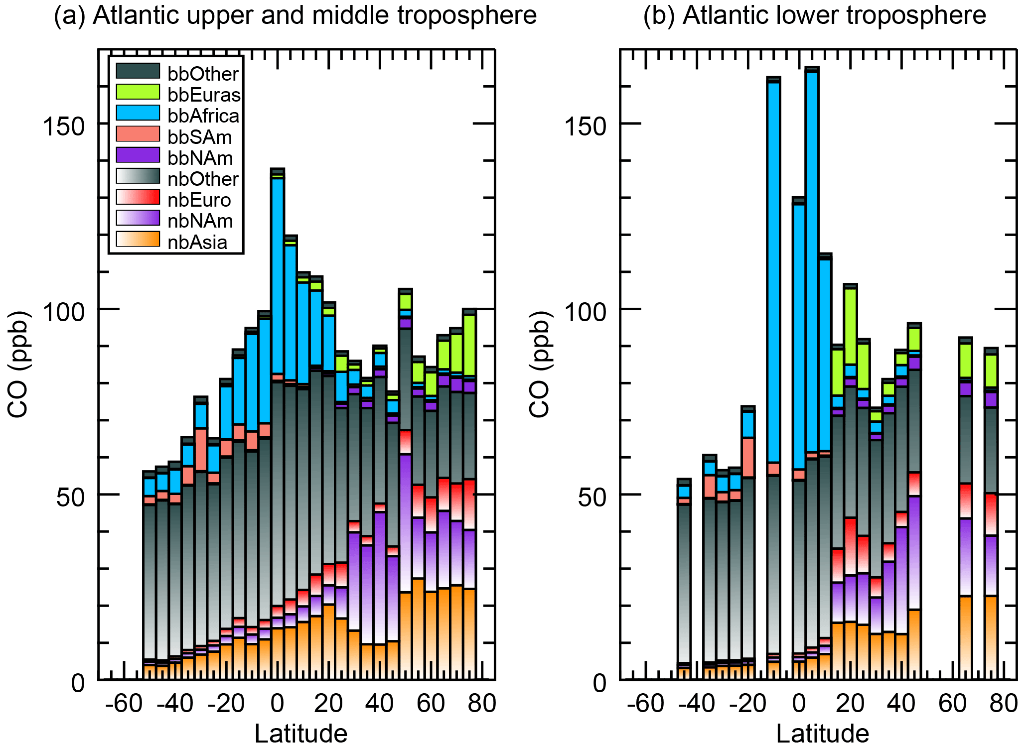
Figure 6As in Fig. 5 but for the Atlantic. Data from multiple flights over the region 0–60∘ W are included, with each bar representing data averaged over a 5∘ latitude bin.
4.2 CO source contributions
We calculate the contribution of different CO sources to the total simulated CO using the GEOS-5 tagged CO tracers sampled along the ATom flight tracks. This analysis provides a picture of the dominant sources affecting the constituent concentrations observed during ATom-1 for different regions of the atmosphere. The tagging of CO sources includes both BB and non-BB from four continental areas, with all other sources put into the “other” bin. Other BB sources are small, but other non-BB sources are quite large as they include all natural sources as well as atmospheric photochemical sources such as methane oxidation.
Figure 5 shows the contribution of each tagged tracer over the Pacific Ocean from 120∘ E to 110∘ W, averaged over 5∘ latitude bins. Non-biomass-burning sources dominate at all latitudes, due in part to the inclusion of CO from methane oxidation in addition to fossil fuel sources in these tracers. The oxidation of methane over the remote oceans contributes to the large magnitude of “other non-BB” sources over the southern latitudes of the Pacific. Asian non-BB sources make the largest contribution to middle- and upper-tropospheric CO (Fig. 5a) at the midlatitudes of the North Pacific, with smaller contributions from N. American and European non-BB sources. The largest biomass burning contribution comes from Africa in the Southern Hemisphere and tropics, switching to Eurasia in the northern latitudes.
Figure 5b shows the relative contributions in the lower troposphere, including the marine boundary layer and defined here as pressures greater than 850 hPa. Missing bars indicate latitudes where no ATom-1 measurements were made in the lower troposphere. Asian non-BB CO makes a smaller contribution in the lower troposphere than in the middle and upper troposphere. A strong CO maximum around 30∘ N is more pronounced in the lower troposphere than above. This bin is not representative of the remote Pacific as it includes Palmdale, California, with large contributions from local North American BB and non-BB sources.

Figure 7Percent contributions of tagged tracers to total CO for each flight. Exploded slices represent the biomass burning (bb) tracers: North American (purple), S. American (salmon), African (cyan), Eurasian (green), and other (dark gray). The non-biomass-burning (nb) tracers are for Asia (orange), N. America (lavender), Europe (red), and other (light gray).
The Atlantic flights (0–60∘ W) show a large contribution from other non-BB sources in the Southern Hemisphere with increasing contributions from Asian, N. American, and European non-BB CO as the flight moves northward (Fig. 6), similar to the picture over the Pacific. However, the Atlantic receives a larger contribution from biomass burning, particularly from Africa, over the tropics. The contribution from African BB is strong throughout the troposphere but is particularly pronounced in the lower troposphere, where it exceeds 100 ppb in the bins centered at 10∘ S and 5∘ N.
We also examine the tagged tracer contributions for each flight, including all altitudes sampled by the flight (Fig. 7, Table S1). Flights occurring in the tropics and Southern Hemisphere (flights 1, 4–8) receive 44–75 % of the total CO from other non-BB sources. Other non-biomass-burning sources include all non-biomass-burning sources located outside North America, Europe, and Asia. The contribution from methane oxidation in addition to Southern Hemisphere emissions explains this large contribution. Flight 8 has a somewhat lower percent contribution from other non-BB sources than the other Southern Hemisphere and tropical flights due to the higher percent contribution from African biomass burning. In contrast, the Northern Hemisphere flights have a larger contribution from Northern Hemisphere source regions. Asian non-BB explains over a third of the total CO for the North Pacific flights (flights 2–3), while Asian and N. American non-BB sources make comparable contributions to the North Atlantic and N. American flights (flights 9–11).
Since Figs. 5 and 6 reveal differences in source contributions between the lower troposphere and the middle and upper troposphere, we also examine the source contributions to each flight for the lower troposphere (pressure >850 hPa) only (Fig. S7). Asian sources make a larger percent contribution to the Pacific flights (flights 0–4) when all flight altitudes are considered rather than the lower troposphere alone. Regional sources such as African biomass burning for flights 6 and 7 and N. American sources for flights 9 and 10 make a larger percent contribution in the lower troposphere.
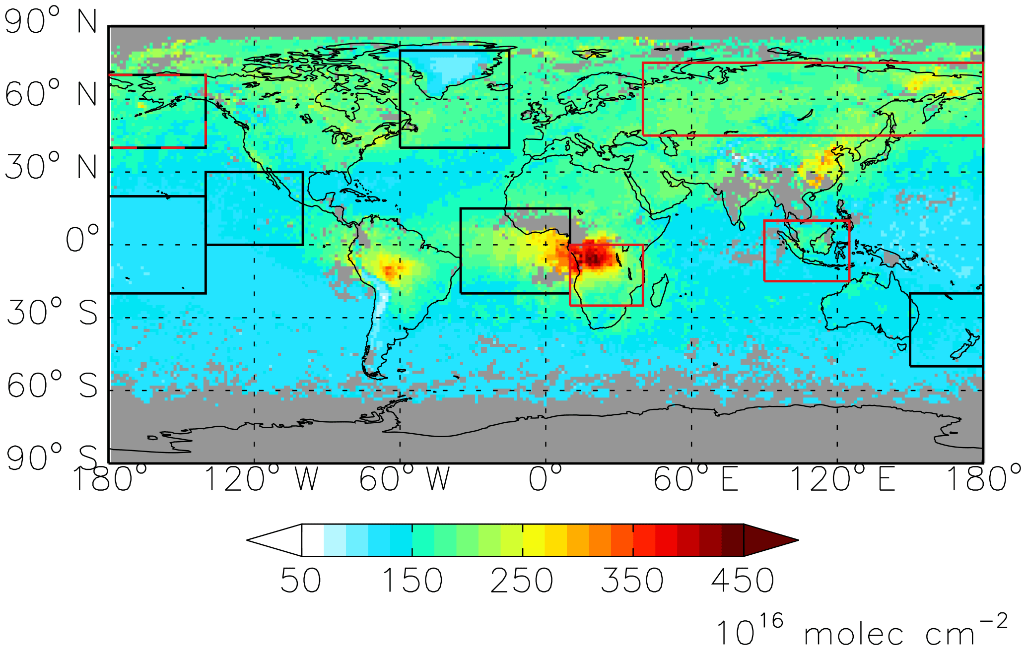
Figure 8MOPITT CO column for August 2016 overplotted with the regions shown in Fig. 10. Black rectangles indicate the regions where we analyze CO concentrations, and red rectangles indicate the regions used for biomass burning.

Figure 9Boxes show the 25th, 50th, and 75th percentile values; whiskers show the minimum and maximum values; black triangles show the mean value; and red circles show the 2016 value for (a) the MOPITT CO column, (b) the GFED4 CO emissions, (c) MOPITT CO at 700 hPa, and (d) MLS CO at 215 hPa. Statistics for MOPITT are for 2000–2016, statistics for GFED4 are for 2000–2015, and statistics for MLS are for 2004–2016. MOPITT and MLS values are for August, while the GFED4 emissions are averaged over June through August.
One of the major goals for the ATom campaign is to produce a climatology based on unbiased, representative samples (Prather et al., 2017). It is therefore important to consider whether August 2016 is a “typical” boreal summer/austral winter month. Prather et al. (2018) found differences of 8–10 % in the chemical reactivity of model-simulated air parcels when considering other years compared to 2016. We focus here on the temporal representativeness of the ATom-1 campaign. August of 2016 was ENSO neutral, with a multivariate ENSO index (MEI) (Wolter and Timlin, 1993) (https://www.esrl.noaa.gov/psd/enso/mei, last access: 9 January 2017) of 0.175 for July/August. However, it was preceded by strong El Niño conditions in 2015 and early 2016 (Blunden and Arndt, 2016). We therefore consider whether the CO concentrations in August 2016 are typical or anomalous.
Multi-year satellite records provide a valuable tool for determining how CO concentrations in the regions of the ATom-1 flights compare to previous years. We focus our analysis of CO interannual variability on several regions traversed by the ATom flights. Figure 8 shows these regions in black squares overplotted on the MOPITT CO column for August 2016. We also examine the IAV in BB sources from nearby regions, outlined in red in Fig. 8. Figure 9 shows box-and-whisker plots of the mean; minimum; 25th, 50th, and 75th percentiles; and maximum in monthly mean August CO for each region over the 2000–2016 period for MOPITT (CO column and CO at 700 hPa) and 2004–2016 for MLS (CO at 215 hPa). The corresponding time series are shown in Fig. 10. The variability in CO BB emissions from the Global Fire Emissions Database version 4 (GFEDv4) (van der Werf et al., 2017) for 2000–2016 is also shown for BB regions that may affect the ATom flights. The BB emissions are averaged over June through August to account for the persistence of CO in the atmosphere.
Among the regions mapped here, the tropical Atlantic shows the highest average CO values, as well as the highest 2016 CO values, in both MOPITT and MLS observations (Fig. 9). This is consistent with large biomass burning emissions from Southern Hemisphere Africa transported into the tropical Atlantic. While Southern Hemisphere Africa has the largest magnitude of biomass burning, its relative variability (variability relative to the mean) is smaller than for the other regions (Fig. 9b). Similarly, the IAV in the MOPITT CO column and 700 hPa level over the tropical Atlantic is smaller than that of the North Atlantic and Alaska regions. Although the variability of CO over the tropical Atlantic is relatively small, the MOPITT CO column shows a statistically significant anti-correlation between the MOPITT CO column over the tropical Atlantic and the MEI (). This relationship is not significant for the MOPITT 700 hPa level.
The time series of August MOPITT CO columns for both the North Atlantic and Alaska, regions that show high variability, show a small but significant temporal correlation with summertime Siberian biomass burning (r=0.52 for the North Atlantic and r=0.59 for Alaska). Slightly lower values are seen for the 700 hPa MOPITT level. The time series of August MOPITT 700 hPa CO shows an increase in 2003 for the North Atlantic and in 2002 and 2003 for Alaska (Fig. 10b, c). Previous studies attribute peaks in these years to the presence of large forest fires in western Russia and Siberia, respectively (Edwards et al., 2004; Yashiro et al., 2009; van der Werf et al., 2006). MOPITT CO values were below average in 2016 for both the North Atlantic and Alaska even though Siberian biomass burning was above average in 2016 (Fig. 9a, b).

Figure 10Time series of August MOPITT CO at the 700 hPa level (black circles) and MLS CO (red triangles) at the 215 hPa level for the six regions shown in black in Fig. 8.
Since ENSO is known to drive large biomass burning variability in Indonesia (van der Werf et al., 2006), we consider whether it may influence CO concentrations over the New Zealand region. Although the MOPITT CO column over the Indonesia region does correlate with the MEI (r=0.64), there is no significant correlation between June–August biomass burning in Indonesia and MOPITT CO over New Zealand. However, August is not the peak season for Indonesian biomass burning (Duncan et al., 2003b). The large Indonesian fires that occurred during the strong 1997/1998 El Niño peaked during September to November (Duncan et al., 2003a), and active fire detections for the 2015 Indonesian fires peaked in September and October (Field et al., 2016). Thus we might expect Indonesian biomass burning variability to have a greater influence on CO variability during the September–October season, which was sampled in ATom-3.
How does 2016 compare to previous years? The MOPITT CO column shows tropical Atlantic CO was near the 75th percentile, while the 700 hPa MOPITT level shows it close to the median. This difference arises because the MOPITT column also includes information from the upper troposphere, and the MOPITT 200 hPa level (not shown) suggests CO levels for 2016 were near the 75th percentile. In contrast, MLS shows that 2016 CO in the upper troposphere was much lower than average, near the 25th percentile. The MOPITT v6 TIR product has a small positive bias drift in the upper troposphere of 0.78 % yr−1 for the 200 hPa level (Deeter et al., 2014), which may contribute to the higher rank of 2016 in the MOPITT upper-tropospheric data compared to MLS. It is therefore hard to argue that 2016 was outside of the normal IAV for this region.
CO in the North Atlantic and Alaska regions in 2016 was below average in both the MOPITT column and the 700 hPa level, and is in fact the lowest August value in the MOPITT record for the 700 hPa level over Alaska. MLS also shows moderately low CO in the upper troposphere over Alaska in August 2016. Combined, these data suggest that the ATom-1 CO is not typical for the region. August 2016 CO column values are also below the median over New Zealand and the eastern and central tropical Pacific, but the relatively low variability of these regions makes this less of a concern for the representativeness of the ATom measurements. The IAV of these regions is larger for the MOPITT 700 hPa level, and 2016 lies slightly below the 25th percentile for this level.
The regionally averaged 500 nm AOT from MODIS (Fig. 11) shows similar features to the MOPITT column. The highest values are found for the tropical Atlantic, followed by the Alaska and North Atlantic regions. This similarity is consistent with the importance of biomass burning emissions for both CO and aerosols. However, the difference between the tropical Atlantic and the other regions is larger in the aerosol case, while the difference between the North Atlantic and the Pacific regions is smaller. There is also greater relative year-to-year variability over the tropical Atlantic for the aerosols than for CO. The shorter lifetime of aerosols compared to CO, as well as the large contribution from biomass burning, likely explains the greater prominence of the tropical Atlantic in the aerosol case. Furthermore, AOT (Fig. 12) shows a clear peak in 2009 in several of the regions, whereas MOPITT data are missing for August 2009, but MLS shows a minimum (tropical Atlantic) or no anomaly (other regions).
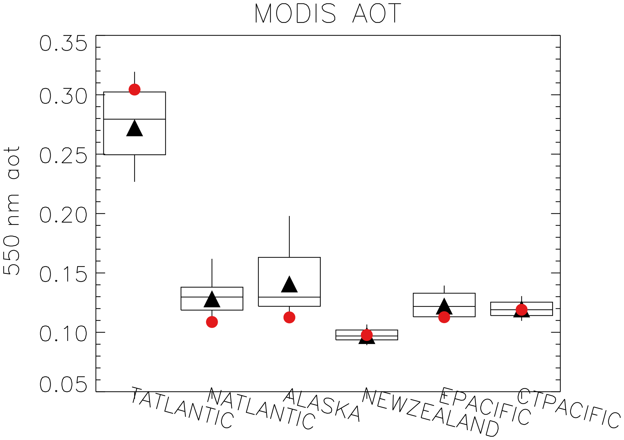
Figure 11As in Fig. 9 but for the August MODIS 550 nm AOT. Only values over oceans are included in the regional averages.
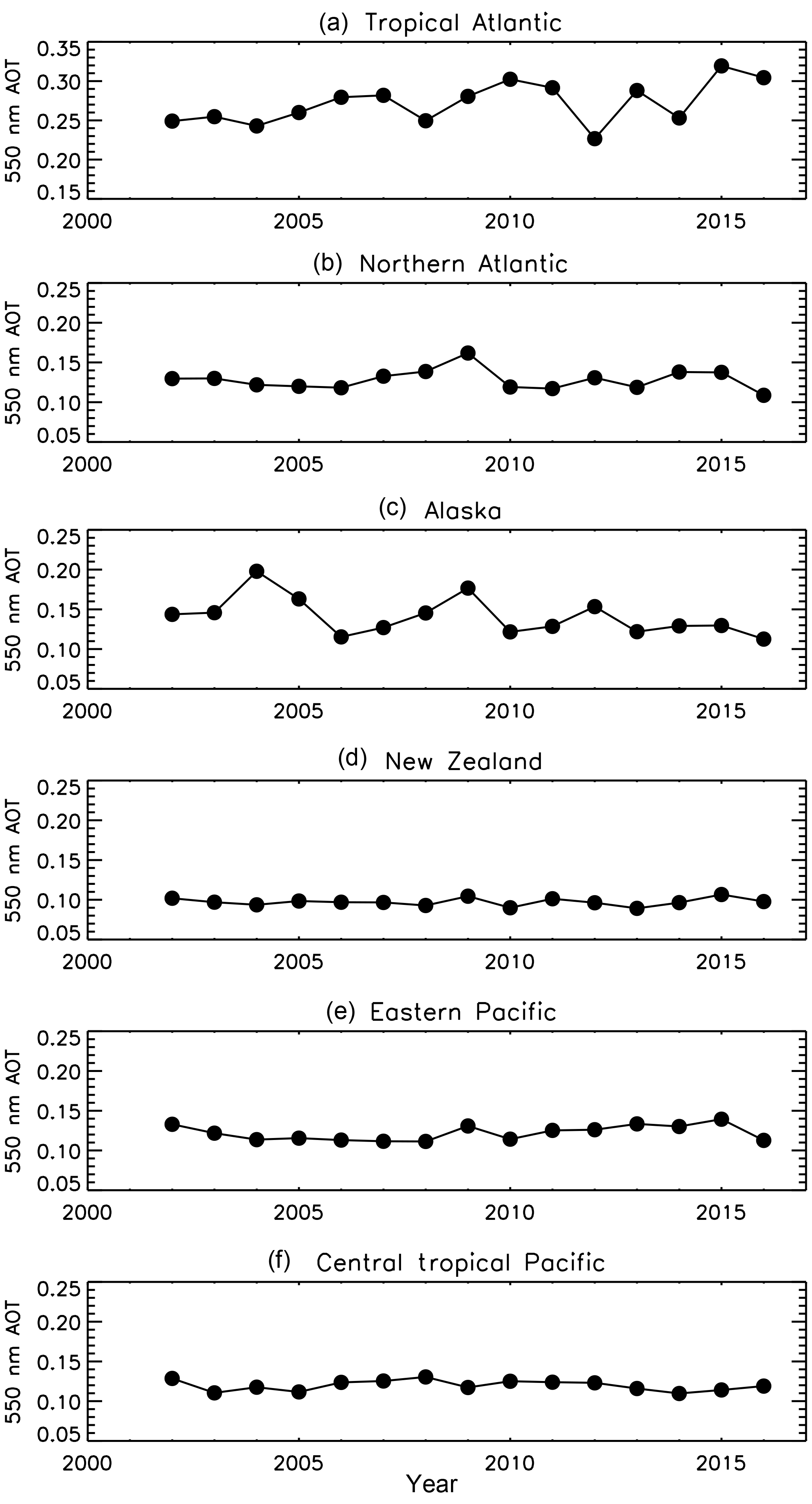
Figure 12Time series of regionally averaged August MODIS 550 nm AOT. Only values over oceans are included in the regional averages. The y-axis range for panel (a) differs from the other panels due to the higher AOT values in that region
In summary, the multi-year satellite record shows considerable variability in CO, particularly over the North Atlantic and Alaska. Concentrations during August 2016 were on the low end of the distribution for most regions, especially in the lower troposphere. Worden et al. (2013) showed negative trends in the MOPITT CO column significant at the 1σ level for both the Northern and Southern Hemisphere for 2000–2012. In addition, Deeter et al. (2014) report a small negative bias drift in the MOPITT V6 TIR product in the lower troposphere, although drift in the column is almost negligible. Decreasing MOPITT CO over time is also visible in some regions in Fig. 10. Overall, the year 2016 shows anomalies for some regions but does not appear to be an extreme year.
We place the observations from the ATom-1 campaign in the context of interannual variability and global source distributions using satellite observations and tagged tracers from GEOS-5, respectively. GEOS-5 gives a reasonable reproduction of the background CO levels for most flights despite the use of climatological fossil fuel and biofuel emissions, and it captures the global distribution of CO observed during ATom-1. Simulations with both forecast and analysis winds capture the timing of many of the enhanced CO plumes encountered during the flights, although the magnitude of the enhancements was often underestimated, which is not unexpected given the difference in resolution between the observations and model. The strong performance of GEOS-5 with regards to the overall CO distribution and the timing of the enhancements gives us confidence in using tagged tracers to identify the sources affecting the air sampled in ATom-1.
We find that for most flights the dominant contribution to total CO is from non-biomass-burning sources, which include both fossil fuels and biofuels and oxidation of hydrocarbons, including methane. An exception to this is in the lower troposphere of the tropical Atlantic, where biomass burning from Africa makes the largest contribution, exceeding 100 ppb in some locations. The non-BB source includes a large fraction from Asia for flights over the North Pacific and from both Asia and North America for the North Atlantic and North American flights, while other regions dominate in the Southern Hemisphere. Plumes of elevated CO from both biomass burning and non-BB sources led to observations of enhanced CO during ATom-1.
We use satellite observations of CO from MOPITT and MLS and AOT from MODIS to assess whether August 2016, the period sampled by ATom-1, is typical or atypical in the context of IAV in the satellite record (2000–2016). MOPITT and MLS show that CO in the lower and upper troposphere, respectively, were below average in August 2016 compared to the satellite record for August for most of the regions sampled by ATom-1, but not usually the minimum year. CO concentrations in the North Atlantic and Alaskan regions show a positive correlation with Siberian biomass burning and large interannual variability. In contrast, both MODIS AOT and the MOPITT CO column show above-average values for the tropical Atlantic in 2016. This suggests that the high values of CO and aerosols from biomass burning encountered during the tropical Atlantic portions of ATom may have been especially pronounced during this particular year.
The seasonality of biomass burning, the OH distribution, and atmospheric transport pathways can alter the source contributions from season to season. Thus, the next three ATom campaigns, which occur in different seasons, will likely show variations in the relative source contributions to each region.
The QCLS data version used in this paper and the corresponding tagged CO model output will be available from the ORNL DAAC at https://doi.org/10.3334/ORNLDAAC/1604 (Strode et al., 2018). MOPITT data are available at https://eosweb.larc.nasa.gov/datapool (MOPITT Science Team, 2013). MLS data are available from https://mls.jpl.nasa.gov/ (Schwartz et al., 2015). MODIS aerosol data are available from https://modis.gsfc.nasa.gov/data/dataprod/mod04.php (Levy et al., 2015).
The supplement related to this article is available online at: https://doi.org/10.5194/acp-18-10955-2018-supplement.
SAS, JL, and LL performed model and data analysis. RC, BD, and SW collected the observations. SW, PN, and MP planned the ATom mission, and LL planned flight paths. AC contributed to the GEOS forecasting. SAS and JL prepared the original manuscript, and all authors contributed to the review and editing of the manuscript.
The authors declare that they have no conflict of interest.
The authors thank the NASA GMAO for providing the GEOS-5 forecasts and
analyses. We thank the NASA Earth Venture Suborbital Program, ESPO, and the
pilots, crew, and support staff of the DC-8.
Edited by: Martyn Chipperfield
Reviewed by: two anonymous
referees
ATom Science Team: NASA Ames Earth Science Project Office (ESPO), available at: https://espoarchive.nasa.gov/archive/browse/atom (last access: 30 July 2018), Moffett Field, CA, 2017.
Bian, H., Colarco, P. R., Chin, M., Chen, G., Rodriguez, J. M., Liang, Q., Blake, D., Chu, D. A., da Silva, A., Darmenov, A. S., Diskin, G., Fuelberg, H. E., Huey, G., Kondo, Y., Nielsen, J. E., Pan, X., and Wisthaler, A.: Source attributions of pollution to the Western Arctic during the NASA ARCTAS field campaign, Atmos. Chem. Phys., 13, 4707–4721, https://doi.org/10.5194/acp-13-4707-2013, 2013.
Blunden, J. and Arndt, D. S. (Eds.): State of the Climate in 2015, B. Am. Meteorol. Soc., 97, S5–S6, 2016.
Darmenov, A. and da Silva, A.: The Quick Fire Emissions Dataset (QFED): Documentation of versions 2.1, 2.2 and 2.4, NASA/TM-2015-104606, Vol. 38, 1–212, 2015.
Deeter, M. N., Martínez-Alonso, S., Edwards, D. P., Emmons, L. K., Gille, J. C., Worden, H. M., Sweeney, C., Pittman, J. V., Daube, B. C., and Wofsy, S. C.: The MOPITT Version 6 product: algorithm enhancements and validation, Atmos. Meas. Tech., 7, 3623–3632, https://doi.org/10.5194/amt-7-3623-2014, 2014.
Duncan, B. N. and Logan, J. A.: Model analysis of the factors regulating the trends and variability of carbon monoxide between 1988 and 1997, Atmos. Chem. Phys., 8, 7389–7403, https://doi.org/10.5194/acp-8-7389-2008, 2008
Duncan, B., Bey, I., Chin, M., Mickley, L., Fairlie, T., Martin, R., and Matsueda, H.: Indonesian wildfires of 1997: Impact on tropospheric chemistry, J. Geophys. Res.-Atmos., 108, 4458, https://doi.org/10.1029/2002JD003195, 2003a.
Duncan, B. N., Martin, R. V., Staudt, A. C., Yevich, R., and Logan, J. A.: Interannual and seasonal variability of biomass burning emissions constrained by satellite observations, J. Geophys. Res.-Atmos., 108, 4100, https://doi.org/10.1029/2002jd002378, 2003b.
Duncan, B. N., Logan, J. A., Bey, I., Megretskaia, I. A., Yantosca, R. M., Novelli, P. C., Jones, N. B., and Rinsland, C. P.: Global budget of CO, 1988–1997: Source estimates and validation with a global model, J. Geophys. Res.-Atmos., 112, 3713–3736, https://doi.org/10.1029/2007JD008459, 2007.
Eastham, S. D. and Jacob, D. J.: Limits on the ability of global Eulerian models to resolve intercontinental transport of chemical plumes, Atmos. Chem. Phys., 17, 2543–2553, https://doi.org/10.5194/acp-17-2543-2017, 2017.
Edwards, D., Petron, G., Novelli, P., Emmons, L., Gille, J., and Drummond, J.: Southern Hemisphere carbon monoxide interannual variability observed by Terra/Measurement of Pollution in the Troposphere (MOPITT), J. Geophys. Res.-Atmos., 111, D16303, https://doi.org/10.1029/2006JD007079, 2006.
Edwards, D. P., Emmons, L. K., Hauglustaine, D. A., Chu, D. A., Gille, J. C., Kaufman, Y. J., Petron, G., Yurganov, L. N., Giglio, L., Deeter, M. N., Yudin, V., Ziskin, D. C., Warner, J., Lamarque, J. F., Francis, G. L., Ho, S. P., Mao, D., Chen, J., Grechko, E. I., and Drummond, J. R.: Observations of carbon monoxide and aerosols from the Terra satellite: Northern Hemisphere variability, J. Geophys. Res.-Atmos., 109, D24202, https://doi.org/10.1029/2004jd004727, 2004.
Emmons, L., Pfister, G., Edwards, D., Gille, J., Sachse, G., Blake, D., Wofsy, S., Gerbig, C., Matross, D., and Nedelec, P.: Measurements of Pollution in the Troposphere (MOPITT) validation exercises during summer 2004 field campaigns over North America, J. Geophys. Res.-Atmos., 112, D12S02, https://doi.org/10.1029/2006JD007833, 2007.
Field, R., van der Werf, G., Fanin, T., Fetzer, E., Fuller, R., Jethva, H., Levy, R., Livesey, N., Luo, M., Torres, O., and Worden, H.: Indonesian fire activity and smoke pollution in 2015 show persistent nonlinear sensitivity to El Nino-induced drought, P. Natl. Acad. Sci. USA, 113, 9204–9209, https://doi.org/10.1073/pnas.1524888113, 2016.
Heald, C., Jacob, D., Fiore, A., Emmons, L., Gille, J., Deeter, M., Warner, J., Edwards, D., Crawford, J., Hamlin, A., Sachse, G., Browell, E., Avery, M., Vay, S., Westberg, D., Blake, D., Singh, H., Sandholm, S., Talbot, R., and Fuelberg, H.: Asian outflow and trans-Pacific transport of carbon monoxide and ozone pollution: An integrated satellite, aircraft, and model perspective, J. Geophys. Res.-Atmos., 108, 4804, https://doi.org/10.1029/2003JD003507, 2003.
Hsu, J., Prather, M., Wild, O., Sundet, J., Isaksen, I., Browell, E., Avery, M., and Sachse, G.: Are the TRACE-P measurements representative of the western Pacific during March 2001?, J. Geophys. Res.-Atmos., 109, D02314, https://doi.org/10.1029/2003JD004002, 2004.
Kasischke, E., Hyer, E., Novelli, P., Bruhwiler, L., French, N., Sukhinin, A., Hewson, J., and Stocks, B.: Influences of boreal fire emissions on Northern Hemisphere atmospheric carbon and carbon monoxide, Global Biogeochem. Cy., 19, GB1012, https://doi.org/10.1029/2004GB002300, 2005.
Langenfelds, R., Francey, R., Pak, B., Steele, L., Lloyd, J., Trudinger, C., and Allison, C.: Interannual growth rate variations of atmospheric CO2 and its δ13C, H2, CH4, and CO between 1992 and 1999 linked to biomass burning, Global Biogeochem. Cy., 16, 1048, https://doi.org/10.1029/2001GB001466, 2002.
Levy, R., Hsu, C., et al.: MODIS Atmosphere L2 Aerosol Product, NASA MODIS Adaptive Processing System, Goddard Space Flight Center, USA, https://doi.org/10.5067/MODIS/MYD04_L2.006, 2015.
Liu, J., Logan, J. A., Murray, L. T., Pumphrey, H. C., Schwartz, M. J., and Megretskaia, I. A.: Transport analysis and source attribution of seasonal and interannual variability of CO in the tropical upper troposphere and lower stratosphere, Atmos. Chem. Phys., 13, 129–146, https://doi.org/10.5194/acp-13-129-2013, 2013.
Livesey, N., Filipiak, M., Froidevaux, L., Read, W., Lambert, A., Santee, M., Jiang, J., Pumphrey, H., Waters, J., Cofield, R., Cuddy, D., Daffer, W., Drouin, B., Fuller, R., Jarnot, R., Jiang, Y., Knosp, B., Li, Q., Perun, V., Schwartz, M., Snyder, W., Stek, P., Thurstans, R., Wagner, P., Avery, M., Browell, E., Cammas, J., Christensen, L., Diskin, G., Gao, R., Jost, H., Loewenstein, M., Lopez, J., Nedelec, P., Osterman, G., Sachse, G., and Webster, C.: Validation of Aura Microwave Limb Sounder O3 and CO observations in the upper troposphere and lower stratosphere, J. Geophys. Res.-Atmos., 113, D15S02, https://doi.org/10.1029/2007JD008805, 2008.
Logan, J., Megretskaia, I., Nassar, R., Murray, L., Zhang, L., Bowman, K., Worden, H., and Luo, M.: Effects of the 2006 El Nino on tropospheric composition as revealed by data from the Tropospheric Emission Spectrometer (TES), Geophys. Res. Lett., 35, L03816, https://doi.org/10.1029/2007GL031698, 2008.
Lucchesi, R: File Specification for GEOS-5 FP, GMAO Office Note No. 4 (Version 1.1), 61 pp., available at: https://gmao.gsfc.nasa.gov/pubs/docs/Lucchesi617.pdf (last access: 31 July 2018), 2017.
Molod, A., Takacs, L., Suarez, M., and Bacmeister, J.: Development of the GEOS-5 atmospheric general circulation model: evolution from MERRA to MERRA2, Geosci. Model Dev., 8, 1339–1356, https://doi.org/10.5194/gmd-8-1339-2015, 2015.
MOPITT Science Team: MOPITT/Terra Level 3 Gridded Monthly CO (on a latitude/longitude/pressure grid) derived from Thermal Infrared Radiances, version 6, Hampton, VA, USA, NASA Atmospheric Science Data Center (ASDC), https://doi.org/10.5067/TERRA/MOPITT/DATA305, 2013.
Novelli, P., Masarie, K., Lang, P., Hall, B., Myers, R., and Elkins, J.: Reanalysis of tropospheric CO trends: Effects of the 1997–1998 wildfires, J. Geophys. Res.-Atmos., 108, 4464, https://doi.org/10.1029/2002JD003031, 2003.
Ott, L., Duncan, B., Pawson, S., Colarco, P., Chin, M., Randles, C., Diehl, T., and Nielsen, E.: Influence of the 2006 Indonesian biomass burning aerosols on tropical dynamics studied with the GEOS-5 AGCM, J. Geophys. Res.-Atmos., 115, D14121, https://doi.org/10.1029/2009jd013181, 2010.
Pfister, G. G., Emmons, L. K., Edwards, D. P., Arellano, A., G Sachse, and Campos, T.: Variability of springtime transpacific pollution transport during 2000–2006: the INTEX-B mission in the context of previous years, Atmos. Chem. Phys., 10, 1345–1359, https://doi.org/10.5194/acp-10-1345-2010, 2010.
Prather, M. J., Zhu, X., Flynn, C. M., Strode, S. A., Rodriguez, J. M., Steenrod, S. D., Liu, J., Lamarque, J.-F., Fiore, A. M., Horowitz, L. W., Mao, J., Murray, L. T., Shindell, D. T., and Wofsy, S. C.: Global atmospheric chemistry – which air matters, Atmos. Chem. Phys., 17, 9081–9102, https://doi.org/10.5194/acp-17-9081-2017, 2017.
Prather, M. J., Flynn, C. M., Zhu, X., Steenrod, S. D., Strode, S. A., Fiore, A. M., Correa, G., Murray, L. T., and Lamarque, J.-F.: How well can global chemistry models calculate the reactivity of short-lived greenhouse gases in the remote troposphere, knowing the chemical composition, Atmos. Meas. Tech., 11, 2653–2668, https://doi.org/10.5194/amt-11-2653-2018, 2018.
Rienecker, M. M., Suarez, M. J., Todling, R., Bacmeister, J., Takacs, L., Liu, H.-C., Gu, W., Sienkiewicz, M., Koster, R. D., Gelaro, R., Stajner, I., and Nielsen, J. E.: The GEOS-5 Data Assimilation System – Documentation of Versions 5.0.1, 5.1.0, and 5.2.0, Technical Report Series on Global Modeling and Data Assimilation, edited by: Suarez, M. J., NASA/TM-2008-104606, Vol. 27, 1–116, 2008.
Rienecker, M. M., Suarez, M. J., Gelaro, R., Todling, R., Bacmeister, J., Liu, E., Bosilovich, M. G., Schubert, S. D., Takacs, L., Kim, G.-K., Bloom, S., Chen, J., Collins, D., Conaty, A., da Silva, A., Gu, W., Joiner, J., Koster, R. D., Lucchesi, R., Molod, A., Owens, T., Pawson, S., Pegion, P., Redder, C. R., Reichle, R., Robertson, F. R., Ruddick, A. G., Sienkiewicz, M., and Woollen, J.: MERRA: NASA's Modern-Era Retrospective Analysis for Research and Applications, J. Climate, 24, 3624–3648, https://doi.org/10.1175/JCLI-D-11-00015.1, 2011.
Santoni, G. W., Daube, B. C., Kort, E. A., Jiménez, R., Park, S., Pittman, J. V., Gottlieb, E., Xiang, B., Zahniser, M. S., Nelson, D. D., McManus, J. B., Peischl, J., Ryerson, T. B., Holloway, J. S., Andrews, A. E., Sweeney, C., Hall, B., Hintsa, E. J., Moore, F. L., Elkins, J. W., Hurst, D. F., Stephens, B. B., Bent, J., and Wofsy, S. C.: Evaluation of the airborne quantum cascade laser spectrometer (QCLS) measurements of the carbon and greenhouse gas suite – CO2, CH4, N2O, and CO – during the CalNex and HIPPO campaigns, Atmos. Meas. Tech., 7, 1509–1526, https://doi.org/10.5194/amt-7-1509-2014, 2014
Schwartz, M., Pumphrey, H., Livesey, N., and Read, W.: MLS/Aura Level 2 Carbon Monoxide (CO) Mixing Ratio V004, Greenbelt, MD, USA, Goddard Earth Sciences Data and Information Services Center (GES DISC), https://doi.org/10.5067/Aura/MLS/DATA2005, 2015.
Strode, S. A. and Pawson, S.: Detection of carbon monoxide trends in the presence of interannual variability, J. Geophys. Res.-Atmos., 118, 12257–12273, https://doi.org/10.1002/2013JD020258, 2013.
Strode, S. A., Liu, J., Lait, L., Commane, R., Daube, B. C., Wofsy, S. C., Conaty A., Newman, P., and Prather, M. J.: ATom: Observed and GEOS-5 Simulated CO Concentrations with Tagged Tracers for ATom-1. ORNL DAAC, Oak Ridge, Tennessee, USA, https://doi.org/10.3334/ORNLDAAC/1604, 2018.
van der Werf, G. R., Randerson, J. T., Giglio, L., Collatz, G. J., Kasibhatla, P. S., and Arellano Jr., A. F.: Interannual variability in global biomass burning emissions from 1997 to 2004, Atmos. Chem. Phys., 6, 3423–3441, https://doi.org/10.5194/acp-6-3423-2006, 2006.
van der Werf, G. R., Randerson, J. T., Giglio, L., van Leeuwen, T. T., Chen, Y., Rogers, B. M., Mu, M., van Marle, M. J. E., Morton, D. C., Collatz, G. J., Yokelson, R. J., and Kasibhatla, P. S.: Global fire emissions estimates during 1997–2016, Earth Syst. Sci. Data, 9, 697–720, https://doi.org/10.5194/essd-9-697-2017, 2017.
Voulgarakis, A., Marlier, M., Faluvegi, G., Shindell, D., Tsigaridis, K., and Mangeon, S.: Interannual variability of tropospheric trace gases and aerosols: The role of biomass burning emissions, J. Geophys. Res.-Atmos., 120, 7157–7173, https://doi.org/10.1002/2014JD022926, 2015.
Waters, J., Froidevaux, L., Harwood, R., Jarnot, R., Pickett, H., Read, W., Siegel, P., Cofield, R., Filipiak, M., Flower, D., Holden, J., Lau, G., Livesey, N., Manney, G., Pumphrey, H., Santee, M., Wu, D., Cuddy, D., Lay, R., Loo, M., Perun, V., Schwartz, M., Stek, P., Thurstans, R., Boyles, M., Chandra, K., Chavez, M., Chen, G., Chudasama, B., Dodge, R., Fuller, R., Girard, M., Jiang, J., Jiang, Y., Knosp, B., LaBelle, R., Lam, J., Lee, K., Miller, D., Oswald, J., Patel, N., Pukala, D., Quintero, O., Scaff, D., Van Snyder, W., Tope, M., Wagner, P., and Walch, M.: The Earth Observing System Microwave Limb Sounder (EOS MLS) on the Aura satellite, IEEE T. Geosci. Remote, 44, 1075–1092, https://doi.org/10.1109/TGRS.2006.873771, 2006.
Wofsy, S. C., Apel, E., Blake, D. R., Brock, C. A., Brune, W. H., Bui, T. P., Daube, B. C., Dibb, J. E., Diskin, G. S., Elkiins, J. W., Froyd, K., Hall, S. R., Hanisco, T. F., Huey, L. G., Jimenez, J. L., McKain, K., Montzka, S. A., Ryerson, T. B., Schwarz, J. P., Stephens, B. B., Weinzierl, B., and Wennberg, P.: ATom: Merged Atmospheric Chemistry, Trace Gases, and Aerosols, ORNL DAAC, Oak Ridge, Tennessee, USA, https://doi.org/10.3334/ORNLDAAC/1581, 2018.
Wolter, K. and Timlin, M. S.: Monitoring ENSO in COADS with a seasonally adjusted principal component index, Proc. of the 17th Climate Diagnostics Workshop, Norman, OK, USA, 1993.
Worden, H. M., Deeter, M. N., Frankenberg, C., George, M., Nichitiu, F., Worden, J., Aben, I., Bowman, K. W., Clerbaux, C., Coheur, P. F., de Laat, A. T. J., Detweiler, R., Drummond, J. R., Edwards, D. P., Gille, J. C., Hurtmans, D., Luo, M., Martínez-Alonso, S., Massie, S., Pfister, G., and Warner, J. X.: Decadal record of satellite carbon monoxide observations, Atmos. Chem. Phys., 13, 837–850, https://doi.org/10.5194/acp-13-837-2013, 2013.
Yashiro, H., Sugawara, S., Sudo, K., Aoki, S., and Nakazawa, T.: Temporal and spatial variations of carbon monoxide over the western part of the Pacific Ocean, J. Geophys. Res.-Atmos., 114, D08305, https://doi.org/10.1029/2008JD010876, 2009.
Ziemke, J. and Chandra, S.: La Nina and El Nino-induced variabilities of ozone in the tropical lower atmosphere during 1970–2001, Geophys. Res. Lett., 30, 1142, https://doi.org/10.1029/2002GL016387, 2003.
- Abstract
- Introduction
- Observations and model
- GEOS-5 chemical forecasting for ATom
- Source contributions to the global CO distribution
- August 2016 in the context of interannual variability (IAV)
- Conclusions
- Data availability
- Author contributions
- Competing interests
- Acknowledgements
- References
- Supplement