the Creative Commons Attribution 4.0 License.
the Creative Commons Attribution 4.0 License.
 | 03 Aug 2018
Polar stratospheric cloud climatology based on CALIPSO spaceborne lidar measurements from 2006 to 2017
Michael C. Pitts
Lamont R. Poole
Ryan Gonzalez
The Cloud-Aerosol Lidar with Orthogonal Polarization (CALIOP) on the CALIPSO (Cloud-Aerosol Lidar and Infrared Pathfinder Satellite Observations) satellite has been observing polar stratospheric clouds (PSCs) from mid-June 2006 until the present. The spaceborne lidar profiles PSCs with unprecedented spatial (5 km horizontal×180 m vertical) resolution and its dual-polarization capability enables classification of PSCs according to composition. Nearly coincident Aura Microwave Limb Sounder (MLS) measurements of the primary PSC condensables (HNO3 and H2O) provide additional constraints on particle composition. A new CALIOP version 2 (v2) PSC detection and composition classification algorithm has been implemented that corrects known deficiencies in previous algorithms and includes additional refinements to improve composition discrimination. Major v2 enhancements include dynamic adjustment of composition boundaries to account for effects of denitrification and dehydration, explicit use of measurement uncertainties, addition of composition confidence indices, and retrieval of particulate backscatter, which enables simplified estimates of particulate surface area density (SAD) and volume density (VD). The over 11 years of CALIOP PSC observations in each v2 composition class conform to their expected thermodynamic existence regimes, which is consistent with previous analyses of data from 2006 to 2011 and underscores the robustness of the v2 composition discrimination approach.
The v2 algorithm has been applied to the CALIOP dataset to produce a PSC reference data record spanning the 2006–2017 time period, which is the foundation for a new comprehensive, high-resolution climatology of PSC occurrence and composition for both the Antarctic and Arctic. Time series of daily-averaged, vortex-wide PSC areal coverage versus altitude illustrate that Antarctic PSC seasons are similar from year to year, with about 25 % relative standard deviation in Antarctic PSC spatial volume at the peak of the season in July and August. Multi-year average, monthly zonal mean cross sections depict the climatological patterns of Antarctic PSC occurrence in latitude–altitude and also equivalent-latitude–potential-temperature coordinate systems, with the latter system better capturing the microphysical processes controlling PSC existence. Polar maps of the multi-year mean geographical patterns in PSC occurrence frequency show a climatological maximum between longitudes 90∘ W and 0∘, which is the preferential region for forcing by orography and upper tropospheric anticyclones. The climatological mean distributions of particulate SAD and VD also show maxima in this region due to the large enhancements from the frequent ice clouds.
Stronger wave activity in the Northern Hemisphere leads to a more disturbed Arctic polar vortex, whose evolution and lifetime vary significantly from year to year. Accordingly, Arctic PSC areal coverage is distinct from year to year with no “typical” year, and the relative standard deviation in Arctic PSC spatial volume is >100 % throughout most of the season. When PSCs are present in the Arctic, they most likely occur between longitudes 60∘ W and 90∘ E, which is consistent with the preferential location of the Arctic vortex.
Comparisons of CALIOP v2 and Michelson Interferometer for Passive Atmospheric Sounding (MIPAS) Antarctic PSC observations show excellent correspondence in the overall spatial and temporal evolution, as well as for different PSC composition classes. Climatological patterns of CALIOP v2 PSC occurrence frequency in the vicinity of McMurdo Station, Antarctica, and Ny-Ålesund, Spitsbergen, are similar in nature to those derived from local ground-based lidar measurements. To investigate the possibility of longer-term trends, appropriately subsampled and averaged CALIOP v2 PSC observations from 2006 to 2017 were compared with PSC data during the 1978–1989 period obtained by the spaceborne solar occultation instrument SAM II (Stratospheric Aerosol Measurement II). There was good consistency between the two instruments in column Antarctic PSC occurrence frequency, suggesting that there has been no long-term trend. There was less overall consistency between the Arctic records, but it is very likely due to the high degree of interannual variability in PSCs rather than a long-term trend.


The overall role of polar stratospheric clouds (PSCs) in the depletion of stratospheric ozone is well established (Solomon, 1999). Heterogeneous reactions on PSC particles convert the stable chlorine reservoirs HCl and ClONO2 to chlorine radicals that destroy ozone catalytically (Solomon et al., 1986; Crutzen et al., 1992; Solomon, 1999). Rates of these reactions depend on particle surface area density (SAD) and composition, which can include binary (H2SO4–H2O) or ternary (HNO3–H2SO4–H2O, or STS, supercooled ternary solution) liquid droplets, solid nitric acid trihydrate (NAT) particles, and H2O ice particles (Lowe and MacKenzie, 2008). PSCs also impact polar ozone chemistry by temporarily removing gas-phase HNO3 from the polar stratosphere through uptake by the particles during formation and growth (denoxification). In addition, sedimentation of large NAT particles (Fahey et al., 2001; Northway et al., 2002; Molleker et al., 2014) can permanently remove HNO3 (denitrification), which prolongs ozone depletion by delaying reformation of the stable chlorine reservoirs. A substantial recovery of the ozone layer is expected by the middle of this century with reduced global production of ozone depleting substances in accordance with the Montreal Protocol and subsequent amendments and adjustments (WMO (World Meteorological Organization), 2015). But as climate changes, leading to a colder and perhaps wetter stratosphere and upper troposphere (e.g., Shindell, 2001), reliable model predictions of recovery of the Antarctic ozone hole and of potentially more severe ozone depletion in the Arctic are challenging because many global models use simple parameterizations that do not accurately represent PSC processes (e.g., Peter and Grooß, 2012; Morgenstern et al., 2017).
Fortunately, our knowledge of the temporal and geographic distribution of PSCs and their particle composition has expanded greatly in the 21st century with the advent of three satellite instruments with extensive polar measurement coverage: the Michelson Interferometer for Passive Atmospheric Sounding (MIPAS) on Envisat (2002–2012), the Microwave Limb Sounder (MLS) on Aura (2004–present), and the Cloud-Aerosol Lidar with Orthogonal Polarization (CALIOP) on CALIPSO (Cloud-Aerosol Lidar and Infrared Pathfinder Satellite Observations, 2006–present). CALIPSO flies in a 98∘ inclination orbit at an altitude of 705 km as part of the NASA A-train satellite constellation (Stephens et al., 2002), along with the Aqua, Aura, CloudSat, and Orbiting Carbon Observatory 2 (OCO-2) satellites. Although PSC studies are not a primary mission objective, CALIPSO is an ideal platform for studying polar processes, collecting data along 14–15 orbits per day with coverage from 82∘ S to 82∘ N latitude on each orbit. CALIOP data collection began in mid-June 2006 and continues at the time of this writing.
The foundation for PSC detection and composition classification using CALIOP data was laid out in papers by Pitts et al. (2007, 2009), with additional refinements appearing in Pitts et al. (2011, 2013). We will refer to these papers herein as P07, P09, P11, and P13, respectively, and refer to the P07/P09/P11/P13 algorithm sequence as version 1.0 (v1). Data products from v1 have compared favorably with PSC observations from MIPAS (Höpfner et al., 2009), ground-based lidar (Achtert and Tesche, 2014), and Aura MLS (P13; Lambert et al., 2016). However, several known deficiencies in the v1 algorithm were highlighted in P13, one being that the effects of measurement noise on the inferred PSC composition were not explicitly considered. In addition, the boundary separating NAT and ice PSCs in the CALIOP optical measurement space needed to be adjusted in the event of denitrification and dehydration – a shortcoming that was also noted in comparisons of v1 products with model simulations by Zhu et al. (2017).
In the present paper, we introduce the CALIOP version 2.0 (v2) PSC algorithm, which addresses these known deficiencies and includes additional refinements to increase the robustness of the inferred PSC composition. These refinements include (1) correction for crosstalk between the CALIOP parallel and perpendicular polarization channels; (2) estimation of random uncertainties in the measured and derived optical quantities using the noise-scale factor approach (Liu et al., 2006); (3) adoption of less conservative PSC detection thresholds to better match features detected by the naked eye in CALIOP orbital curtain images; (4) redefined PSC composition classes with indices denoting statistical confidence in the inferred composition; and (5) retrieval of 532 nm particulate backscatter, which corrects the CALIOP measurements for attenuation by overlying particle layers and enables simplified estimates of the bulk particle microphysical quantities SAD and volume density (VD) to facilitate comparisons with PSC measurements by other instruments as well as with theoretical model representations of heterogeneous chemical processes. We show several examples that illustrate the top-level differences between v1 and v2 data products. We then present a state-of-the-art PSC reference data record and climatology constructed by applying the v2 algorithm to the over 11 years of CALIOP spaceborne lidar data spanning 2006 to 2017. This work is part of a larger effort to compile new reference PSC climatologies based on the contemporary CALIOP, MIPAS, and MLS datasets that is being performed under the auspices of the Stratosphere-troposphere Processes And their Role in Climate (SPARC) Polar Stratospheric Cloud Initiative (PSCi: http://www.sparc-climate.org/activities/polar-stratospheric-clouds/, last access: June 2018). A separate MIPAS PSC climatology has been compiled by Spang et al. (2018). These new climatologies represent the first observation-based records of PSC occurrence, composition, and particle characteristics on vortex-wide spatial scales covering decadal timescales and are a valuable resource for testing and validating current and future global models.
In Sect. 2 we describe the datasets utilized in the CALIOP v2 PSC algorithm and in constructing the CALIOP PSC climatology. In Sect. 3 we describe in detail the modifications implemented in the v2 algorithm, illustrate the top-level differences between v1 and v2, and show that the v2 PSC composition classes conform well to their expected temperature existence regimes. In Sect. 4 we present the CALIOP v2 PSC reference data record and climatology in terms of overall and composition-specific areal coverage and occurrence frequency. Multi-year average, monthly zonal mean cross sections in both latitude–altitude and equivalent-latitude–potential-temperature coordinate systems are shown along with polar maps that illustrate the detailed temporal and spatial patterns in PSC occurrence and composition. In Sect. 5 we show examples of the SAD climatology. In Sect. 6 we discuss comparisons of CALIOP with MIPAS and ground-based lidar PSC observations and investigate the possibility of long-term trends in PSC occurrence by comparing the CALIOP data record to the historical (1978–1989) SAM II (Stratospheric Aerosol Measurement II) solar occultation PSC occurrence record. Finally, in Sect. 7 we summarize the key findings and discuss the results.
The A-train satellite constellation offers a unique opportunity for PSC analyses through the combination of CALIOP data and nearly coincident Aura MLS measurements of the primary PSC condensable vapors, HNO3 and H2O. Additional context is provided by ancillary meteorological information from the Modern-Era Retrospective analysis for Research and Applications (MERRA-2) reanalysis products (Gelaro et al., 2017) and the Aura MLS derived meteorological products (DMPs) (Manney et al., 2007, 2011a). A brief description of these datasets is provided below.
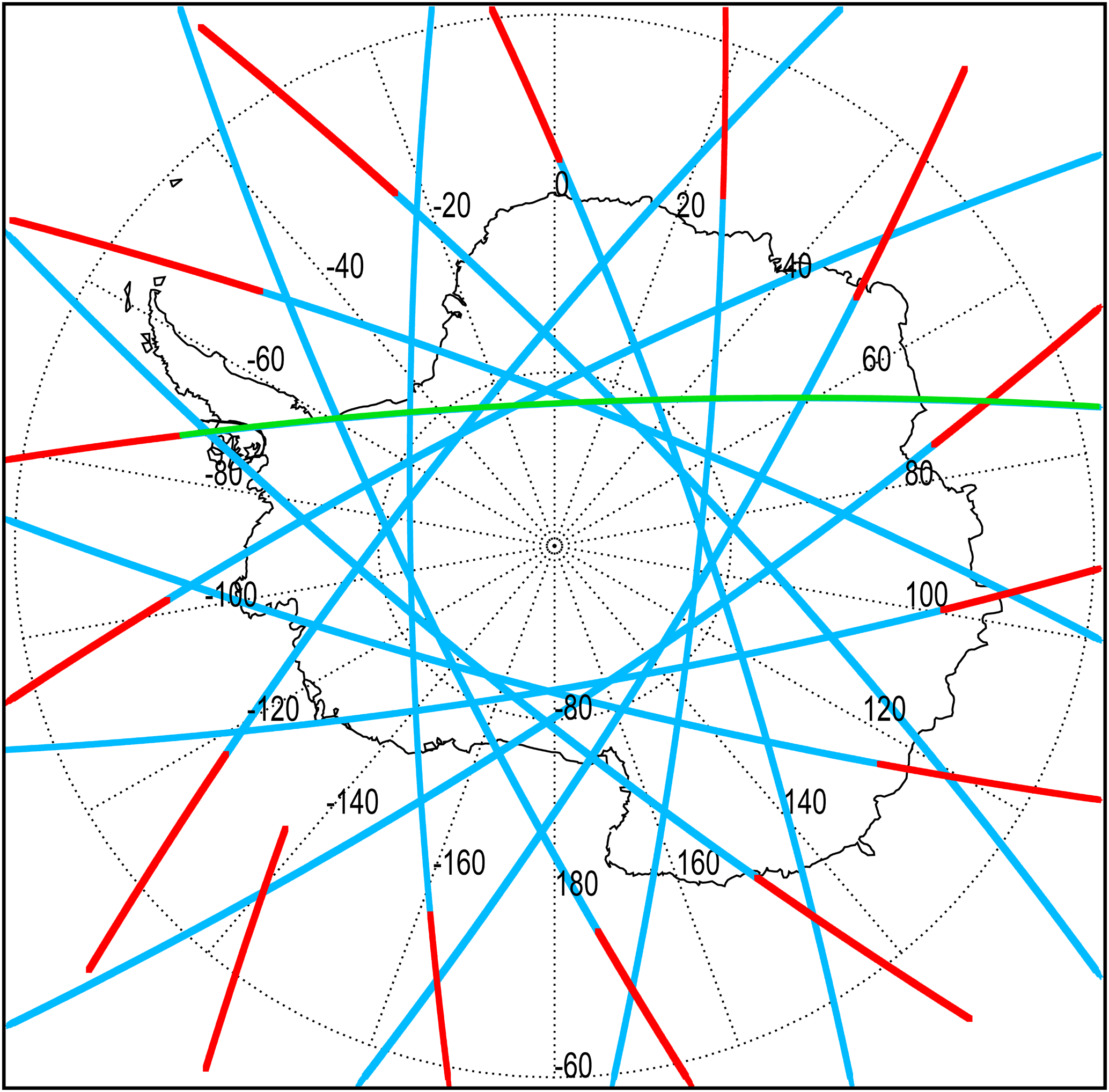
Figure 1CALIPSO orbital coverage over the polar region of the Southern Hemisphere on 17 July 2008. Blue (red) lines depict nighttime (daytime) orbit segments. The CALIOP curtain along the orbit highlighted in green is shown in Fig. 2.
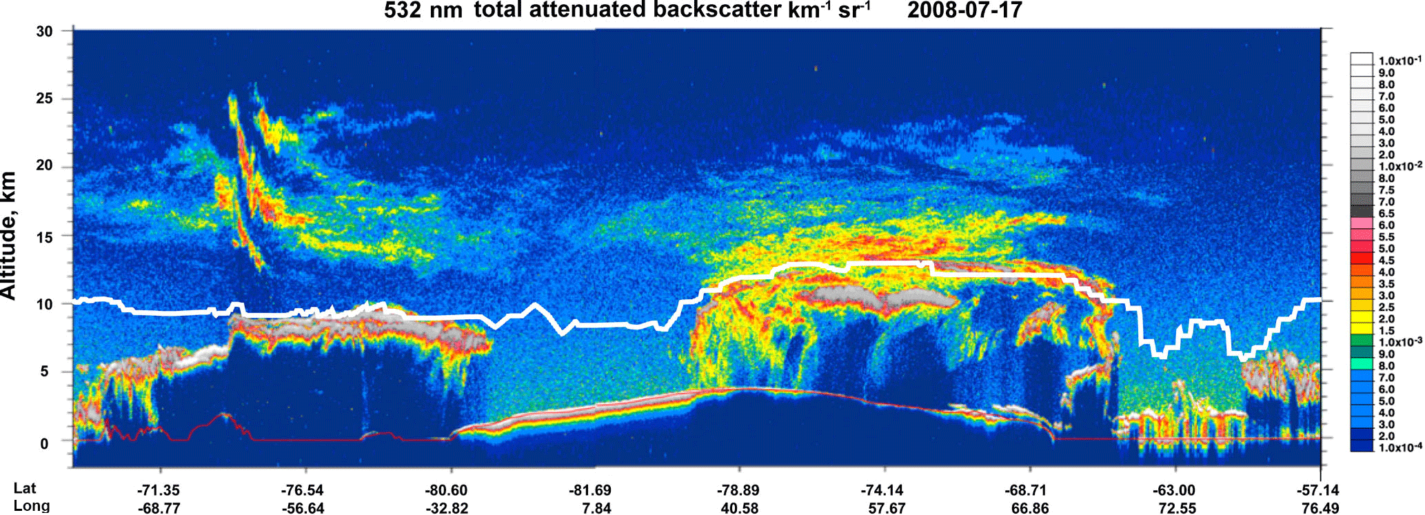
Figure 2Orbital curtain of CALIOP 532 nm total attenuated backscatter coefficient () along the single orbit highlighted in green in Fig. 1. The MERRA-2 tropopause height is indicated by the solid white line.
2.1 CALIOP
CALIOP, the primary instrument on the CALIPSO satellite, is a dual-wavelength polarization-sensitive lidar that provides high-vertical-resolution profiles of backscatter coefficients at 532 and 1064 nm (Winker et al., 2009). Figure 1 illustrates the typical CALIPSO orbital coverage for a single day (17 July 2008) over the Antarctic polar region. A curtain of CALIOP 532 nm total attenuated backscatter coefficient measurements along a single orbit from this day is shown in Fig. 2 and illustrates the unique capability of the CALIOP spaceborne lidar to probe clouds and aerosols at very high spatial resolution. Although not specifically designed for stratospheric applications, PSCs generally produce detectable enhancements in CALIOP backscatter profiles as can be seen at altitudes above ∼12 km along the orbit curtain in Fig. 2. The CALIOP measurements of the 532 nm perpendicular backscatter coefficient provide additional information on particle shape, from which PSC composition can be inferred. The v2 CALIOP PSC data products are derived from nighttime-only CALIOP v4.10 level 1B 532 nm parallel and perpendicular backscatter coefficient measurements; daytime measurements contain elevated background noise due to scattered sunlight, which greatly inhibits the detection of PSCs. Ancillary meteorological data from MERRA-2, including temperature, pressure, ozone number density, and tropopause height at the CALIOP measurement locations, are included in the CALIOP v4.10 level 1B data products and utilized in the PSC algorithm as described in Sect. 3. Further details on the CALIPSO v4.10 level 1 data processing and calibration approach can be found in Kar et al. (2018).
2.2 Aura MLS
The Aura satellite flies in formation with CALIPSO in the A-train satellite constellation providing a nearly coincident dataset of gas-phase HNO3 and H2O from the MLS instrument with spatial and temporal differences between the CALIOP and MLS measurements less than 10 km and 30 s after a repositioning of the Aura satellite in April 2008 and about 200 km and 7–8 min prior to 2008 (see Lambert et al., 2012). The Aura MLS detects thermal microwave emission from the Earth's limb along the line of sight in the forward direction of the Aura spacecraft flight track (Waters et al., 2006). Vertical scans are made from the Earth's surface up to a 90 km tangent height every 24.7 s, providing a total of 3500 vertical profiles per day with a horizontal along-track spacing of 1.5∘ (∼165 km) and nearly global latitude coverage from 82∘ S to 82∘ N. The limb radiance measurements are inverted using a 2-D optimal estimation retrieval (Livesey et al., 2006) to yield atmospheric profiles of temperature and gas-phase constituents in the vertical range 8–90 km. Herein we use the MLS version 4.2 products (Livesey et al., 2017). For the vertical range relevant for PSCs, the MLS version 4.2 measurements have typical single-profile precisions (accuracies) of 4–15 % (4–7 %) for H2O (Read et al., 2007; Lambert et al., 2007) and 0.6 ppbv (1–2 ppbv) for HNO3 (Santee et al., 2007). Vertical and horizontal along-track resolutions are 3.1–3.5 and 180–290 km for H2O, and 3.5–5.5 and 400–550 km for HNO3.
The Aura MLS version 2 (v2) derived meteorological products (Manney et al., 2007, 2011a) have been calculated from the MERRA-2 reanalyses and consist of meteorological variables (winds, temperature, potential temperature, potential vorticity) and derived fields (e.g., equivalent latitude and vortex edge location) interpolated to the locations and times of the Aura MLS observations.
To better facilitate the utilization of the MLS data in the PSC analyses, the MLS gas-phase HNO3 and H2O measurements are interpolated to the CALIOP PSC orbit grid using an average of the two nearest MLS profiles weighted by the inverse of the relative distance of each to the CALIPSO locations. In addition, meteorological parameters from the Aura MLS v2.0 DMPs are also mapped onto the CALIOP PSC orbit grid. The MLS HNO3 and H2O and the meteorological parameters from the DMPs are included in the archived v2 CALIOP PSC data product files.
3.1 Data preprocessing
Data preprocessing generally follows the procedure discussed in detail in P07 and P09, but with additional steps (see Appendix A) to correct for the small amount of crosstalk between the two CALIOP polarization channels and to estimate uncertainties [u(x)] in the basic CALIOP measurements and derived quantities. The initial step is to ingest nighttime-only profiles of CALIOP v4.10 lidar level 1B 532 nm attenuated parallel () and perpendicular () backscatter coefficients over the altitude range 8.4–30 km. The data are smoothed to a uniform 5 km horizontal (along the orbit track) by 180 m vertical resolution grid to remove the altitude dependence of the resolution of the downlinked CALIOP data (Winker et al., 2007). The data are then corrected for molecular and ozone attenuation using the MERRA-2 molecular and ozone number density profiles reported in the CALIOP v4.10 level 1B data product files. The MERRA-2 molecular number density is also used in the theoretical relationship from Hostetler et al. (2006) to calculate molecular backscatter βmol, which is then used to calculate the 532 nm attenuated scattering ratio
3.2 PSC detection
Detection of PSCs in the v2 algorithm generally follows the approach of v1 in that PSCs are detected as statistical outliers in either or relative to the background stratospheric aerosol population. We also use successive horizontal averaging (5, 15, 45, and 135 km) to ensure that strongly scattering PSCs (e.g., fully developed STS and ice) are found at the finest possible spatial resolution while also enabling the detection of more tenuous PSCs (e.g., low number density liquid–NAT mixtures) through additional averaging. PSC features found at finer spatial resolution are masked out of the profiles of and that undergo additional averaging. Successive averaging minimizes optical aliasing that can result from grouping fine-resolution pixels having vastly different optical properties into a single coarser-resolution average.
Visual comparison of many CALIOP v1 orbital composition images (e.g., Fig. 13 of P11) with corresponding images of and indicated that the PSC statistical thresholds used in the v1 algorithm were too conservative, so we have made appropriate adjustments in v2. The thresholds for the background aerosol – assumed to be those data at MERRA-2 temperatures above 200 K – are now defined as the daily median plus one median absolute deviation of and . These are computed in overlapping 100 K thick potential temperature (θ) layers over the range from θ=250–750 K. The region of the South Atlantic Anomaly, defined here as a wedge between longitudes 60∘ W and 45∘ E, is excluded from the background aerosol threshold calculations due to excessive noise in the CALIOP 532 nm data in this region (Hunt et al., 2009). Then for a candidate CALIOP data point to be identified as a PSC, its value of (or ) must exceed the background aerosol threshold by at least (or ). We also impose a spatial coherence test that requires that more than 11 of the points in a 5-point horizontal by 3-point vertical box centered on the candidate feature exceed the current PSC detection threshold or have been identified as a PSC at a previous (finer) averaging scale. This revised approach does a better job overall of capturing PSC clusters identified by the naked eye in CALIOP orbital images while continuing to eliminate false PSC identifications stemming from positive noise spikes in the data. Spot checks of the v2 Antarctic PSC database from early May – when no PSCs observations are expected – indicate that the v2 false positive rate is much less than 0.01 %.
Tropopause height information included in the CALIOP v4.10 level 1b lidar data product files is based on the MERRA-2 “blended” tropopause altitudes. The MERRA-2 blended tropopause is the lower (in altitude) of the temperature-based (“thermal”) tropopause and potential vorticity (PV)-based (“dynamic”) tropopause (Bosilovich et al., 2016; Ott et al., 2016). In practice, the MERRA-2 blended tropopause is usually the dynamic tropopause in mid- and high latitudes, but switches to the thermal tropopause in the tropics. The tropopause is often difficult to locate in the polar regions, especially during the polar nights (e.g., Highwood et al., 2000), so any tropopause height determination in these regions should be used with caution. In fact, it is our experience that the transition from upper tropospheric cirrus to PSCs is often ambiguous with no clear separation across the reported tropopause. Consequently, using the MERRA-2 tropopause as a hard boundary to separate tropospheric cirrus from PSCs will certainly lead to misclassifications. Hence, we make no explicit attempt to distinguish tropospheric cloud from stratospheric cloud in the 8.5–30 km altitude range over which we produce the CALIOP PSC cloud mask. However, we do tag each observation in the database with a feature flag that identifies its altitude location relative to the reported blended tropopause as one of three possibilities: (1) below the tropopause, (2) between the tropopause and tropopause +4 km, or (3) above the tropopause +4 km. This allows data users to perform some crude separation between tropospheric and stratospheric cloud as desired.
3.3 PSC composition classification
PSC composition classification is based on comparing CALIOP data with temperature-dependent theoretical optical calculations for non-equilibrium mixtures of liquid (binary H2SO4–H2O or STS) droplets and NAT or ice particles. To illustrate the differences between the v2 and v1 algorithms, we show a more extensive set of theoretical results for 50 hPa atmospheric pressure, 10 ppbv HNO3, and 5 ppmv H2O. For these conditions, the NAT equilibrium temperature TNAT≅195.7 K (Hanson and Mauersberger, 1988); the temperature at which liquid particle volume starts to increase markedly TSTS≅192 K (Carslaw et al., 1995); and the frost point temperature, Tice≅188.5 K (Murphy and Koop, 2005). The total particle number density (Ntotal) is fixed at 10 cm−3 (Weigel et al., 2014), partitioned between liquid droplets (Nliq) and either NAT (NNAT) or ice (Nice) for the various mixtures being considered. The liquid particle size distribution is assumed to be a single-mode lognormal with geometric standard deviation σ=1.6, whose mode radius is calculated as a function of Nliq and the equilibrium condensed liquid particle VD (Carslaw et al., 1995) for temperatures . We assume that non-equilibrium liquid–NAT mixtures exist at T<TNAT and that non-equilibrium liquid–ice mixtures exist at T<Tice and that both NAT and ice particle size distributions are single-mode lognormals with σ=1.38. We consider a range of NNAT(Nice) from 0.0001 to 1.0 cm−3 (0.001 to 10 cm−3) and a range of volume-equivalent radii (rNAT and rice) from 0.25 to 15 µm. However, only those combinations of [N, r] with NAT (ice) particle volumes less than or equal to the temperature-dependent equilibrium NAT (ice) volume are physically possible. For the liquid–NAT mixtures, , and the equilibrium liquid particle VD is reduced to account for the condensed HNO3 and H2O in the coexisting NAT particles. For the liquid–ice mixtures, , and the equilibrium liquid particle VD is reduced to account for the condensed H2O in the coexisting ice particles. All particle optical properties were calculated using the database of T-matrix results compiled by Scarchilli et al. (2005) and based on the original work of Mishchenko and Travis (1998), with fixed refractive indices of 1.44+i0.0 for binary H2SO4–H2O and STS, 1.48+i0.0 for NAT, and 1.31+i0.0 for ice. We assumed spherical liquid droplets (aspect ratio=1.0) and assumed both NAT and ice particles to be prolate spheroids with an aspect (diameter-to-length) ratio of 0.9, which Engel et al. (2013) showed to produce the best agreement with maximum values observed by CALIOP of particulate depolarization ratio δparticulate:
where δmol is the theoretical molecular depolarization ratio =0.00366 (see Appendix A).
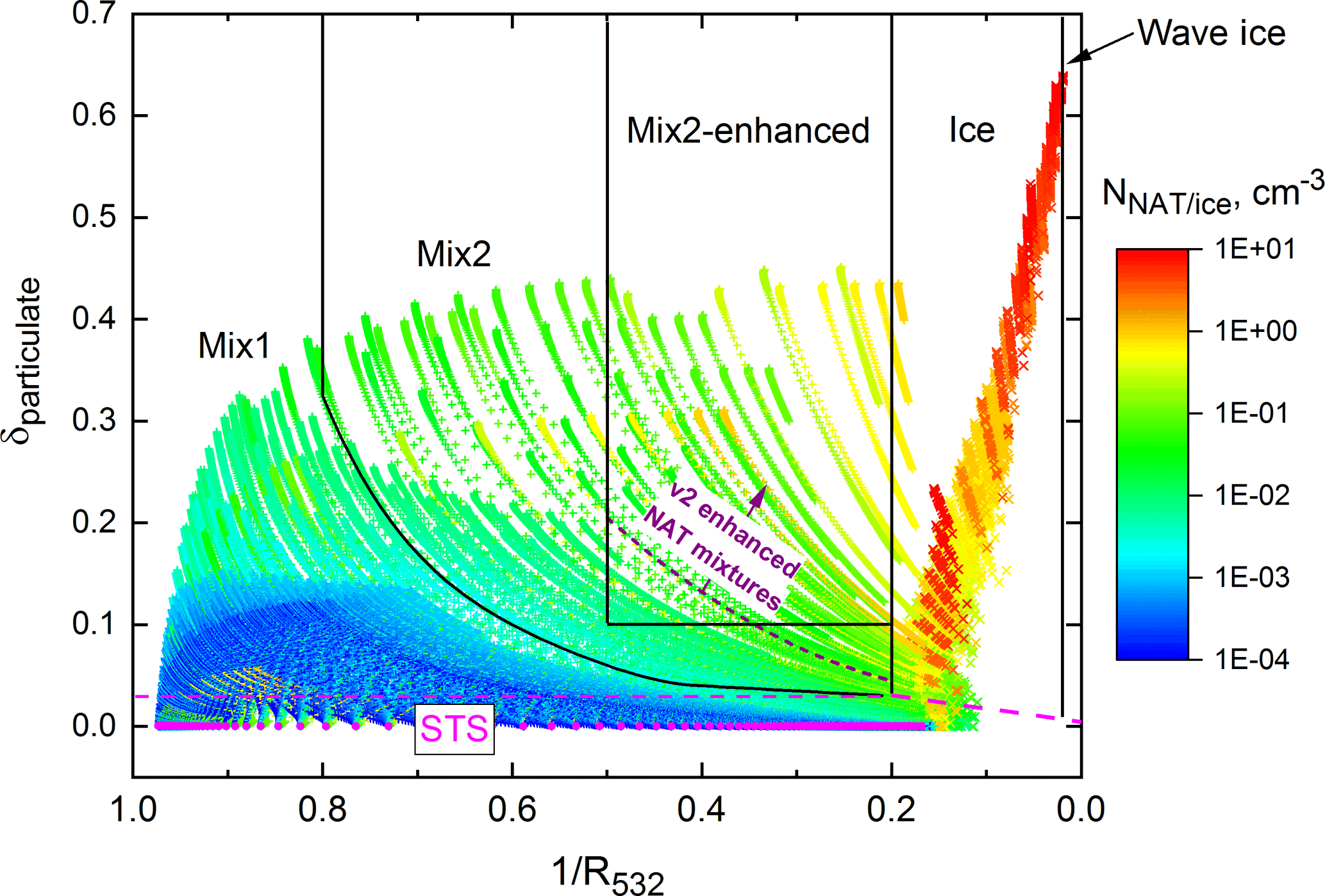
Figure 3Theoretical optical calculations for non-equilibrium liquid–NAT and liquid–ice mixtures, illustrating the v1 PSC composition classification scheme. The dashed purple curve represents the lower boundary of the v2 enhanced NAT mixtures composition class, as discussed in the text and in Fig. 4.
Figure 3 shows the theoretical results plotted in the coordinate system of δparticulate vs. inverse scattering ratio (1∕R532) used in the v1 algorithm. In v1, it was assumed implicitly that attenuation of the CALIOP laser beam due to PSC particles themselves was negligible, i.e., that and could be considered equivalent to R532 and β⊥ for the purpose of composition classification. The individual “streaks” of points in Fig. 3 represent physically possible [NNAT, rNAT] or [Nice, rice] combinations, with temperature decreasing from upper left to lower right along each streak. P09 defined fixed δparticulate vs. 1∕R532 boundaries separating the composition classes STS, ice (our abbreviated name for liquid–ice mixtures), and Mix1 and Mix2, with the latter denoting liquid–NAT mixtures with lower and higher NAT number densities and volumes, respectively. P11 added two additional subclasses: Mix2 enhanced, those liquid–NAT mixtures with optical properties ( and δparticulate>0.1) similar to the so-called type 1a enhanced clouds observed during earlier airborne field missions (e.g., Tsias et al., 1999); and wave ice, which are PSCs presumably induced by mountain waves. P11 defined wave ice conservatively as those PSCs with R532>50, but noted that the subclass is not all-inclusive; i.e., some additional ice PSCs are likely associated with mountain waves, but do not meet the stringent (R532>50) wave ice classification criterion. P13 changed the boundary separating STS from liquid–NAT mixtures and ice to a β⊥ threshold instead of a fixed value of δparticulate; hence, that boundary is shown as a dashed magenta line in Fig. 3. For comparison purposes, Fig. 3 also shows a dashed purple curve representing the lower boundary of the v2 “enhanced NAT mixtures” class, as discussed below.
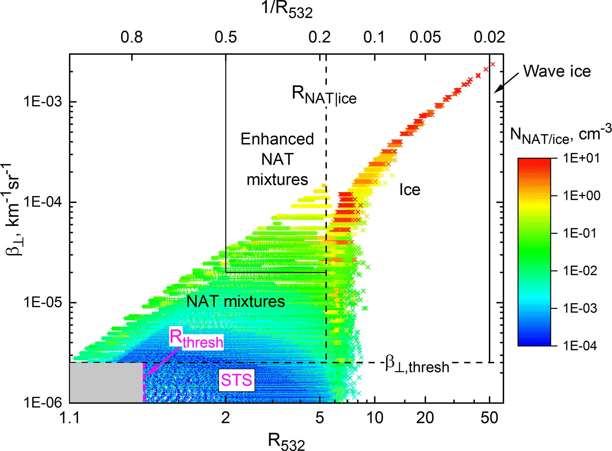
Figure 4Theoretical optical calculations for non-equilibrium liquid–NAT and liquid–ice mixtures, illustrating the v2 PSC composition classification scheme. The grey box at the lower left fall represents points that fall below both CALIOP v2 PSC detection thresholds and are classified as non-features.
Two known deficiencies in the v1 composition classification scheme were pointed out in P13. Due to uncertainty in the CALIOP measurements, the optical space boundaries between PSC composition classes are actually “fuzzy” rather than sharp. Thus, toggling between inferred composition classes over small spatial scales may be due to measurement noise rather than a true change in composition. This is especially true in the case of separating liquid–NAT mixtures into the Mix1, Mix2, and Mix2-enhanced categories. P13 also pointed out that the boundary separating ice and liquid–NAT mixtures must be shifted to larger values of 1∕R532 (smaller values of R532) in the event of denitrification and dehydration to avoid ice PSCs being misclassified as liquid–NAT mixtures (also noted by Zhu et al., 2017). To address these deficiencies, we have significantly improved the composition classification scheme in v2. The improvements are discussed below in the context of Fig. 4, where the theoretical optical results are replotted in the coordinate system β⊥ vs. R532, which are surrogates for the measured attenuated CALIOP quantities and used for PSC detection. As discussed below in Sect. 3.4, the v2 algorithm also incorporates a retrieval of 532 nm particulate backscatter, βparticulate, through which and are later corrected for attenuation due to overlying particulate layers (i.e., the “primes” are removed), allowing for a more robust comparison with the theoretical results. The families of points representing physically possible [NNAT, rNAT] or [Nice, rice] pairs lie at constant β⊥ in Fig. 4, with temperature again decreasing from left to right along each family of points. The following points are to be noted in our revised algorithm:
-
The former Mix1 and Mix2 classes of liquid–NAT mixtures have been combined into a single class named “NAT mixtures” for brevity. (Note that the line and curve separating Mix1 and Mix2 in Fig. 3 disappears with the v2 definition of NAT mixtures.)
-
The former Mix2-enhanced class has been renamed “enhanced NAT mixtures” and it is now defined as the subclass of NAT mixtures with R532>2 and . This conservative boundary was determined empirically by comparing CALIOP Antarctic PSC data to contemporaneous MIPAS observations with and without a belt of NAT clouds formed by heterogeneous nucleation on wave ice PSCs over the Antarctic Peninsula (Höpfner et al., 2006). MIPAS data from 27, 28, and 30 May 2008 (Michael Höpfner, Karlsruhe Institute of Technology, personal communication, December 2017) showed no evidence of these NAT clouds, and only about 2 % of CALIOP NAT mixture data from those days had R532>2 and . In contrast, NAT belt clouds were clearly evident in MIPAS data on 29 May 2008 and 1–2 June 2008, and their locations were matched extremely well by CALIOP NAT mixtures with R532>2 and . In theoretical terms, CALIOP enhanced NAT mixture points correspond roughly to those NAT mixtures with rNAT<3 µm and , which match the MIPAS NAT detection limits (rNAT<3 µm and NAT VD>0.3 µm3 cm−3) reasonably well. Since our criteria defining enhanced NAT mixtures are conservative, the enhanced NAT mixtures subclass is not all-inclusive; i.e., it does not capture all NAT mixture PSCs heterogeneously nucleated in wave ice PSCs.
-
The wave ice class remains the same as in P11, i.e., ice PSCs with R532>50. We reemphasize that this definition of wave ice is not all-inclusive; i.e., some additional ice PSCs are likely associated with mountain waves, but do not meet our stringent wave ice classification criterion.
-
The dashed horizontal line labeled represents qualitatively the CALIOP statistical threshold for detection of PSCs containing non-spherical particles. In practice, this threshold changes with horizontal averaging scale and differs from point to point due to its dependency on u(β⊥). Each data point is assigned a non-spherical particle confidence index CI. Points with CINS>1 are presumed to be PSCs containing non-spherical particles.
-
The dashed magenta vertical line labeled Rthresh represents qualitatively the CALIOP statistical threshold for detection of liquid PSCs. In practice, Rthresh also changes with horizontal averaging scale and differs from point to point due to its dependency on u(R532). Data points classified as STS are those with CINS≤1, but with R532>Rthresh. Each is assigned an STS confidence index CI; CISTS>1.
-
Note that, in practice, there is not a distinct separation between histograms of β⊥ for v2 STS and NAT mixtures. We estimate that 10–15 % of data points in either class may fall in the overlap region and thus could be misclassified.
-
Points in the grey box at the lower left fall below both CALIOP PSC detection thresholds and are classified as non-features. It should be noted that all measured and derived quantities for non-features are also retained in the v2 data product. A comprehensive discussion of so-called “sub-visible” PSCs can be found in the paper by Lambert et al. (2016), who show that they often can be detected through gas-phase uptake of HNO3 as observed by MLS even though they are not detectable as PSCs by CALIOP.
-
The position of the boundary separating NAT mixtures and enhanced NAT mixtures from ice (labeled RNAT|ice) now is calculated dynamically according to the total abundances of HNO3 and H2O vapors. RNAT|ice is based on a parameterization of theoretical calculations of R532 for fully developed STS (assumed to be points between Tice and Tice−1 K) over a wide range of atmospheric pressures and HNO3 and H2O mixing ratios. Total HNO3 and H2O abundances are determined on a daily basis as a function of altitude and DMP equivalent latitude based on nearly coincident “cloud-free” Aura MLS data, where the CALIOP PSC data themselves are used to filter out MLS data affected by uptake in the cloud particles. Then each point with CINS>1 is assigned a NAT|ice confidence index CI. For points classified as ice or wave ice, CINAT|ice>0. For NAT mixtures or enhanced NAT mixtures, CINAT|ice<0.
-
The v2 composition classification extends downward in altitude to the 215 hPa pressure level (∼10 km), the lowest reliable level for Aura MLS HNO3 data that is required to define the location of the NAT-mixture–ice boundary (RNAT|ice) in our classification scheme. All clouds at altitudes below this pressure level are assumed to be ice.
To illustrate that these theoretical calculations resemble actual measurements, composite 2-D histograms of CALIOP PSC data from 10 to 18 July 2008 (which includes the orbital curtain of Fig. 2) are shown in Fig. 5 for the v1 (panel a) and v2 (panel b) coordinate systems. In the interest of examining a quasi-homogeneous ensemble, the data have been restricted to latitudes from 65 to 75∘ S and θ from 475 to 525 K. The most noteworthy feature in Fig. 5a is that the separation between NAT mixtures and ice is not at the fixed value of used in the v1 algorithm, but instead occurs at –0.35. The separation appears to be better captured in Fig. 5b, where the average dynamically calculated RNAT|ice≈2.75 as a result of denitrification and dehydration.
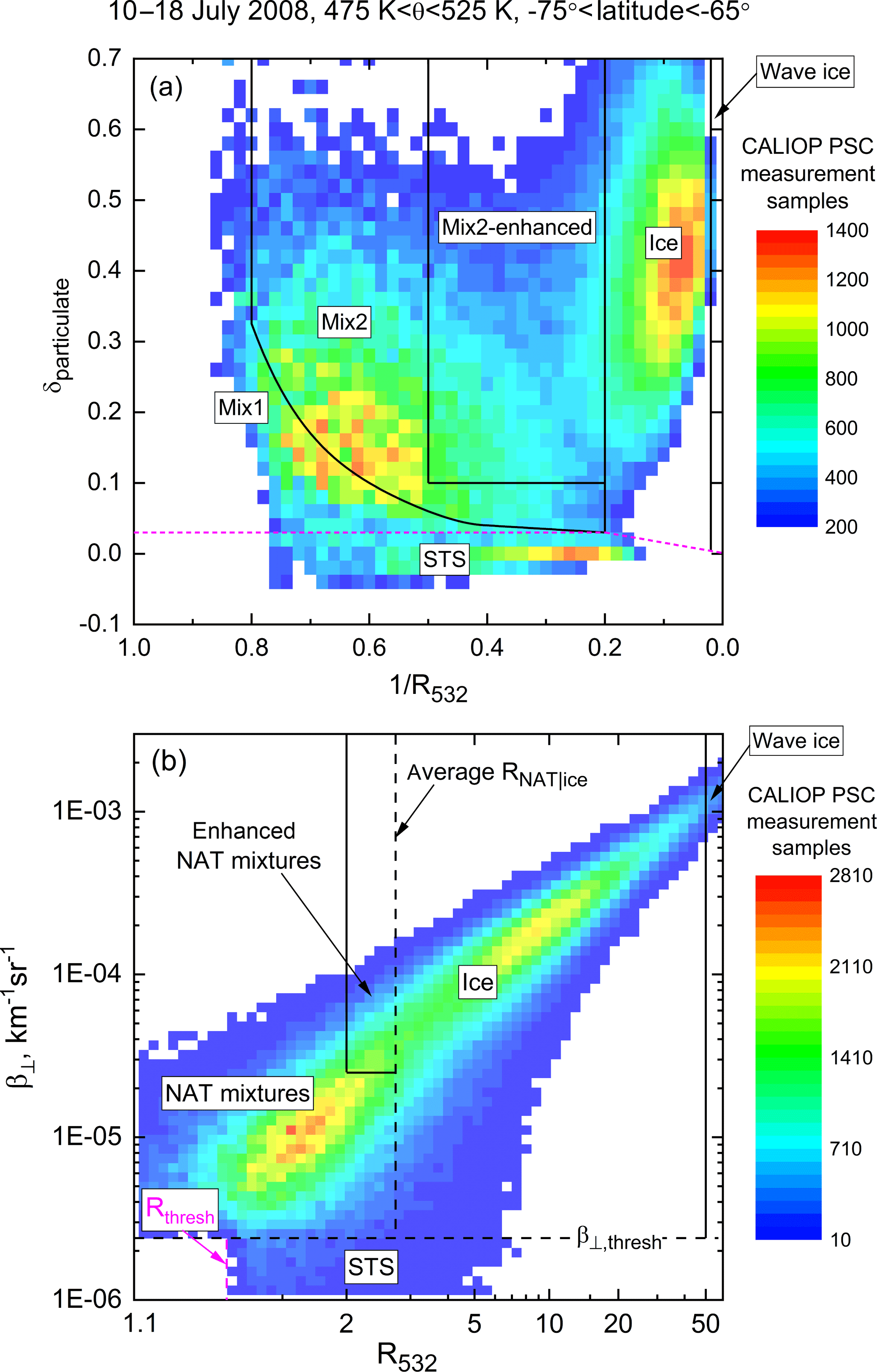
Figure 5The 2-D histogram of CALIOP PSC data for the period 10–18 July 2008, latitudes 65–75∘ S, and potential temperatures (θ) 475–525 K plotted in the CALIOP v1 (a) and v2 (b) composition classification coordinate systems.
3.4 Retrieval of 532 nm particulate backscatter
By retrieving the 532 nm particulate backscatter, βparticulate, the observed quantities and can be corrected for attenuation due to overlying particulate layers (i.e., the primes are removed). This allows for a more robust comparison with the theoretical results and final adjustments in , , and the assigned PSC composition class. It also enables the development of approximate relationships (Sect. 3.5) relating βparticulate to the bulk particle microphysical quantities SAD and VD. The retrieval procedure we have implemented in v2 follows the general CALIOP particulate extinction retrieval approach outlined by Young and Vaughan (2009). The CALIOP total attenuated 532 nm backscatter profile, with the correction for molecular and ozone attenuation previously applied, can be expressed as follows:
where τ(0,z)particulate is the particulate optical depth between the lidar (altitude 0) and altitude z, and η(z) is a factor accounting for multiple scattering. By definition,
where αparticulate(z) is the particulate extinction coefficient.
Making the usual assumption that , where Sparticulate is the particulate extinction-to-backscatter (lidar) ratio, leads to an equation of the form βparticulate(z)=f{βparticulate(z)}, which is solved bin by bin in PSCs layers using an unconstrained top-down Newtonian iterative numerical approach as discussed by Young and Vaughan (2009). The multiple scattering factor η(z) is calculated as a function of temperature from a spline fit to results from Garnier et al. (2015) for semitransparent cirrus clouds; for temperatures <190 K (>240 K) η(z) is fixed at 0.9 (0.5). Based on ground-based 355 nm lidar measurements in a mountain wave PSC event at Esrange, Sweden, Reichardt et al. (2004) derived layer-average values of Sparticulate ranging from 67 to 82 sr (20 to 35 sr) for PSC layers with small (large) scattering ratios. These are consistent with 532 nm Sparticulate values of 50–80 sr derived by Prata et al. (2017) for binary H2SO4–H2O aerosols and with values of 14–26 sr derived by Platt et al. (2011) for cold (−80 ∘C) high-altitude cirrus. For implementation in the v2 algorithm, we derived a parameterization based on the theoretical results described in Sect. 3.3 for binary H2SO4–H2O and STS droplets by which Sparticulate varies smoothly between the observed bounds:
The minimum value of Sparticulate was set at 16 to ensure that retrievals did not terminate at altitudes above where PSCs were detected in the CALIOP level 1 attenuated backscatter data.
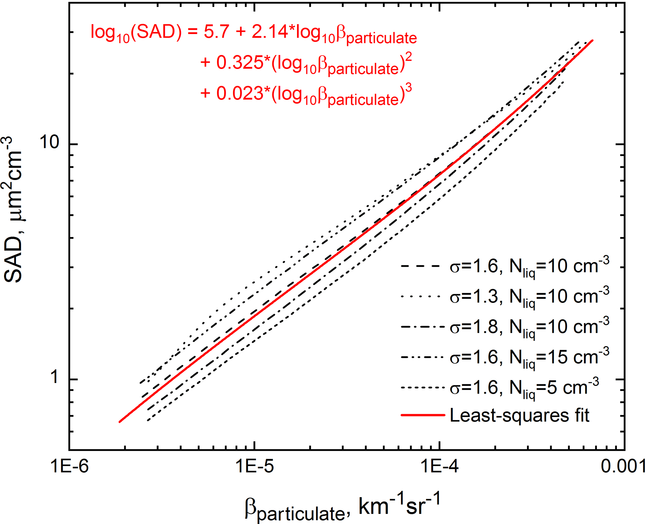
Figure 6Theoretical particulate surface area density (SAD) vs. βparticulate for various combinations of liquid particle number density Nliq and lognormal geometric standard deviation σ, along with the third-order polynomial least-squares fit.
3.5 Estimation of particle SAD and VD
To estimate SAD and VD using CALIOP data, we followed the methodology applied to stratospheric aerosols by Gobbi (1995), in which functional relationships linking βparticulate, SAD, and VD were determined by averaging the scattering properties of a large set of stratospheric aerosol size distributions. Actual PSC particle size measurements are somewhat limited and have often been obtained under mountain wave conditions (e.g., Deshler et al., 2003; Schreiner et al., 2002; Voigt et al., 2003), and there is little or no information on the actual shapes of NAT or ice PSC particles. Therefore, we made the simplifying assumption that useful functional relationships could be based on the averaged scattering properties of a range of size distributions for liquid spherical H2SO4–H2O and STS particles, the characteristics of which are much better constrained. As described in Sect. 3.3, the equilibrium VD for H2SO4–H2O or STS particles can be calculated as a function of temperature for given atmospheric pressure and HNO3 and H2O mixing ratios from Carslaw et al. (1995). Assuming a single-mode lognormal size distribution with number density Nliq and geometric standard deviation σ, the mode radius and SAD can then be calculated from VD using standard relationships between lognormal moments (e.g., Heintzenberg, 1994). With the particle size distribution fully specified, βparticulate can be calculated using the database of optical properties for spherical particles compiled by Scarchilli et al. (2005). To explore the sensitivity of the results to size distribution parameters, we performed calculations for other values of Nliq (5 and 15 cm−3; Wilson et al., 1990; Campbell and Deshler, 2014) and σ (1.3 and 1.8) in addition to our standard conditions of Nliq=10 cm−3, σ=1.6, 50 hPa atmospheric pressure, 10 ppbv HNO3, and 5 ppmv H2O. The results are shown in Figs. 6 and 7, along with the third-order polynomial least-squares fits to the two sets of curves. Note that increases (decreases) in atmospheric pressure, HNO3, or H2O do not produce different curves, but shift the results for a given curve to the right (left). The RSS (root sum of squares) uncertainty in liquid particle SAD due to measurement error and lack of knowledge of the size distribution parameters Nliq and σ is on the order of ±1 (±2.5, ±5) µm2 cm−3 for (10−4, ) . The corresponding RSS uncertainty in liquid particle VD is on the order of ±0.05 (±0.15, ±1.0) µm3 cm−3 for (10−4, ) .
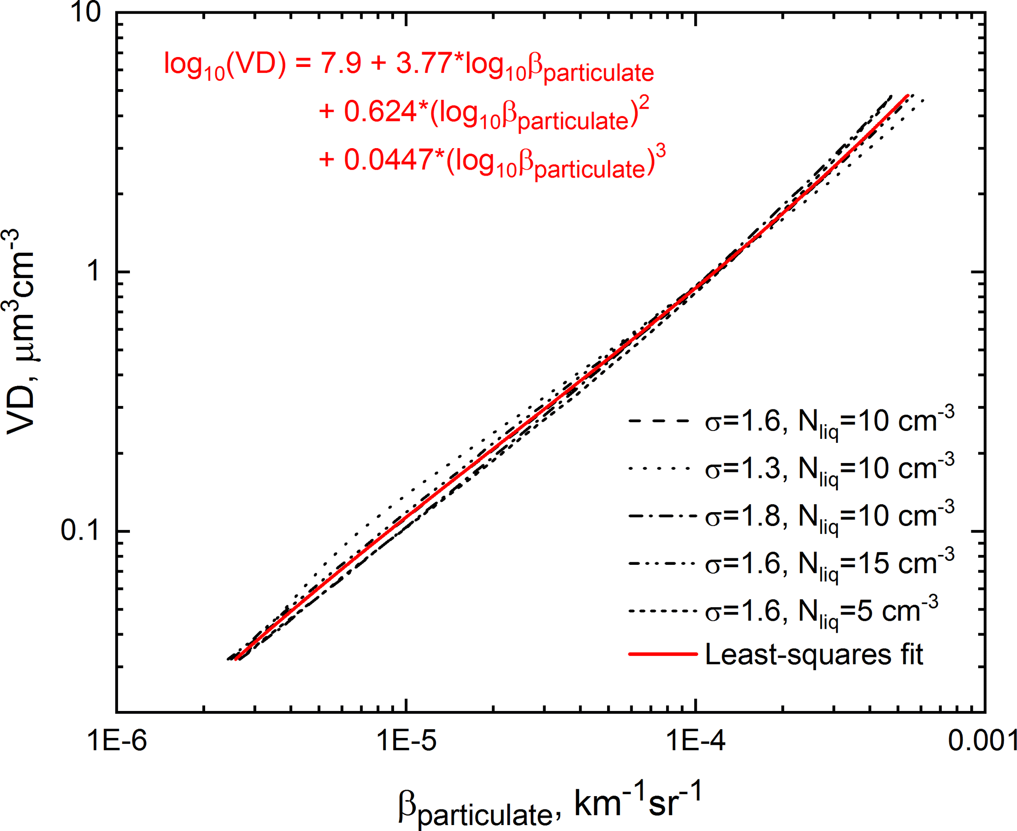
Figure 7Theoretical particulate volume density (VD) vs. βparticulate for various combinations of liquid particle number density Nliq and lognormal geometric standard deviation σ, along with the third-order polynomial least-squares fit.
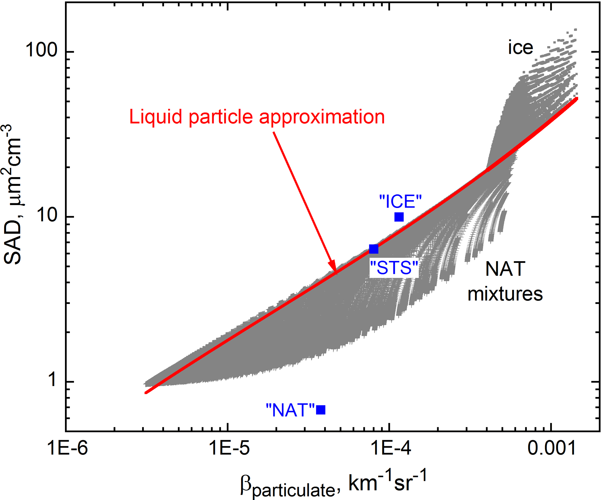
Figure 8Theoretical particulate surface area density (SAD) vs. βparticulate from the full suite of results for NAT mixtures and ice, compared with the liquid particle approximation. Blue symbols are computed values based on bimodal lognormal size distribution fits to in situ optical particle counter measurements within STS, NAT, and ice PSC layers (Deshler et al., 2003).
These liquid particle approximate expressions can be applied to the full suite of CALIOP data, including sub-visible PSCs as well as background aerosols. However, there are large uncertainties in the case of NAT mixtures and ice PSCs due to the dearth of information on NAT or ice particle size and shape. Figures 8 and 9 show the complex behavior of SAD and VD versus βparticulate from the full set of theoretical results for NAT mixtures and ice discussed in Sect. 3.3 and compare those to the liquid particle approximations shown in Figs. 6 and 7. For a given value of βparticulate, the liquid particle approximation for SAD is an upper limit for the actual SAD in NAT mixtures and a lower limit for the actual SAD in ice PSCs. The level of over- or underestimation of SAD may be as much as a factor of 3. For a given value of βparticulate, the liquid particle approximation for VD is a lower limit for the actual VD in ice PSCs and in most NAT mixtures, the exception being those with small rNAT ( µm). The level of underestimation of VD can be as much as a factor of 10 for NAT mixtures and up to a factor of 30 for ice PSCs. To test the validity of our approach, we used bimodal lognormal size distribution fits to in situ optical particle counter measurements within STS, NAT, and ice PSC layers (Deshler et al., 2003) to compute SAD, VD, and βparticulate. These are the blue symbols (labeled according to PSC composition) in Figs. 8 and 9 and show that our estimates of SAD and VD are reasonable.
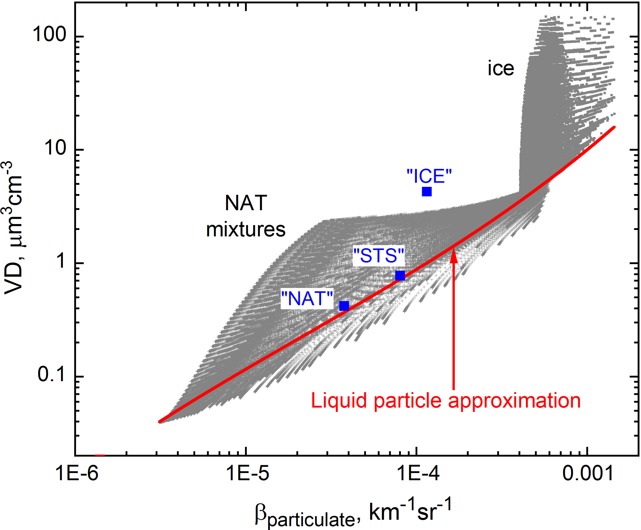
Figure 9Theoretical particulate volume density (VD) vs. βparticulate from the full suite of results for NAT mixtures and ice, compared with the liquid particle approximation. Blue symbols are computed values based on bimodal lognormal size distribution fits to in situ optical particle counter measurements within STS, NAT, and ice PSC layers (Deshler et al., 2003).

Figure 10Curtains of CALIOP (a) R532, (b) β⊥, (c) v2 PSC composition, and (d) v1 PSC composition along the orbit track on 17 July 2008 highlighted in Fig. 1. The location of the MERRA-2 blended tropopause is shown in panels (c) and (d) by the solid black line.
3.6 Illustration of difference between v1 and v2 algorithms
In this section, we illustrate top-level changes in CALIOP PSC data products between the v1 and v2 algorithms. Figure 10a and b present curtains of the retrieved v2 values of the two optical signals used in PSC detection and composition discrimination, R532 and β⊥, for the orbit shown in Fig. 2, and Fig. 10c is the resultant v2 PSC composition curtain. Spatially coherent regions of NAT mixtures/enhanced NAT mixtures (yellow/red) and ice (blue) identified along the orbit track correspond directly to regions of enhancements in both R532 and β⊥, while regions of liquid STS (green) show no enhancements in β⊥ since they are spherical droplets and are identified solely through enhancements in R532 (i.e., near left edge of orbit curtain). Also notice the mountain wave ice (dark blue) with its distinctive tilted layer structure over the Antarctic Peninsula (75∘ S, 300∘ W). For comparison, the v1 PSC composition curtain is shown in Fig. 10d. In general, there is much more ice and much less enhanced NAT mixtures in v2 compared with v1, where much of the ice was misclassified as NAT mixtures due to the fixed boundary separating the two composition classes in v1. In the lower stratosphere–upper troposphere, the v2 composition classification is producing more ice than with v1 due to the improved characterization of the HNO3 and H2O condensables in this region. In addition, v2 substantially fills in holes that are present in the v1 image and reduces the pixel-to-pixel variation in inferred PSC composition. As noted in Sect. 3.3, all clouds at altitudes below the 215 hPa pressure level are assumed to be ice in v2.
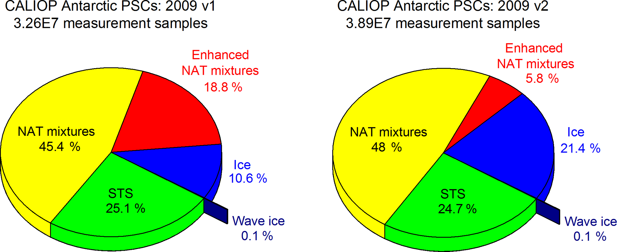
Figure 11Comparison between v1 and v2 CALIOP PSC observations during the 2009 Antarctic winter and their breakdown by composition classification. Data are restricted to altitudes of 4 km or higher above the tropopause to avoid distortion of statistics by ubiquitous underlying cirrus.
Figure 11 compares v1 and v2 in terms of the total number of CALIOP measurement samples within PSCs (180 m vertical by 5 km horizontal pixels) for the Antarctic in 2009 at altitudes of 4 km or higher above the tropopause (to avoid contamination from cirrus), as well as the breakdown of those observations by PSC composition. There are about 19 % more total PSC measurements with v2 due to the less conservative PSC detection thresholds. In terms of PSC composition, the STS, NAT mixture, and wave ice fractions are similar in v1 and v2, but there is a significant decrease in v2 relative to v1 in enhanced NAT mixtures (5.8 versus 18.8 %) and an accompanying increase in ice PSCs (21.4 versus 10.6 %). We estimate that about 75 % of the additional v2 ice PSCs come from a reclassification of v1 Mix2-enhanced PSCs and the remaining 25 % from a reclassification of v1 Mix1 and Mix2 PSCs. Differences between v1 and v2 Antarctic PSC composition for other years and groups of years are comparable to those shown in Fig. 11.
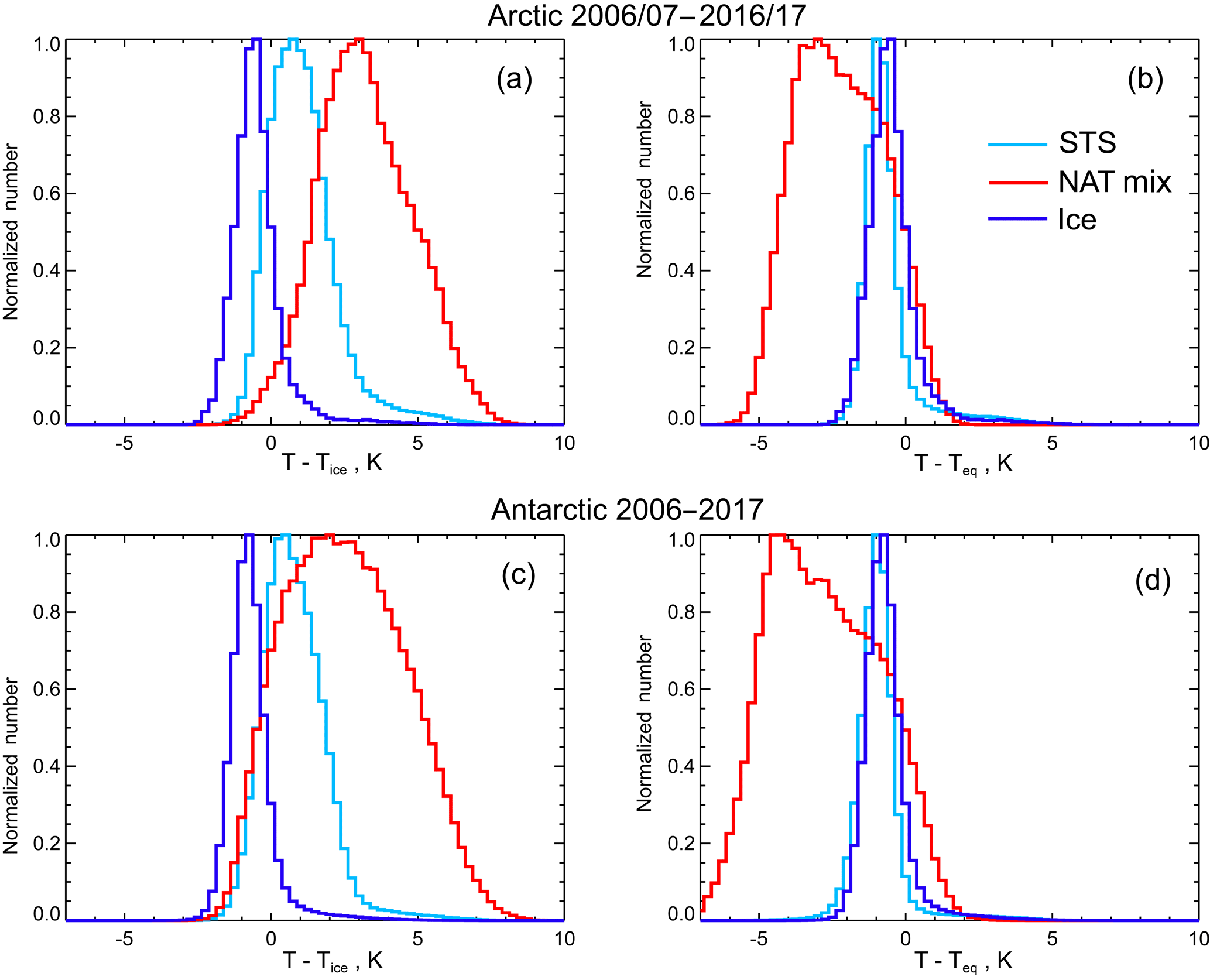
Figure 12Histograms of CALIOP v2 PSC observations at 21 km from 11 Arctic and 12 Antarctic winters as a function of (a, c) T−Tice and (b, d) T−Teq by composition: STS (light blue); NAT mixtures, including enhanced NAT mixtures (red); and ice, including wave ice (dark blue).
3.7 Consistency of v2 PSC observations with expected thermodynamic regimes
Similar to the approach used by Lambert et al. (2012), P13, and Lambert and Santee (2018), we have examined the consistency of the v2 PSC composition classes with respect to their expected thermodynamic existence regimes through combined analyses of the CALIOP and Aura MLS data. Here we extend these previous studies to now include the entire 2006–2017 v2 CALIOP data record. To avoid potentially biased MLS HNO3 measurements where the relatively large geometric field of view (FOV) is only partially filled with PSCs (e.g., see P13 and Lambert and Santee, 2018), the analyses are limited to cases where CALIOP PSCs cover at least 75 % of the Aura MLS FOV (assumed to be 165 km×2.16 km) and a single CALIOP composition is dominant. Composite histograms of PSC occurrence vs. T−Tice over the 20–22 km altitude range are shown in Fig. 12a and c for the Arctic (2006–2007 to 2016–2017) and Antarctic (2006–2017), respectively. Here, T is the ambient temperature at the CALIOP observation point determined from the MERRA-2 gridded analyses, and Tice is calculated using the Murphy and Koop (2005) relationship with the coincident Aura MLS gas-phase H2O abundance. Histograms are shown for the CALIOP STS, NAT mixture (including enhanced NAT mixtures), and ice (including wave ice) composition classes, and each histogram is normalized to a maximum value of 1.0. Figure 12b and d show the same composite histograms transformed to T−Teq space, where Teq is defined as TNAT, TSTS, or Tice, depending on the CALIOP composition classification, and is calculated using the Hanson and Mauersberger (1988) (TNAT), Carslaw et al. (1995) (TSTS), and Murphy and Koop (2005) (Tice) relationships with the coincident HNO3 and H2O abundances observed by MLS. Teq for ice PSCs remains the same as in Fig. 12a and c and the ice PSC distributions are identical to those in Fig. 12a and c. The STS and NAT mixture histograms are restricted to observations with MLS HNO3 values greater than 1 ppbv to avoid the region where the NAT and STS equilibrium HNO3 uptake curves converge (e.g., see Fig. 3 in P13).
The mode of the ice PSC distribution for both hemispheres is located at a temperature slightly below the frost point with a full width at half maximum of about 1 K. The longer positive tail in the ice PSC distributions may be associated with wave ice events induced by small-scale temperature perturbations that are not fully resolved in the MERRA-2 temperature fields (e.g., Hoffmann et al., 2017a) or NAT mixtures at warmer temperatures misclassified as ice due to measurement noise. STS PSCs in both hemispheres occur over a relative narrow temperature range centered slightly below the STS equilibrium temperature. The relatively narrow widths of the ice and STS histograms with modes near Teq are an indication that these particles are near equilibrium, as would be expected. The ice and STS histogram mode peaks occurring below Teq are consistent with a small cold bias in the MERRA-2 temperature analyses as noted by Lambert et al. (2012) and Lambert and Santee (2018). The NAT mixture distributions are broader and roughly bimodal with one mode slightly below the NAT equilibrium temperature and a second more populous mode at 3–4 K below NAT equilibrium, which corresponds approximately to the STS equilibrium temperature. As discussed in P13, this bimodality is likely a consequence of different exposure times of air parcels to temperatures below TNAT. The mode near the STS equilibrium temperature represents air parcels with relatively brief exposure to temperatures below TNAT. These parcels contain non-equilibrium liquid–NAT mixtures with a detectable enhancement in β⊥, but the uptake of HNO3 is dominated by the much more numerous liquid droplets at the lower temperatures. The NAT mixture mode near the NAT equilibrium temperature corresponds to parcels that have been exposed to temperatures below TNAT for extended periods of time, allowing a larger fraction of the gas-phase HNO3 to condense onto the thermodynamically favored NAT particles and bringing the mixture closer to NAT equilibrium. These composite histograms, which incorporate over 11 years of CALIOP PSC measurements, demonstrate behavior consistent with theoretical expectations for each composition class, providing confidence that the v2 composition classification scheme is robust.
Applying the v2 detection and composition classification algorithm to the CALIOP v4.10 lidar level 1B data from June 2006 through October 2017, we have created a new PSC reference data record which covers 12 Antarctic PSC seasons (May–October) and 11 Arctic PSC seasons (December–March). It is archived as the CALIPSO lidar level 2 polar stratospheric cloud mask version 2.0 (v2) data product and publicly available through the NASA Langley Atmospheric Science Data Center (ASDC) (https://eosweb.larc.nasa.gov/project/calipso/lidar_l2_polar_stratospheric_cloud_table, last access: May 2018). In this section, we present representative figures drawn from this data record that depict the seasonal and interannual variability of PSC spatial coverage in the Antarctic and Arctic, climatological mean geographic patterns of PSC occurrence, and overall differences between the hemispheres. We also show how Antarctic PSC composition varies climatologically over the season and relate climatological zonal mean cross sections of PSC occurrence to analogous cross sections of temperature and the PSC condensables HNO3 and H2O. We reiterate that in general we make no explicit attempt to separate upper tropospheric cirrus from PSCs in the climatologies, but do include the location of the MERRA-2 tropopause in many of the figures as a guide to the reader for the approximate upper extent of cirrus. Only in the PSC spatial volume analyses (Figs. 15 and 22) and composition pie charts (Figs. 11 and 25) do we exclude data within 4 km of the tropopause because inclusion of the omnipresent cirrus would skew the statistics on the temporal evolution of PSC occurrence and relative fraction of ice PSCs.
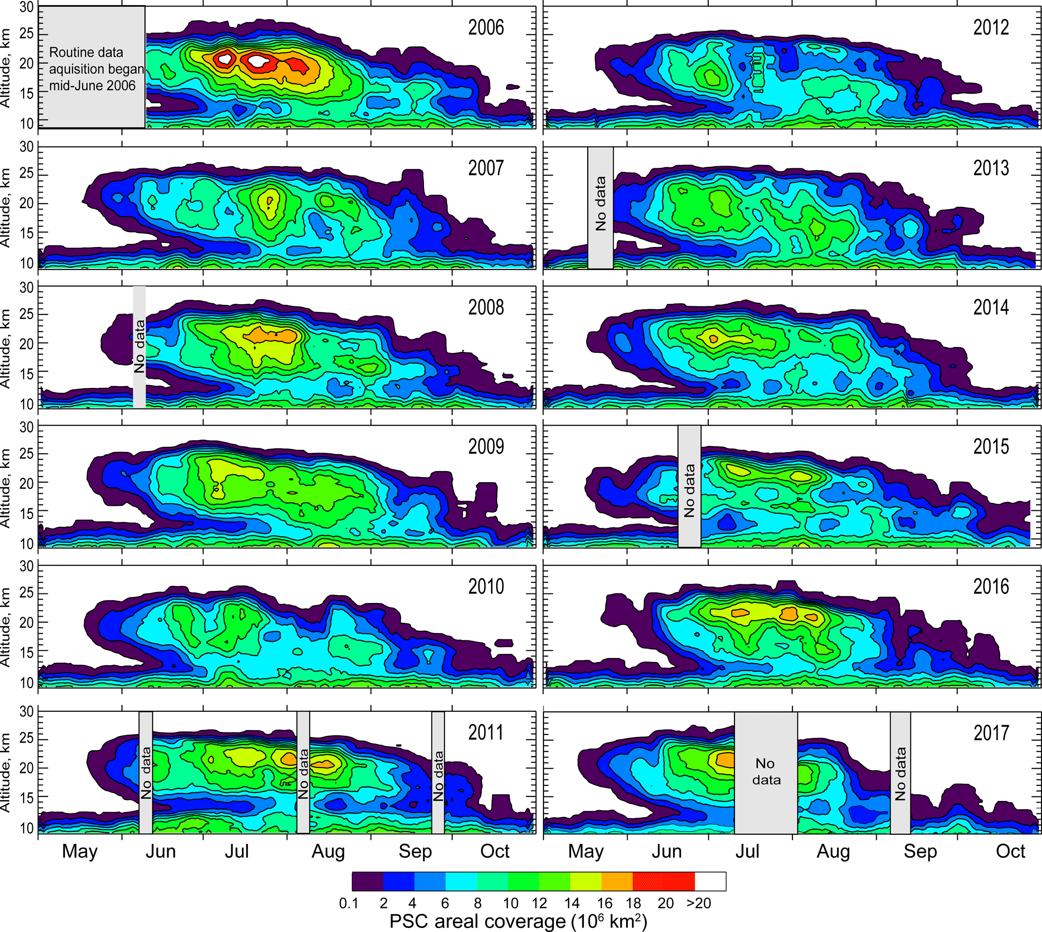
Figure 13Time series of total PSC areal coverage over the Antarctic region as a function of altitude for each of the 12 Antarctic winters in the CALIOP v2 data record.
4.1 Antarctic
4.1.1 PSC areal and spatial volume coverage
A depiction of the vortex-wide, seasonal evolution of PSC occurrence is given by a measure of the total areal coverage of PSCs over the polar region as a function of altitude and time. To mitigate the effects of irregular sampling density due to the CALIPSO orbit geometry, the daily total PSC areal coverage is estimated as the sum of the occurrence frequency (number of PSC detections divided by the total number of observations) in 10 equal-area latitude bands spanning the 50–90∘ S latitude range, multiplied by the area of each band. This estimate implicitly assumes that the CALIOP observations from the approximately 15 orbits per day are representative of the PSC coverage within each latitude band. Note that the highest equal-area latitude band covers 77.8–90∘ S, so CALIOP measurements between 77.8 and 82∘ S are assumed to be representative of the entire 77.8–90∘ S latitude band. A similar approach has been used to estimate PSC area statistics by P09 for CALIOP observations from 2006 to 2008 and also by Spang et al. (2018), who found that MIPAS and CALIOP PSC areas from the 2009 Antarctic PSC season were in excellent agreement in spite of the fundamentally different measurement approaches.
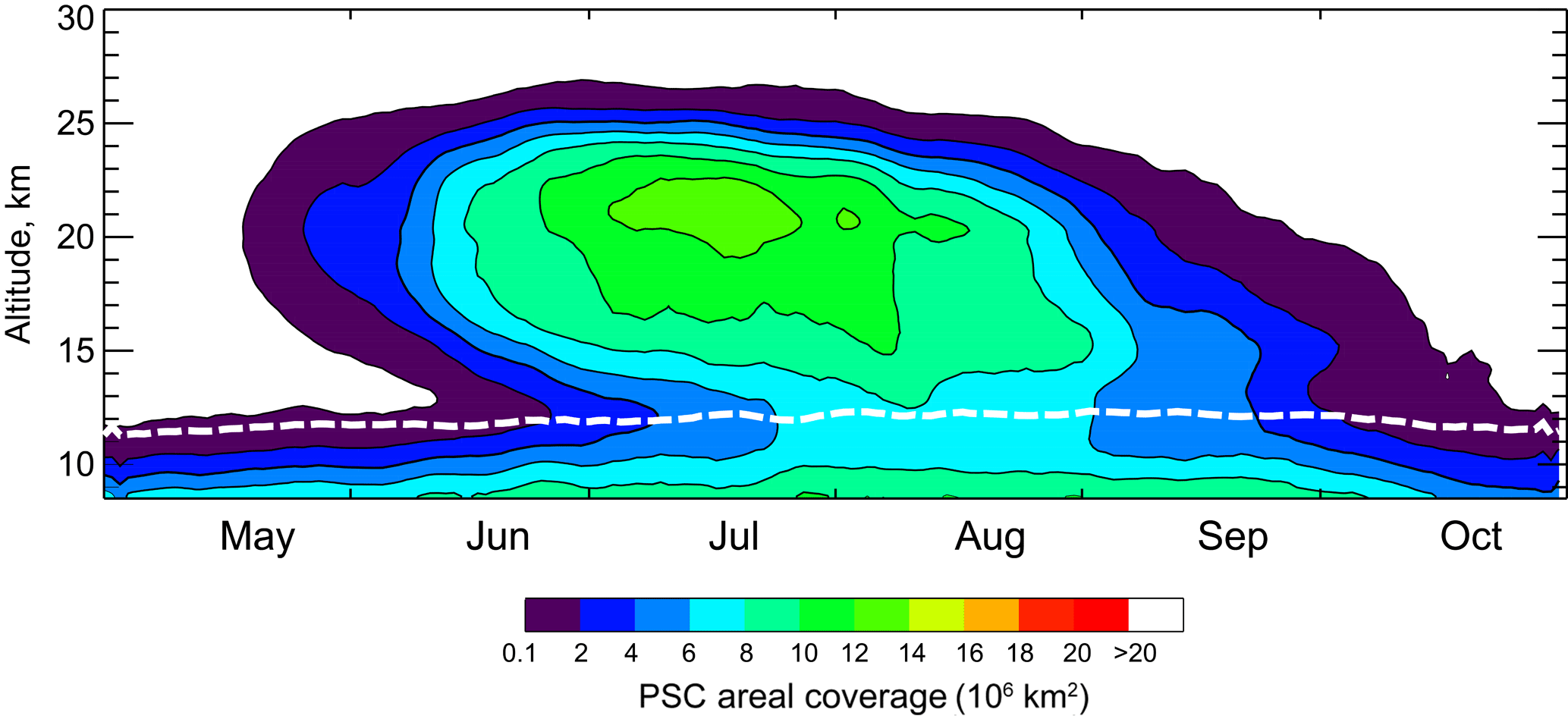
Figure 14Twelve-year mean daily PSC areal coverage over the Antarctic. The climatological daily maximum MERRA-2 tropopause height is indicated by the dashed white line.
The seasonal evolution of PSC areal coverage during each of the 12 seasons in the CALIOP Antarctic data record is shown in Fig. 13. The full altitude range of the PSC data product (8.4–30.0 km) is presented with no attempt here to distinguish PSCs from upper tropospheric cirrus clouds that are commonly observed below ∼12 km throughout the entire season. Temperatures low enough for PSC existence typically occur inside the stratospheric polar vortex, which in the case of the Antarctic is large, relatively axisymmetric, and generally similar from year to year (e.g., Waugh and Randel, 1999). Hence, it is not surprising that the seasonal evolution of PSC coverage in the Antarctic follows a similar pattern from year to year, with PSCs first occurring in mid- to late May and persisting into October. The total areal extent of PSCs typically peaks in July and August when the vortex is largest and coldest and then diminishes markedly in September and approaches zero in October. PSCs extend in altitude from near the tropopause up to >25 km, but there is a downward trend in the altitude of maximum areal coverage over time from above 20 km early in the season to near 15 km by September. This corresponds to a downward shift in the axis of coldest temperatures as the vortex warms at higher altitudes, as was also noted by Poole and Pitts (1994). An interesting feature seen in most years is the apparent merging of the upper tropospheric and lower stratospheric cloud layers in July and August associated with CALIOP observations of deep synoptic-scale clouds extending from the troposphere into the stratosphere to altitudes well above 20 km. These episodic events are likely produced by large-scale adiabatic cooling along upwardly displaced isentropic surfaces above upper tropospheric anticyclones (e.g., Teitelbaum and Sadourny, 1998; Teitelbaum et al., 2001; Kohma and Sato, 2013). Distinctive tilted cloud layers formed in the cold phases of strong orographic gravity waves (e.g., Cariolle et al., 1989; Höpfner et al., 2006; Orr et al., 2015) are also occasionally observed to extend from the troposphere well into the stratosphere, primarily over the Antarctic Peninsula. Both of these phenomena can be seen in the CALIOP orbit curtain shown in Fig. 2.
Although the general seasonal evolution is similar from year to year, there is a moderate amount of year-to-year variability in PSC coverage during the season that is primarily driven by the dynamical processes that control the size, thermal structure, and stability of the vortex, as well as the strength and frequency of orographic and upper tropospheric forcing events. For instance, 2006 was characterized by an especially large and cold vortex (e.g., WMO (World Meteorological Organization), 2007) and showed the largest PSC areas observed by CALIOP to date, while in 2010 and 2012 the vortex was relatively warm with concomitantly much smaller PSC areas. The climatological mean seasonal evolution of Antarctic PSC areal coverage compiled for the 2006–2017 period is shown in Fig. 14. The climatological daily maximum tropopause height is indicated on Fig. 14 by the dashed white line and provides an approximate upper limit to the extent of cirrus during the season. While it is a reasonable approximation to the seasonal evolution of PSC coverage in any given year, the dynamic variability of the vortex, as well as orographic and upper tropospheric forcing, can produce significant deviations from this mean picture. To better quantify the interannual variability in PSC coverage, we calculated the 12-year mean, standard deviation, and range of daily values of PSC spatial volume (daily area coverage integrated over altitude, e.g., see P09). These PSC spatial volumes are shown in Fig. 15, with maximum and minimum values color-coded according to the year in which they occurred. To avoid contamination from the underlying cirrus, the volume calculations include only those CALIOP observations at altitudes more than 4 km above the reported tropopause. Most of the maximum values in PSC spatial volume are from the very cold 2006 season, and many of the minimum values are from the warmer 2010 and 2012 seasons. At the peak of the season in July, the relative standard deviation in PSC spatial volume is about ±25 %.
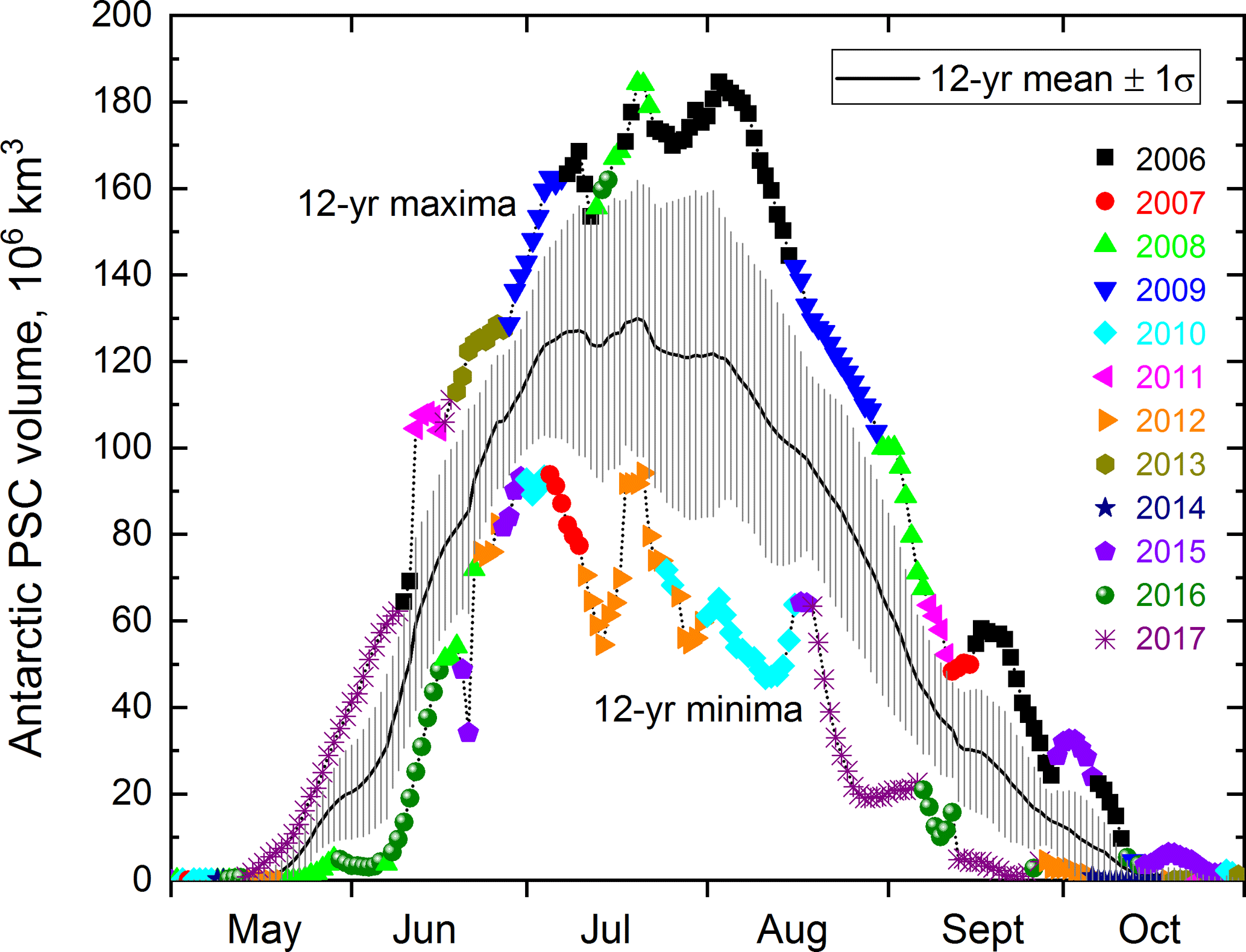
Figure 15Time series of the 12-year mean, standard deviation, and range of daily values of Antarctic PSC spatial volume (daily areal coverage integrated over altitude). The daily maximum and minimum values are color-coded according to the year in which they occurred.
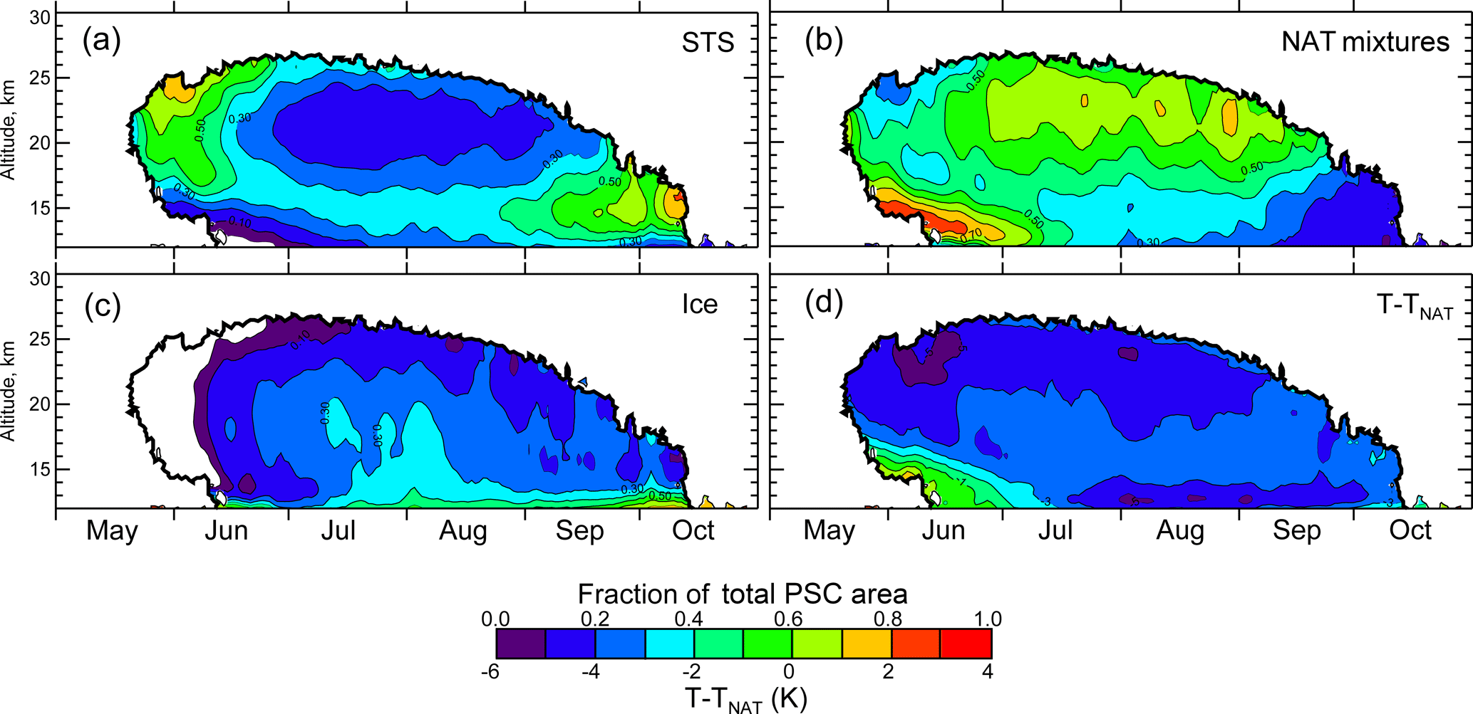
Figure 16Twelve-year mean relative spatial coverage (composition-specific area normalized by total PSC area) for (a) STS; (b) NAT mixtures, including enhanced NAT mixtures; and (c) ice, including wave ice. For additional perspective, (d) shows the 12-year mean distribution of T−TNAT. The thick black contour line on each of the color panels corresponds to the range of days and altitudes where PSCs (of any composition) were observed in at least 6 of the 12 Antarctic seasons.
The v2 CALIOP PSC data record can also be exploited to differentiate the seasonal evolution of PSC areal coverage by composition class. Figure 16 shows the 12-year mean relative spatial coverage (composition-specific area normalized by total PSC area) for (a) STS; (b) NAT mixtures, including enhanced NAT mixtures; and (c) ice, including wave ice. To provide additional perspective, Fig. 16d shows the 12-year mean contour plot of T−TNAT, where again T is the ambient temperature from MERRA-2 gridded analyses and TNAT is calculated using the Hanson and Mauersberger (1988) relationship with cloud-free Aura MLS gas-phase HNO3 and H2O abundances. To put better focus on PSCs, we limit the lower altitude in Fig. 16 to 12 km, near the climatological maximum tropopause as shown in Fig. 14. The onset of the PSC season in the Antarctic depends on the details of the evolving Antarctic polar vortex such as its shape, location, and coldness, which vary significantly from year to year. Lambert et al. (2016) showed that from 2006 to 2015, synoptic-scale HNO3 uptake by PSCs was first observed by Aura MLS as early as 13 May and as late as 28 May. Furthermore, these initial PSCs are often sub-visible and only become detectable by CALIOP some 1–6 days later. Thus, we chose to avoid the highly variable onset period in terms of presenting a representative climatology and restricted our analyses to days and altitudes where PSCs were observed in at least 6 of the 12 Antarctic seasons covered by CALIOP demarcated by the thick black contour line on each of the color panels in Fig. 16. This provides an indication of the climatological temporal and altitude extent of the PSC season. For STS and NAT mixtures (Fig. 16a, b), PSC onset in at least 6 years occurred by approximately 20 May. The onset of ice PSCs (Fig. 16c) is delayed until temperatures drop below the frost point, which is typically mid-June. STS (Fig. 16a) is the most prevalent composition above 20 km until mid-June and then again at lower altitudes in September and October. The early-season predominance of STS above 20 km corresponds to the region of largest temperature departures below TNAT in Fig.16d, which is consistent with an enhanced liquid particle growth regime. The predominance of STS late in the season may be an indication that efficient NAT nuclei have been removed through sedimentation of PSC particles during the winter. NAT mixtures (Fig. 16b) are by far the dominant composition observed below 20 km in May and early June, comprising >80 % of the total observed PSC area below 17 km, and are also the prevailing composition above 20 km during July through mid-September. The early season maximum of NAT mixtures below 17 km corresponds to a region of temperatures near or just below TNAT where liquid particle growth would not be expected. The onset of ice PSCs (Fig. 16c) is delayed 3–4 weeks relative to STS and NAT mixtures, typically occurring around mid-June as temperatures fall below the frost point. The areal extent of ice PSCs is largest in July and August primarily at altitudes below 20 km, but ice is rarely the predominant composition. Note that cirrus contamination is still apparent in the ice distributions (Fig. 16c) above 12 km. The 12-year mean relative PSC composition breakdown shown in Fig. 16 is remarkably similar to the 2006–2008 compilation shown by P09, highlighting the robustness of these results.
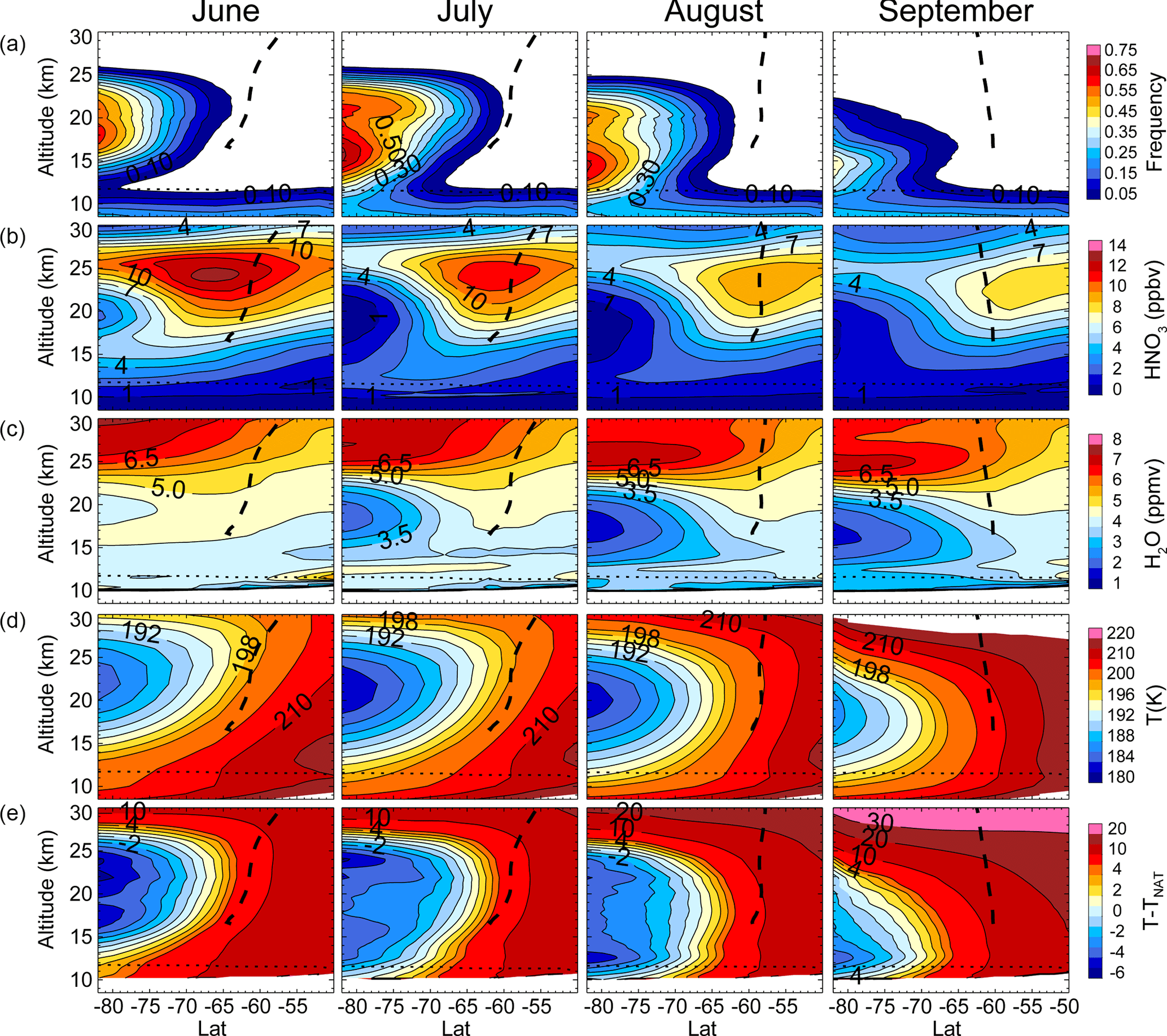
Figure 17Latitude–altitude cross sections of 12-year average, monthly zonal mean (a) Antarctic PSC occurrence frequency, (b) cloud-free MLS HNO3, (c) cloud-free MLS H2O, (d) MERRA-2 temperature, and (e) T−TNAT. For reference, the mean location of the vortex edge (heavy dashed line) and MERRA-2 tropopause height (dotted line) are indicated in the panels.
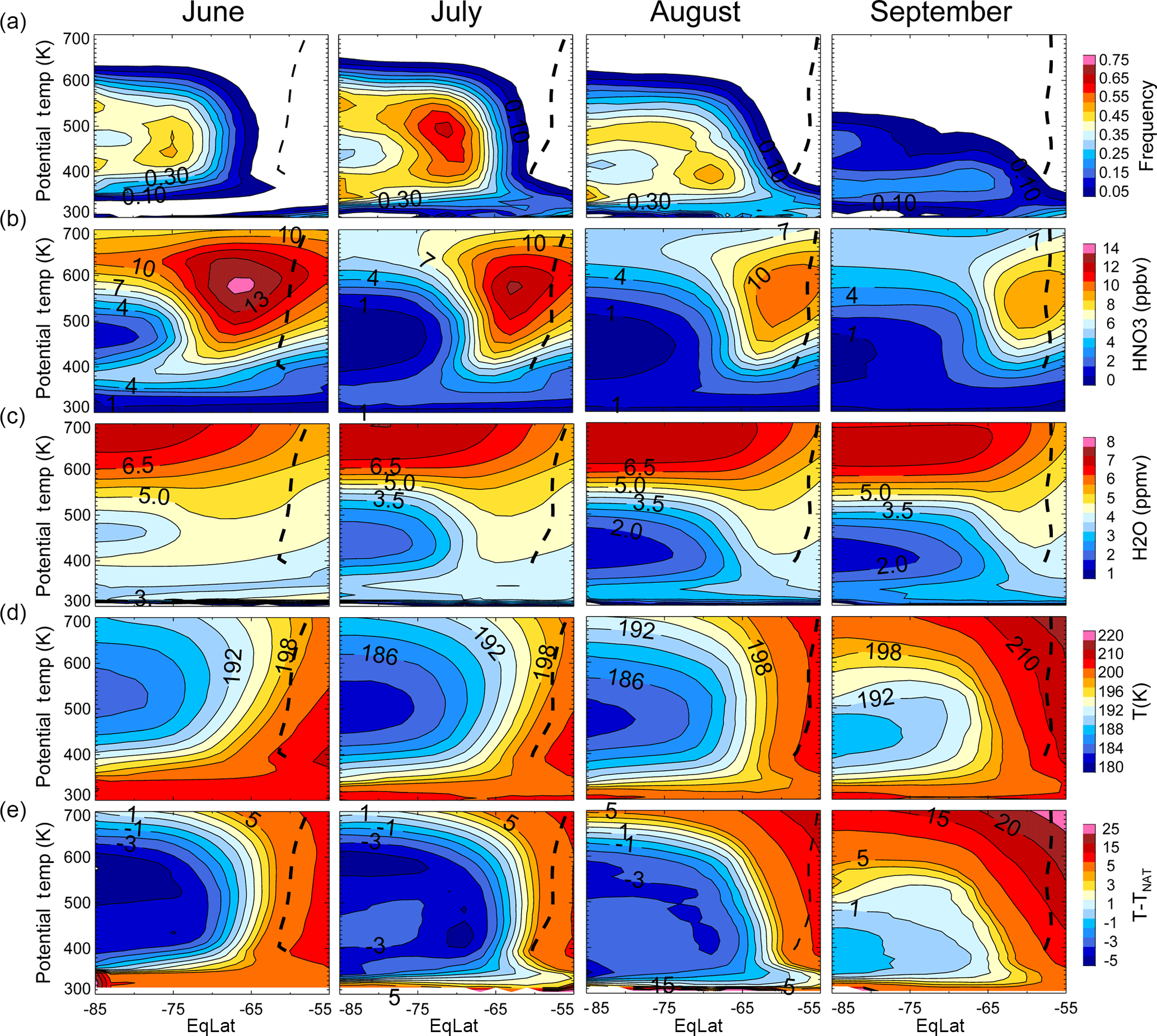
Figure 18Equivalent-latitude–potential-temperature cross sections of 12-year average, monthly zonal mean (a) Antarctic PSC occurrence frequency, (b) cloud-free MLS HNO3, (c) cloud-free MLS H2O, (d) MERRA-2 temperature, and (e) T−TNAT. For reference, the mean location of the vortex edge (heavy dashed line) is indicated in the panels.
4.1.2 Zonal mean and geographical distributions of PSC occurrence
The PSC areal coverage and spatial volume plots capture quite well the seasonal evolution and interannual variability of PSCs from a vortex-wide point of view, but offer no information on the actual geographical patterns of occurrence. To gain this insight, we now examine monthly zonal mean cross sections and polar maps of PSC occurrence frequency. Latitude–altitude cross sections of monthly zonal mean PSC occurrence frequency compiled from the 12-year CALIOP Antarctic data record are shown in Fig. 17 (top row) for the four primary Antarctic PSC months of June–September. To indicate potential PSC existence regimes, we show corresponding cross sections of zonal mean cloud-free MLS HNO3 (second row) and H2O (third row), MERRA-2 T (fourth row), and T−TNAT (bottom row). For reference, the mean location of the edge of the vortex from the Aura MLS DMPs and the tropopause altitude from MERRA-2 are indicated on the panels by the black dashed and dotted lines, respectively. In June, PSCs are observed at latitudes poleward of about 65∘ S from near the tropopause up to about 26 km in altitude, with maximum mean occurrence frequency >60 % near 18 km at the highest latitudes. PSC occurrence peaks during July and August, with the region of highest occurrence frequency expanding in both altitude and latitude in response to the continued cooling of the polar vortex. There is also a hint of a double peak in occurrence frequency with altitude during these months with the dominant peak near 15 km and a secondary peak above 20 km. PSC occurrence declines significantly in both magnitude and spatial extent in September with only a small region of occurrence frequency >40 % at 14 km near 82∘ S and overall occurrence restricted to altitudes below 23 km as the vortex warms at higher altitudes. As was observed in the vortex-wide PSC areal coverage plots, there is a systematic shift downward in the altitude of maximum zonal mean PSC occurrence from near 18–20 km in June to below 15 km in September. Upper tropospheric cirrus cloud occurrence frequency is >10–15 % throughout the season at all latitudes.
Although these conventional latitude–altitude zonal means are correct in a statistical sense, the Eulerian view has the disadvantage of possibly averaging together air masses from different, physically distinct regions of the vortex or even from inside and outside of the vortex. Consequently, the latitude–altitude zonal means are difficult to interpret in the context of meteorological and microphysical processes within the vortex that control PSC occurrence. This is especially true when the vortex is elongated and/or not centered over the South Pole. An alternative approach is to average data in the more physically based quasi-Lagrangian coordinate system of equivalent latitude (EqLat) versus potential temperature (θ). This coordinate system roughly captures the motion of air parcel ensembles and is widely used by the stratospheric chemistry and dynamics community in studies of polar processes (e.g., Butchart and Remsberg, 1986; Manney et al., 1999).
Figure 18 shows the EqLat–θ cross-sectional representations of the 12-year average, monthly zonal mean Antarctic PSC occurrence frequency, cloud-free MLS HNO3 and H2O, MERRA-2 T, and T−TNAT. During most months, the center of the polar vortex is shifted off the pole so that the conventional latitude–altitude cross-sectional monthly means (Fig. 17) blur the sharp gradients in HNO3 and H2O between the interior and “collar” regions (e.g., Wespes et al., 2009) of the vortex that are much more clearly captured in the EqLat–θ cross sections (Fig. 18). Gas-phase HNO3 and H2O are severely depleted by July in the interior of the vortex at ∘ and θ=400–500 K. Although there is relatively cold air present in this region, the lack of condensables sufficiently lowers the particle thermodynamic existence temperatures (e.g., TNAT) to near or below ambient temperatures, limiting PSC existence. Consequently, the highest PSC frequency more typically occurs at equivalent latitudes closer to the vortex edge where there is an optimal combination of sufficient condensables and cold temperatures, which corresponds reasonably well with the minima in the T−TNAT distributions (bottom row of Fig. 18). The reason that a double-peak vertical structure in PSC occurrence appears at high latitudes in July and August in the latitude–altitude cross sections (Fig. 17) is much clearer in the EqLat–θ coordinate system, which shows a relative minimum in PSC occurrence at θ=450 K (∼18 km) corresponding to the layer of depleted condensables.
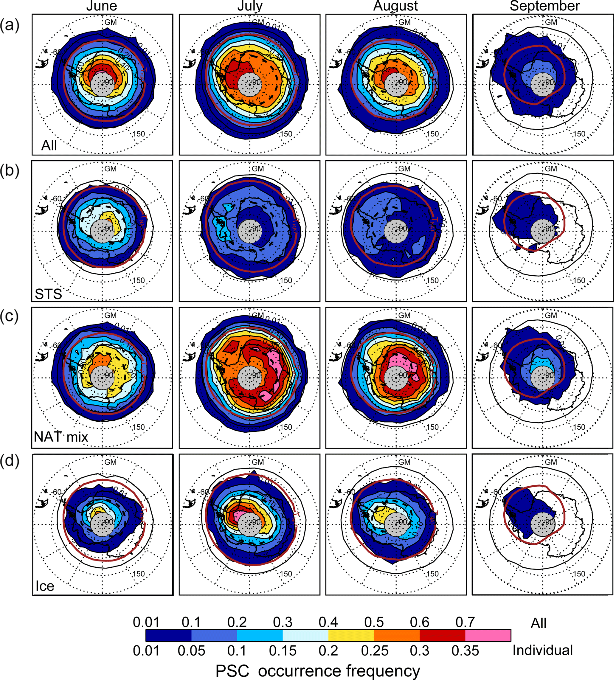
Figure 19Twelve-year average, monthly mean polar maps of Antarctic PSC occurrence frequency at θ=500 K (∼20 km). The top row shows the occurrence frequency for all PSCs, while the subsequent rows display the occurrence frequencies of STS, NAT mixtures (including enhanced NAT), and ice (including wave ice). Overlaid in the panels are the mean location of the edge of the vortex (black line) and the boundaries of the regions where the mean temperature is below TNAT (solid red line) and below Tice (dashed black line). Light gray regions indicate latitudes not sampled by CALIOP. Note the different color scales for “all” PSCs and “individual” compositions.
PSC occurrence is not typically zonally symmetric in either geographic or equivalent latitude coordinate systems, but instead exhibits distinct longitudinal patterns. To illustrate these preferred patterns of PSC occurrence, 12-year average, monthly mean polar maps of Antarctic PSC frequency at θ=500 K (∼20 km altitude) are shown in Fig. 19. The top row shows the occurrence frequency for all PSCs, while the subsequent rows display the occurrence frequencies of STS, NAT mixtures, and ice, respectively. Overlaid in the figure are the mean location of the edge of the vortex (black line) and the boundaries of the regions where the mean temperature is below TNAT (solid red line) and below Tice (dashed black line). In general, PSC occurrence is roughly bounded by the region where mean temperature is below TNAT and increases poleward with the highest occurrence frequencies (>60 %) generally located within the region of T<Tice at the highest latitudes. The contours of PSC occurrence frequency and cold pool are not symmetric around the pole, but are instead pushed slightly off the pole towards the Greenwich Meridian (GM) longitude quadrant. This zonal asymmetry in PSC occurrence is especially pronounced in July–September with the maximum occurrence frequency at 0–90∘ W longitude near the base of the Antarctic Peninsula. The enhancement in PSC occurrence at longitudes near the Antarctic Peninsula is due to frequent mountain wave activity in this region (Alexander et al., 2011, 2013; Hoffmann et al., 2017b) and the large-scale upper tropospheric forcing events which are more frequent at these longitudes (Kohma and Sato, 2013).
The mean geographical distributions of STS, NAT mixtures, and ice PSCs at θ=500 K (Fig. 19, rows 2–4) also exhibit preferred occurrence patterns. STS-only observations are widespread during June at this level, but more limited afterwards with occurrence frequencies generally less than 10 % in the interior of the vortex during July–August and less than 5 % during September. NAT mixtures, on the other hand, are relatively widespread over much of the vortex at this level, especially during July and August when occurrence frequencies exceed 35 %. The ubiquitous NAT mixtures and concomitant limited STS-only observations may be an indication that air parcels well inside the vortex have been exposed to temperatures below TNAT for sufficiently long periods of time to allow the condensed HNO3 to migrate from the STS droplets to the more thermodynamically favored NAT particles. The ring of increased occurrence of NAT mixtures in July over East Antarctica between 70 and 75∘ S latitude is consistent with the so-called NAT belt that evolves downstream of ice PSCs that frequently occur over the Antarctic Peninsula (e.g., Höpfner et al., 2006). Ice PSC occurrence aligns reasonably well with the region of mean temperatures below Tice that occurs over the interior of the vortex at latitudes generally poleward of 70∘ S with a distinct maximum in July and August near the base of the Antarctic Peninsula arising from the frequent mountain wave and upper-tropospheric forcing events in this region.
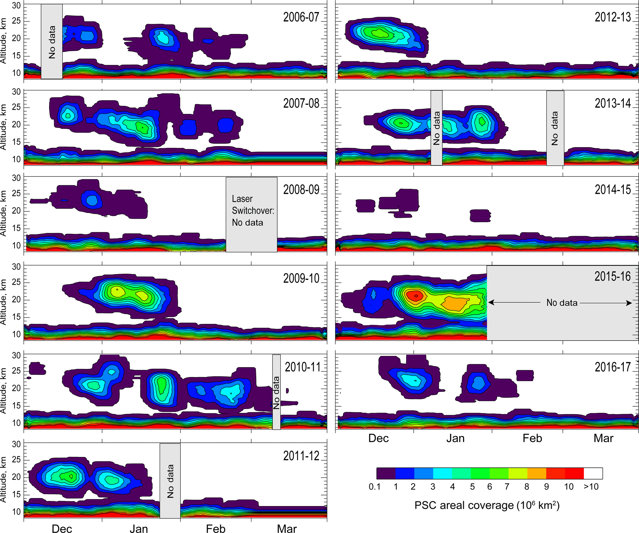
Figure 20Daily PSC areal coverage as a function of altitude for each of the 11 Arctic winters in the CALIOP v2 data record. Note the change in color scale compared with Fig. 13.
4.2 Arctic
4.2.1 PSC areal and spatial volume coverage
The more irregular underlying surface topography in the Northern Hemisphere leads to stronger upward-propagating wave activity than in the Southern Hemisphere, causing a weaker and more distorted Arctic vortex compared to the Antarctic (e.g., Waugh et al., 2017). As a result, the Arctic polar vortex is warmer and exhibits greater temporal variability than its Antarctic counterpart, including sudden stratospheric warmings, which can severely disrupt or even completely break down the vortex in midwinter (Charlton and Polvani, 2007). Not surprisingly then, Arctic PSC occurrence varies significantly from year to year as is illustrated in Fig. 20, which shows the daily mean PSC areal coverage during each of the 11 Arctic seasons in the CALIOP data record. As in Fig. 13, the full altitude range of the PSC data product (8.4–30.0 km) is presented with no attempt here to distinguish PSCs from upper tropospheric cirrus clouds. The 2010–2011 season was marked by persistent periods of PSCs from December to March that set the stage for record ozone depletion over the Arctic (Manney et al., 2011b). During the 2015–2016 season, CALIOP observed the largest areal coverage of PSCs over the Arctic to date, including areas of synoptic ice PSCs, which have only been observed by CALIOP in the Arctic in only one other season (2009–2010). In contrast to these remarkable Arctic PSC seasons, the warm 2014–2015 winter was almost devoid of PSCs. Also note the merging of the upper tropospheric and lower stratospheric cloud layers during some winters (e.g., 2015–2016). As in the Antarctic, this is indicative of upper tropospheric forcing events in the Arctic (Fromm et al., 2003; Achtert et al., 2012) that produce deep synoptic-scale cloud layers extending from the troposphere into the stratosphere.
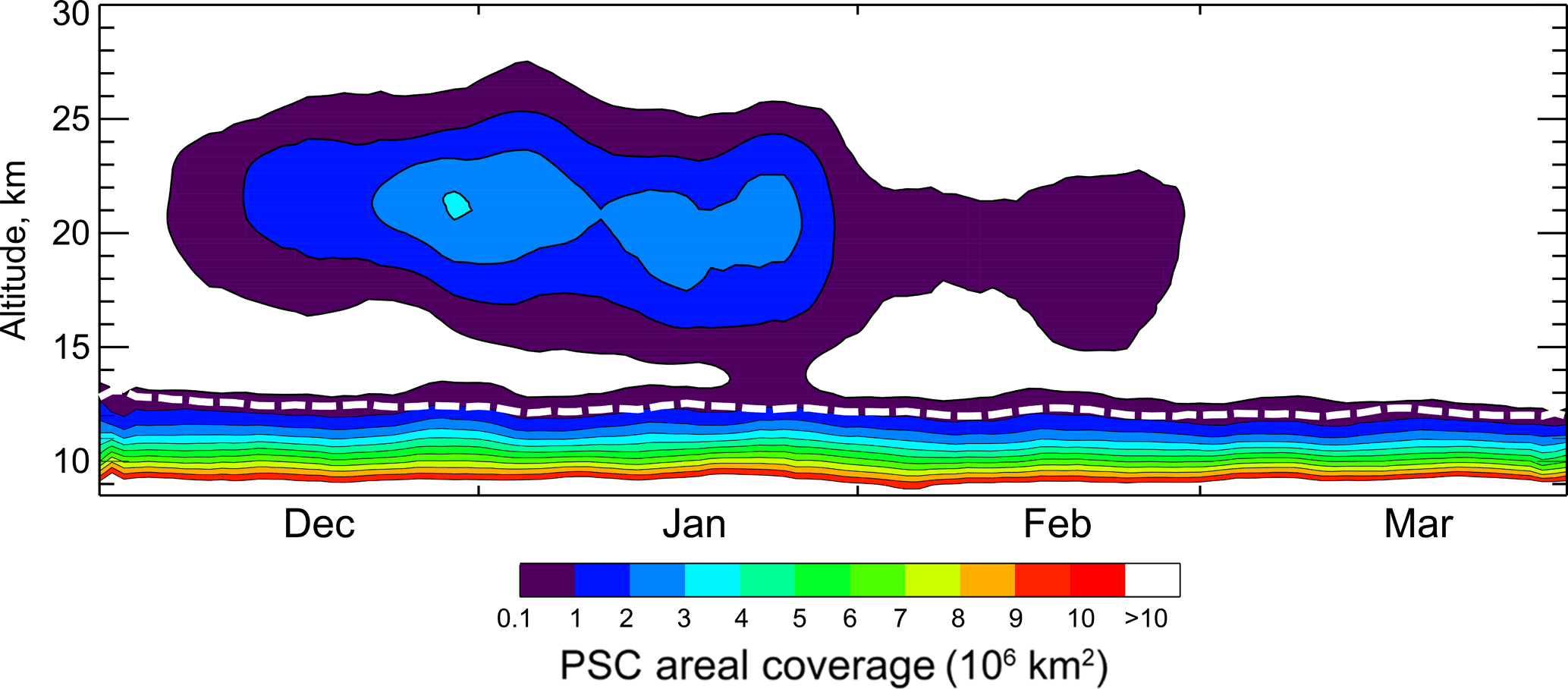
Figure 21Eleven-year mean daily PSC areal coverage over the Arctic. The climatological daily maximum MERRA-2 tropopause height is indicated by the dashed white line.
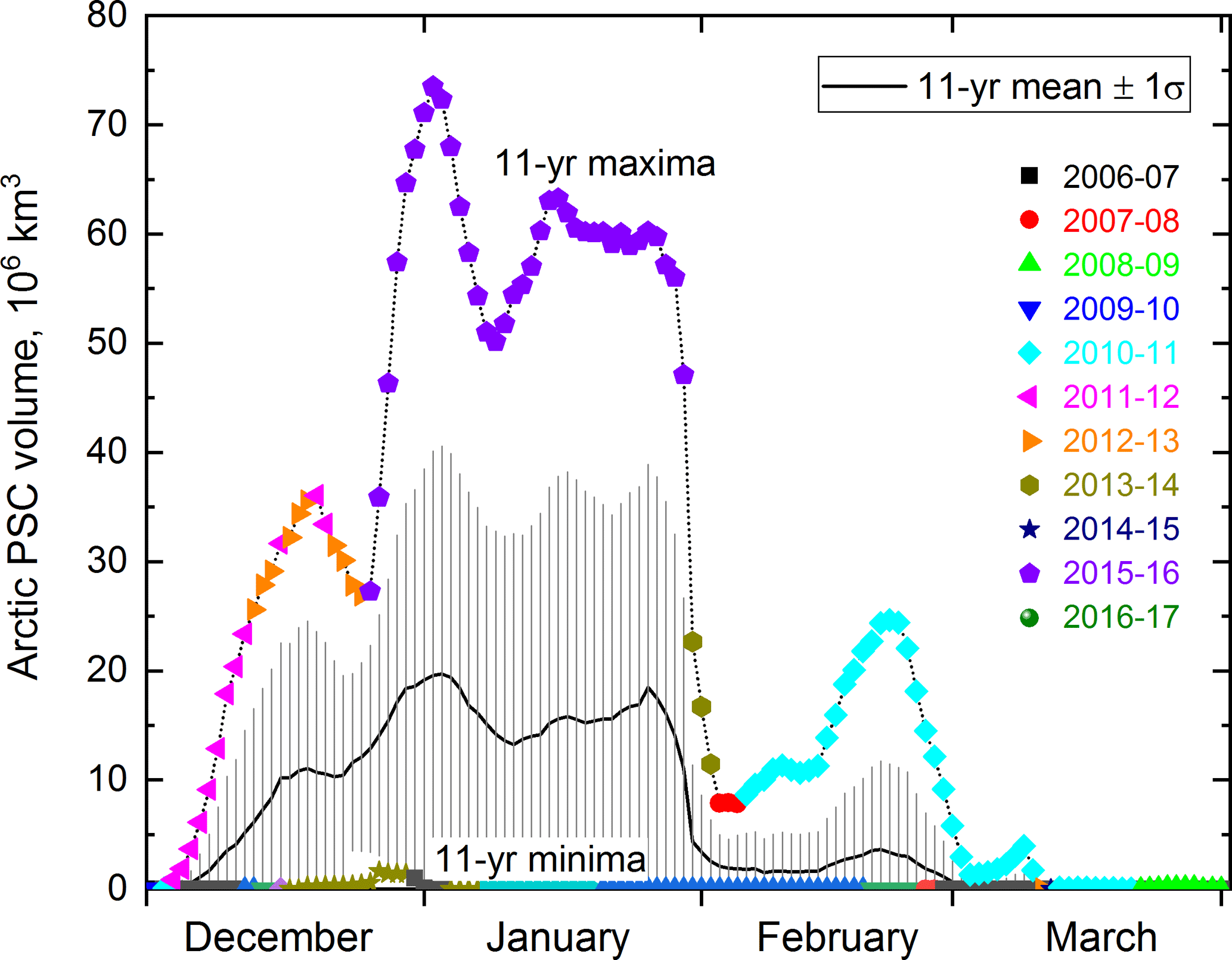
Figure 22Time series of the 11-year mean, standard deviation, and range of daily values of Arctic PSC spatial volume (daily areal coverage integrated over altitude). The daily maximum and minimum values are color-coded according to the year in which they occurred.
For comparison with the Antarctic multi-year mean (Fig. 14), the mean seasonal evolution of Arctic PSC areal coverage compiled for the 2006–2017 period is shown in Fig. 21 with the climatological maximum daily tropopause height indicated by the dashed white line. Clearly the multi-year Arctic mean is unlike any year in the CALIOP record and, hence, would not be very meaningful in itself as guidance for representing Arctic PSCs in a model. The large year-to-year variability in Arctic PSC coverage is further quantified in Fig. 22, which depicts the time series of 11-year mean daily PSC spatial volumes over the Arctic along with the standard deviations, maxima, and minima. All the maxima in January correspond to the anomalous 2015–2016 season while the majority of the maxima in February and March correspond to the 2010–2011 season. The year-to-year variability in the PSC spatial volume in the Arctic is much larger than in the Antarctic, with the relative standard deviations exceeding 100 % for most days. In terms of the climatology of Arctic PSC composition, we feel it is meaningful to show only the composite season-long vertical profile of relative spatial coverage (composition-specific area normalized by total PSC area) in Fig. 23. STS and NAT mixtures are the major Arctic PSC compositions as expected, with STS (NAT mixtures) predominant above (below) 24 km. Note that upper tropospheric cirrus produces the ice maximum near 12 km.
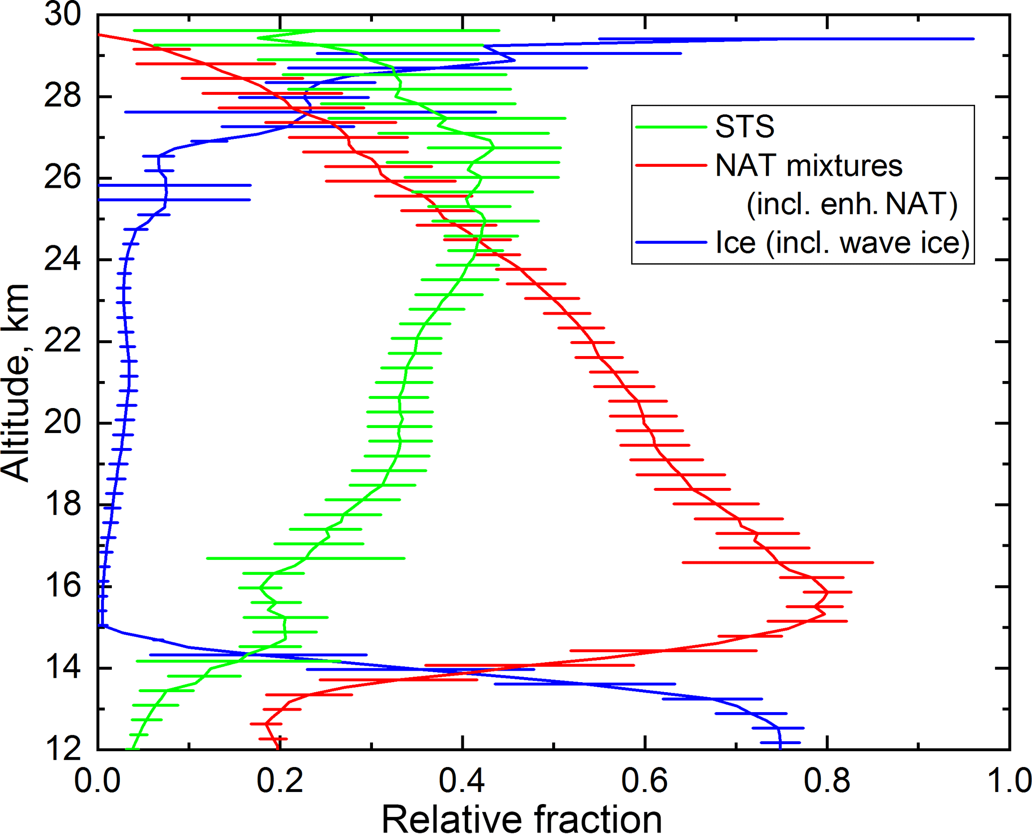
Figure 23Vertical profile of 11-year mean season-long relative spatial coverage (composition-specific area normalized by total PSC area) of Arctic PSCs. Horizontal bars show the standard error in the mean values and are offset by 0.1 km to avoid overlap.
4.2.2 Geographical distributions of PSC occurrence
In spite of the high interannual variability in PSC areal coverage, the geographical pattern of PSC occurrence in the Arctic is quite regular from year to year, with PSCs primarily confined to longitudes from about 60∘ W to 120∘ E as illustrated in the 11-year average, monthly mean Arctic PSC occurrence frequency maps for December and January shown in Fig. 24. This region corresponds to the climatologically favored location of the Arctic vortex in recent decades (e.g., Zhang et al., 2016) which has been influenced by enhanced zonal wavenumber 1 activity, pushing the vortex off the North Pole towards Eurasia.
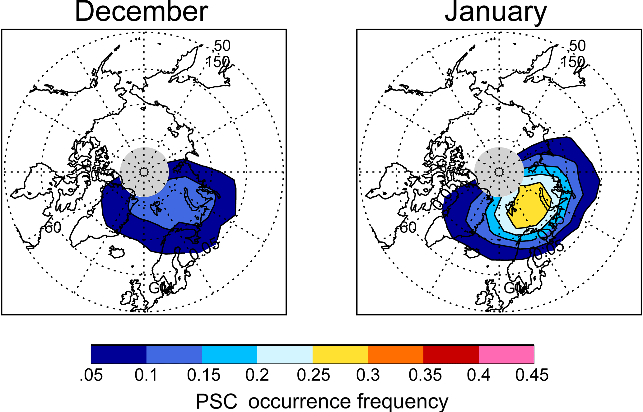
Figure 24Eleven-year average, monthly mean polar maps of Arctic PSC occurrence frequency at θ=500 K (∼20 km). Light gray regions indicate latitudes not sampled by CALIOP.
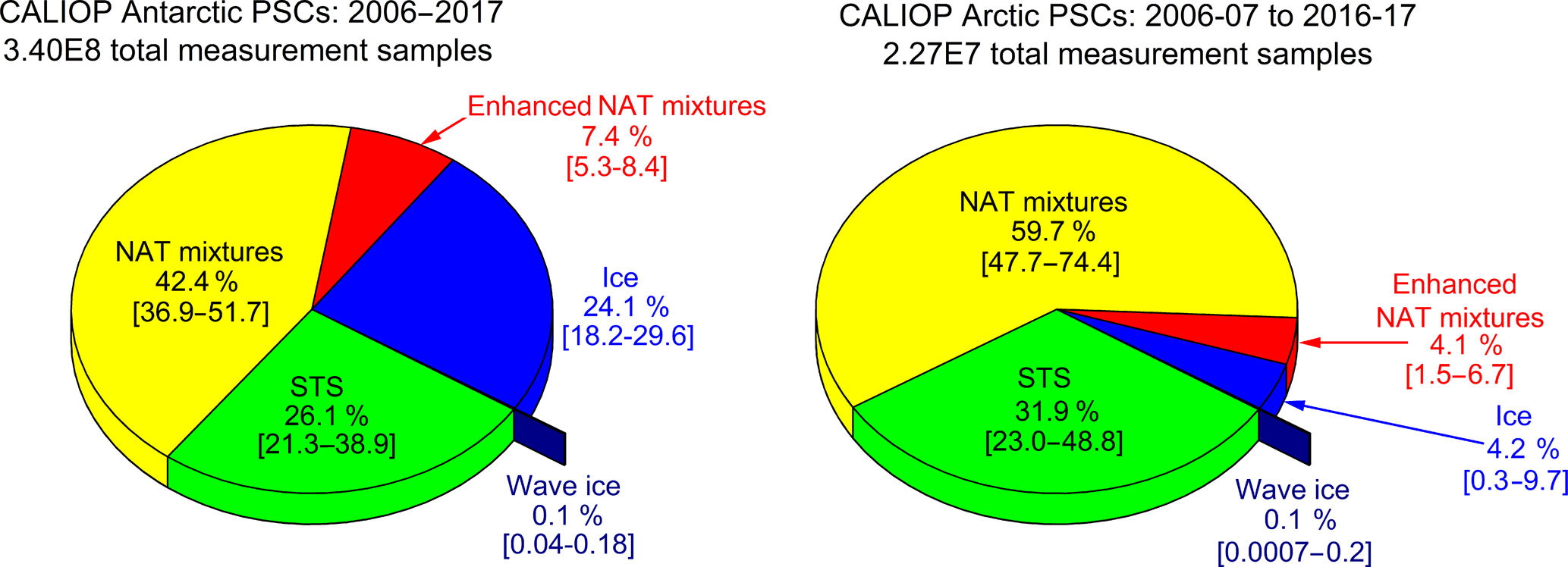
Figure 25Composition breakdown of PSCs observed by CALIOP in the Antarctic and Arctic during 2006–2017. The percentages are averages over the 12 Antarctic and 11 Arctic seasons in the data record, and the minimum and maximum percentages in any one season are indicated by the numbers in brackets. Data are restricted to altitudes of 4 km or higher above the tropopause to avoid distortion of the statistics by ubiquitous underlying cirrus.
4.3 Differences between Antarctic and Arctic
As discussed in Sect. 4.1 and 4.2, the Antarctic polar vortex is a much more conducive environment for PSC existence than its Arctic counterpart. The Antarctic PSC season is longer and more regular with PSCs present every year from mid-May to early October, while in the Arctic PSC occurrence is possible from December to March but not guaranteed in any of these months. The contrast between CALIOP PSC observations in the two hemispheres can be seen in Fig. 25, which shows the total number of measurement samples within PSCs over the entire 2006–2017 data record (12 Antarctic seasons and 11 Arctic seasons), as well as the average, minimum, and maximum percentage of measurements by composition class. On average, about 14 times more PSCs were sampled during a season in the Antarctic than in the Arctic. The largest differences in composition are in ice, which comprised nearly 25 % of Antarctic PSCs compared to less than 5 % in the Arctic (a result of the much colder southern vortex) and in NAT mixtures, which comprised nearly 60 % of Arctic PSCs, but only about 40 % of Antarctic PSCs. The percentages of STS, enhanced NAT mixtures, and wave ice are not vastly different between the two hemispheres.
Figure 26(a) Twelve-year mean seasonal evolution of Antarctic vortex-averaged SAD. (b) Twelve-year average, monthly mean polar maps of SAD over the Antarctic at 18 km for June–September.
As described in Sect. 3.5, estimates of the bulk particle microphysical quantities SAD and VD are included in the new CALIOP v2 PSC data record. The estimates assume liquid particles (binary H2SO4–H2O or STS) only and thus have large uncertainties when NAT mixtures or ice are present. Our estimated SAD is likely an upper (lower) limit for the actual SAD in NAT mixture (ice) PSCs, while our estimated VD is likely a lower limit for the actual VD in ice PSCs and in most NAT mixtures. Nonetheless, they represent the first long-term, vortex-wide observation-based record of SAD and VD and can be used to compare CALIOP stratospheric data with in situ particle measurements and to test parameterizations of the chemical and radiative effects of particles in current and future theoretical models. Since the SAD and VD estimates cover the full range of CALIOP data, including sub-visible PSCs as well as background aerosols, they may prove especially valuable in studies of the role of PSCs relative to that of cold background aerosols in early-season chlorine activation (e.g., Wegner et al., 2016; Drdla and Müller, 2012).
The climatological, 12-year mean depiction of the temporal evolution of vortex-averaged SAD over the Antarctic is shown in the top panel in Fig. 26. The vortex-mean SAD begins to rise in mid-May, which may be an indication of binary aerosol deliquescence as the vortex cools and/or the initial onset of PSCs. SAD increases more significantly in June as PSCs become widespread below 25 km. The maximum SAD and its quasi-periodic nature are associated with ice PSCs that are most prevalent in July and August below 20 km. Twelve-year average, monthly mean polar maps of SAD at 18 km altitude are shown in the bottom row of Fig. 26. Since ice PSCs produce the largest enhancements in SAD, the mean geographical distribution of SAD closely mirrors the highly zonally asymmetric pattern of ice PSC occurrence, with largest values in the 90∘ W to 0∘ longitude sector where ice PSC occurrence is most prevalent, especially in July–September. The spatial and temporal patterns in estimated VD (not shown) are very similar to those in estimated SAD, as expected.
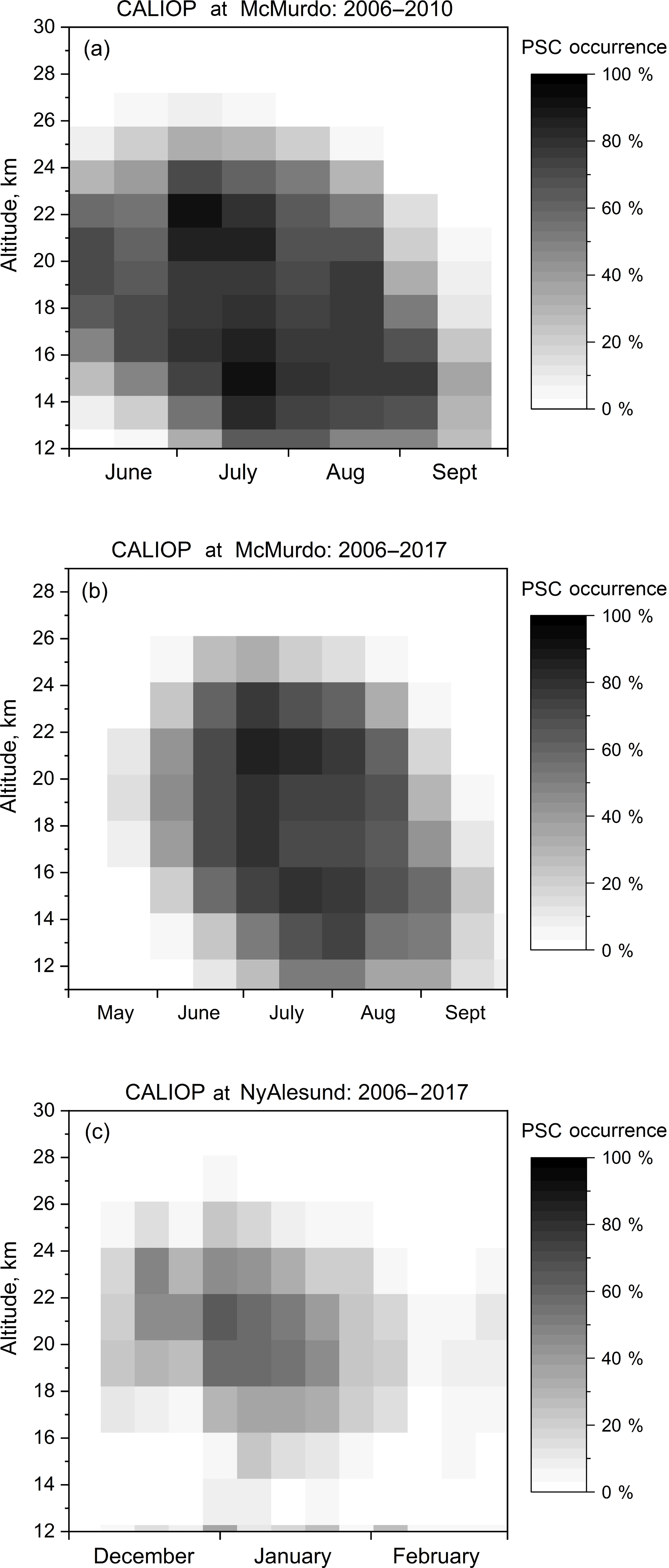
Figure 27CALIOP v2 PSC occurrence frequencies near (a) McMurdo Station, Antarctica, from June to September 2006–2010 (in 15 d×1.5 km bins) for comparison with ground-based lidar data for the same period shown in Di Liberto et al. (2014); (b) McMurdo Station, Antarctica, from May to September 2006–2017 (in 15 d×2 km bins) for comparison with ground-based lidar data from 1995 to 2001 shown in Massoli et al. (2006); and (c) Ny-Ålesund, Spitsbergen, from December to February 2006–2017 (in 7 d×2 km bins) for comparison with ground-based lidar data from 1995 to 2003 shown in Massoli et al. (2006).
In this section we discuss comparisons of CALIOP v2 PSC data with MIPAS PSC observations over the period 2002–2012 and with contemporaneous and historical ground-based lidar PSC observations from McMurdo Station, Antarctica (77.85∘ S, 166.67∘ E), and Ny-Ålesund, Spitsbergen (79∘ N, 12∘ E). Also, to investigate the possibility of longer-term trends, we compare CALIOP PSC data from 2006 to 2017 with the SAM II solar occultation PSC record from the period 1978–1989 (Poole and Pitts, 1994; Fromm et al., 2003).
PSCs are detected and classified in MIPAS data based on differences in IR limb emission spectral measurements from different atmospheric window regions (Spang et al., 2005, 2016). Since this approach is completely different from that of CALIOP, comparisons with MIPAS PSC observations provide an independent test of the validity of the CALIOP PSC results. The first such assessment was presented by Höpfner et al. (2009), who showed a high degree of correlation between MIPAS NAT and CALIOP v1 NAT mixtures for the 2006–2007 Antarctic and the 2006–2007 and 2007–2008 Arctic winters. Spang et al. (2018; hereafter S18) recently published a climatology of PSC occurrence and composition classification based on MIPAS data from 2002 to 2012. S18 compared MIPAS and CALIOP v2 observations of daily, altitude-resolved PSC areal coverage for the 2009 Antarctic season and found excellent correspondence in the overall spatial and temporal evolution as well as for different PSC composition classes. The 10-year mean MIPAS daily PSC areal coverage shown by S18 is very similar to the 11-year mean CALIOP v2 areal coverage (Fig. 14). Additionally, S18 showed the predominant PSC composition to be STS in May and early June and NAT over most altitudes from early July through the end of the season, which is consistent with the CALIOP v2 relative composition areal coverages shown in Fig. 16. In another recent paper, Höpfner et al. (2018) compared retrieved and estimated vertical profiles of PSC particle VD from coincident (within 200 km distance and 2 h time) MIPAS and CALIOP measurements during the 2009 Antarctic winter. For STS PSCs, the comparisons showed very good agreement between the instruments in terms of the vertical profile shape as well as the absolute values of particle VD.
To facilitate comparisons with the ground-based lidar data, we calculated the frequency of CALIOP v2 PSC observations within ±1.5∘ latitude and ±15∘ longitude of McMurdo and Ny-Ålesund, respectively. Figure 27a shows CALIOP PSC occurrence frequencies near McMurdo for June–September 2006–2010 compiled in 15 d×1.5 km bins, which is similar in nature to the ground-based McMurdo 2-D PSC occurrence frequency histogram for the same time period given in Fig. 3 in Di Liberto et al. (2014). Figure 27b extends this to show CALIOP PSC occurrence frequencies near McMurdo for May–September 2006–2017 compiled in 15 d×2 km bins. This figure is quite similar to the 2-D histogram of ground-based lidar PSC occurrence frequencies at McMurdo for the earlier period 1995–2001 shown in Fig. 3b in Massoli et al. (2006). Finally, Fig. 27c shows CALIOP PSC occurrence frequencies near Ny-Ålesund for December–February 2006–2017 compiled in 7 d×2 km bins. This figure is qualitatively similar to the 2-D histogram of Ny-Ålesund ground-based lidar PSC occurrence frequencies for five earlier Arctic seasons from 1995 to 2003 shown in Fig. 3a in Massoli et al. (2006). It is not surprising that the absolute sighting frequencies at Ny-Ålesund by CALIOP and the ground-based lidar do not agree well given the different time periods and the high degree of interannual variability in PSC occurrence in the Arctic (as illustrated earlier in Fig. 22).
The first spaceborne sightings of PSCs were by SAM II (McCormick et al., 1982), which was a single-channel (1 µm) sun photometer (McCormick et al., 1979) that operated on the Nimbus 7 satellite from October 1978 to December 1993 (orbit degradation led to significant data gaps after 1989). SAM II measured the solar radiance in a small (0.01∘) field of view along a tangential ray path through the Earth's atmosphere during each sunrise and sunset encountered by the satellite. The radiance data were reduced to give transmittance profiles, which were then inverted by the methods of Chu and McCormick (1979) to produce 1 km vertical resolution profiles of particulate extinction (αparticulate) at the 1 µm wavelength. Due to the orbital characteristics of Nimbus 7, all sunrise events occurred in the Southern Hemisphere at latitudes from 64 to 81∘ S, and all sunset events occurred in the Northern Hemisphere between 65 and 84∘ N. The measurement locations progressed slowly in latitude (1–2∘ per week) from one extreme to the other over a period of 3 months with the minimum and maximum latitudes measured at the solstices and equinoxes, respectively. There were approximately 14 measurements in each hemisphere per day, each separated by about 26∘ longitude. The SAM II extinction values represent an average over a measurement volume near the tangent point of the optical path, which is approximately 230 km long ×1 km thick. Because of this long horizontal path through the atmosphere, SAM II was very sensitive to the presence of thin cloud that would be transparent to many nadir-viewing instruments. While the inversion treats the atmosphere as a series of concentric shells where the particulate matter in each shell is assumed to be homogeneously distributed throughout the shell, in reality clouds can occur at any point along the ray path at an altitude equal to or higher than the tangent point. With a 12-bit digitizer (Chu and McCormick, 1979), SAM II could not measure through clouds with optical depths greater than about 6 (maximum αparticulate≅0.02 km−1).
The first step in comparing CALIOP with SAM II is to produce a subset of CALIOP data (which we shall call CALIOP-SO) matched to the nominal SAM II solar occultation sampling geometry. For each day from May to November in the Antarctic and from November to March in the Arctic, we determined the longitudes at which the CALIPSO orbits crossed the nominal SAM II measurement latitude(s). We then defined a 230 km along-track ×1 km vertical subset of CALIOP data centered at the SAM II measurement latitude to represent the large occultation sampling volume. If CALIOP detected PSCs in at least five measurement pixels (5 km horizontal ×180 m vertical) within this volume, then the CALIOP-SO measurement was counted as a PSC. The mean CALIOP 532 nm particulate backscatter (βparticulate) in the occultation sampling volume was then calculated. For a given day, we produced 14–15 simulated CALIOP-SO profiles at 1 km vertical resolution from 14 to 30 km in altitude. We repeated this for each day in the CALIOP PSC data record, producing a CALIOP-SO database covering the 2006–2017 period.
For a quantitative comparison of the two datasets, we first converted the CALIOP-SO mean 532 nm βparticulate values to 1 µm αparticulate values using the relationship from Gobbi et al. (1995). We then multiplied the archived SAM II 1 µm αparticulate values by a factor of 1.3 based on the assessment of Thomason et al. (2018), who noted that the SAM II data may be biased low by as much as 30 %. Note that such a bias would have little effect on published SAM II PSC statistics that were based on relative increases in αparticulate. We then produced probability density functions (PDFs) as a function of altitude of calculated 1 µm αparticulate for CALIOP-SO Antarctic PSCs for 2006–2017 and of adjusted (×1.3) SAM II 1 µm αparticulate for Antarctic PSCs detected during the years 1978–1989. We restricted our analysis of the optical signals to the Antarctic because of the large degree of similarity in PSCs there from year to year and omitted the years 1983–1986 from the SAM II composite to avoid the possible masking influence of the 1982 El Chichón eruption. From the PDFs, we determined the season-long minimum (first percentile) detectable values of 1 µm αparticulate for SAM II (×1.3, solid curve) and CALIOP-SO (dotted curve) PSCs, which are plotted as a function of altitude in Fig. 28. These show a clear difference in sensitivity between the instruments, with SAM II able to detect more tenuous PSCs.
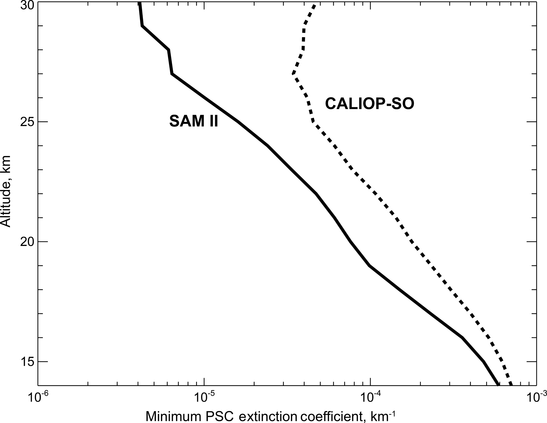
Figure 28Vertical profile of season-long minimum (first percentile) values of adjusted (×1.3) 1 µm αparticulate for SAM II Antarctic PSCs (solid curve) and calculated 1 µm αparticulate for CALIOP-SO Antarctic PSCs (dotted curve).
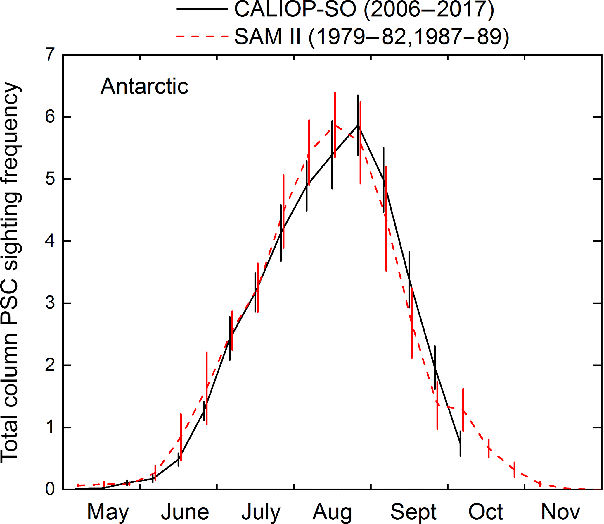
Figure 29Multi-year mean Antarctic PSC column occurrence frequency from May to November for CALIOP-SO (black solid) and SAM II (red dashed), along with standard errors in the means.
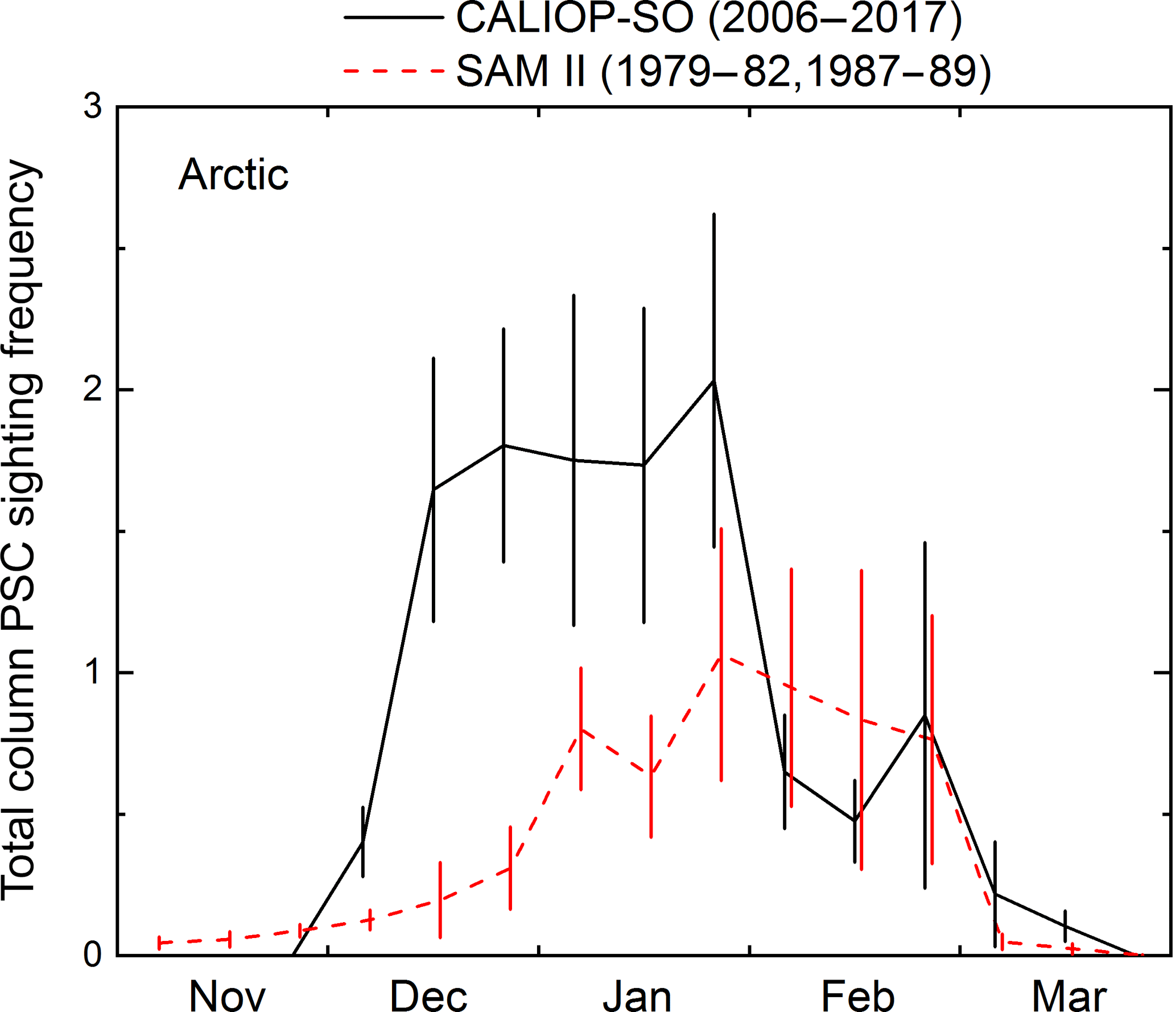
Figure 30Multi-year mean Arctic PSC column occurrence frequency from November to March for CALIOP-SO (black solid) and SAM II (red dashed), along with standard errors in the means.
To put both datasets on equal footing for comparing PSC occurrence frequency, we then reprocessed the SAM II data for PSC detections, excluding all data points with adjusted 1 µm αparticulate that fell below the CALIOP-SO minimum detection threshold. For the CALIOP-SO profiles, we excluded data that would have been beyond the optical depth limit of SAM II, i.e., points with 1 µm αparticulate>0.02 km−1 as well as all points at lower altitudes in those profiles. Figure 29 shows the time series of multi-year mean Antarctic PSC column occurrence frequency for CALIOP-SO (a) and SAM II (b), along with standard errors in the means. Note that the nominal SAM II solar occultation sampling latitude tracks near the terminator, and after September there are no nighttime CALIOP measurements at the SAM II sampling latitude. Overall, the magnitude and variability of the CALIOP and SAM II Antarctic PSC column occurrence frequencies are similar, suggesting there have not been any significant changes since the SAM II era. CALIOP-SO and SAM II column PSC occurrence frequencies for the Arctic are shown in Fig. 30. The two records are similar for February, but the CALIOP-SO occurrence frequencies are significantly higher than SAM II for December and February. This is likely a consequence of the high degree of interannual variability in Arctic PSCs rather than an indicator of a long-term trend.
Measurements from CALIOP on the CALIPSO satellite have greatly expanded the PSC observational data record with now over 11 years of observations to date. The spaceborne lidar profiles the polar stratosphere with unprecedented spatial (5 km horizontal×180 m vertical) and temporal (∼15 orbits day−1) resolution and its dual-polarization capability allows classification of PSCs according to composition. A new v2 CALIOP PSC algorithm has been developed that corrects a number of known deficiencies in previous versions, leading to significantly improved PSC composition data products. Major v2 enhancements include dynamic adjustment of composition boundaries to account for effects of denitrification and dehydration, direct use of measurement uncertainties, addition of composition confidence indices, and retrieval of particulate backscatter, which enables simplified estimates of particulate SAD and VD. Top-level comparisons between v1 and v2 data products indicate that the improved discrimination between ice and NAT mixtures leads to roughly twice as much ice identified in v2 relative to v1, coming primarily at the expense of enhanced NAT mixtures. Composite multi-season histograms of v2 PSC observations in each composition class versus T−Teq were shown to conform to their expected existence regimes, with narrow distributions near Teq for STS and ice, which are thought to be near thermodynamic equilibrium, and a broader bimodal distribution of NAT mixtures due to the frequent non-equilibrium growth of NAT particles. These results are consistent with findings of P13 for the 2006–2009 period, underscoring the robustness of the v2 composition discrimination approach.
Utilizing the v2 algorithm, we have produced a state-of-the-art CALIOP PSC reference data record that spans the June 2006–October 2017 time period with PSC information compiled along each of the ∼15 CALIPSO orbits per day. Nearly coincident Aura MLS measurements of HNO3 and H2O, the primary PSC condensables, along with vortex information from the Aura MLS DMPs have been mapped to the CALIOP PSC along-orbit grid and included in the PSC data products to facilitate their use in the analyses. In combination, this data record represents the most comprehensive, high-resolution PSC database in existence and establishes the foundation for the compilation of a robust climatology of PSC occurrence and particle characteristics. The CALIPSO lidar level 2 polar stratospheric cloud mask version 2.0 (v2) data product is archived at the NASA Langley Science Data Center and available publicly (https://eosweb.larc.nasa.gov/project/calipso/lidar_l2_polar_stratospheric_cloud_table, last access: May 2018).
From the CALIOP PSC reference data record from 2006 to 2017, we have compiled a comprehensive climatology of PSC occurrence and composition for both the Antarctic and Arctic. The seasonal evolution of Antarctic PSC areal coverage corresponds closely to the evolution of the stratospheric polar vortex which is generally similar from year to year in the Antarctic and hence is captured reasonably well by the multi-season mean depiction. However, year-to-year variability in vortex shape, size, and thermal structure leads to moderate variability in PSC coverage, with about 25 % relative standard deviation in PSC spatial volume at the peak of the season in July and August. The relative breakdown of areal coverage by composition shows that STS is the predominant particle composition early in the season above 20 km where temperatures are optimal for liquid particle growth and again late in the season when efficient NAT nuclei may have been depleted. NAT mixtures are predominant in the slightly warmer (T≅TNAT) environment below 16 km in late May and June and also above 17 km from July through mid-September when air parcels have long exposures to T<TNAT, especially in the interior of the vortex, leading to the thermodynamically favored NAT at the expense of STS. Monthly zonal mean cross sections show the multi-season average patterns of PSC occurrence in geographic latitude–altitude and also equivalent-latitude–potential-temperature coordinates. The vortex-centered EqLat–θ coordinates better capture processes controlling PSC existence such as gradients in condensable abundances that are more closely aligned with the structure of the vortex. PSC occurrence is limited deep within the interior of the vortex at high equivalent latitudes due to severe denitrification and dehydration. The maximum in PSC occurrence frequency is typically at EqLats between 65 and 75∘ S, which is closer to the collar region of higher HNO3 near the edge of the vortex.
Geographical patterns of Antarctic PSC occurrence were investigated through examination of polar (latitude–longitude) maps of multi-season, monthly mean PSC occurrence on constant potential temperature surfaces. Overall, there is a maximum in Antarctic PSC occurrence between 90∘ W and 0∘ longitude, which is consistent with the preferential region for forcing by mountain waves and upper-tropospheric anticyclones. CALIOP observations of deep cloud systems that extend from the troposphere well into the stratosphere up to 20–25 km are indicative of the important role of large-scale upper tropospheric forcing in PSC formation. The particle characteristics within these deep cloud systems, particularly in the transition region near the tropopause, are not well understood and warrant further investigation.
Specific compositions also exhibit preferred geographical patterns of occurrence. STS occurrence is typically limited in the interior of the vortex, while NAT mixtures are abundant throughout the vortex. The ubiquitous NAT mixtures and concomitant absence of STS-only observations are likely an indication that air parcels well inside the vortex have been exposed to temperatures below TNAT for sufficiently long periods of time to allow the condensed HNO3 to migrate from STS droplets to the more thermodynamically favored NAT particles. A NAT mixture belt is also seen in the multi-year means over East Antarctica, which is consistent with MIPAS observations (Höpfner et al., 2006). The mean pattern of ice PSC occurrence is dominated by mountain wave forcing, with a maximum in the 90∘ W to 0∘ longitude quadrant near the Antarctic Peninsula.
In contrast to the Antarctic, Arctic PSC occurrence is highly variable from year to year due to the more disturbed Arctic vortex that is prone to sudden stratospheric warmings. As such, the evolution of an Arctic PSC season does not follow a climatological mean pattern and instead each PSC season is distinctly different. For instance, PSC areas during the 2010–2011 and 2015–2016 Arctic seasons were the highest observed during the CALIOP lifetime to date, while the 2014–2015 season was almost devoid of PSCs. As a result, the relative standard deviation in Arctic PSC spatial volume is greater than 100 % throughout most of the season. In spite of the high variability in Arctic PSC occurrence, when PSCs occur they are typically found between 60∘ W and 90∘ E longitude, which is consistent with the preferential location of the Arctic vortex during the last decade. The larger, colder, and more stable Antarctic vortex is much more conducive for PSC formation than the Arctic vortex, leading to about a factor of 14 more PSC observations on average in the Antarctic than Arctic during the CALIOP era. The most compelling difference between the hemispheres in observed composition is in ice, which comprises 24 % of PSC observations in the Antarctic on average, but only 4 % in the Arctic due to the inherently warmer conditions.
Estimates of the bulk particle microphysical quantities SAD and VD are included in the new CALIOP v2 PSC data record. The estimates assume liquid particles (binary H2SO4–H2O or STS) only and thus have large uncertainties when NAT mixtures or ice are present. Our estimated SAD is likely an upper (lower) limit for the actual SAD in NAT mixture (ice) PSCs, while our estimated VD is likely a lower limit for the actual VD in ice PSCs and in most NAT mixtures. Nonetheless, they represent the first long-term, vortex-wide observation-based record of SAD and VD and can be used to compare CALIOP stratospheric data with in situ particle measurements and to test parameterizations of the chemical and radiative effects of particles in current and future theoretical models. A climatology of the seasonal evolution of vortex-averaged SAD was presented, showing an initial increase in May associated with particle growth as the vortex cools, possibly from deliquescence of binary aerosol, and then a more substantial increase as PSCs become widespread in June. Maximum SAD occurs in July and August below 20 km when ice PSCs are most prevalent. Multi-season average, monthly mean polar maps of SAD exhibit a zonally asymmetric pattern that mimics ice PSC occurrence, with maxima occurring near the mountainous Antarctic Peninsula where orography leads to enhanced ice cloud formation.
Comparisons of CALIOP v2 and MIPAS data showed excellent agreement in the overall spatial and temporal evolution of Antarctic PSCs as well as that for different PSC composition classes. CALIOP v2 PSC occurrence frequency patterns in the vicinity of ground-based lidars at McMurdo Station, Antarctica, and Ny-Ålesund, Spitsbergen, are similar in nature to the climatological patterns derived from the ground-based measurements. Finally, to investigate potential longer-term trends in PSC occurrence, appropriately subsampled and averaged CALIOP v2 PSC observations from 2006 to 2017 were compared with PSC data from the 1979–1989 period collected by the spaceborne solar occultation instrument SAM II. The two instruments showed similar magnitude and variability in Antarctic PSC column occurrence frequency, suggesting that there has been no long-term trend. For the Arctic, the two instruments showed similar results for February, but CALIOP column occurrence frequencies were substantially higher than SAM II for December and January. This finding is likely a reflection of the high degree of interannual variability in Arctic PSCs rather than an indicator of a long-term trend.
The data used in this study are available in the following.
-
CALIPSO/CALIOP L1B: Winker (2015).
-
CALIPSO/CALIOP L2 PSC mask: CALIPSO Science Team (2015).
-
Aura MLS HNO3 data: EOS MLS Science Team (2017a).
-
Aura MLS H2O data: EOS MLS Science Team (2017b).
-
Aura MLS derived meteorological products: Manney et al. (2007, 2011a).
-
SAM II Aerosol Extinction data: SAM II Science Team (1999).
A1 Crosstalk correction
The CALIOP backscatter signal is separated into parallel (∥) and perpendicular (⊥) components by a polarization beam splitter in the receiver subsystem (Hunt et al., 2009). With an ideal beam splitter, the measured molecular depolarization ratio (δmol,meas) would equal the theoretical value of 0.00366 at the ∼40 pm bandwidth of the etalon in the CALIOP receiver (Cairo et al., 1999; Hostetler et al., 2006). The difference between the measured and theoretical molecular depolarization ratios indicates the level of crosstalk (CT) between the two polarization channels. We assume for simplicity that a fraction CT of the received parallel signal is reflected into the perpendicular channel and that the remainder (1−CT) of the received parallel signal is transmitted into the parallel detector. With this assumption and some algebraic manipulation, it can be shown that
The crosstalk-corrected attenuated backscatter signals can then be derived from the measured signals as follows:
Figure A1 shows a time series of CT calculated from daily values of δmol,meas over the course of the CALIPSO mission, as well as the PSC season averages used for simplicity in our algorithm. The abrupt jumps in CT are all associated with events in which the etalon temperature was changed, suggesting that they are real changes due to hysteresis associated with temperature cycling of the etalon and its mount. CT has been less than 0.5 % over the entire mission except for the 2008 Antarctic and 2008–2009 Arctic winters, when it was 0.6–0.65 %. δmol has not been measured regularly since March 2015, so a constant value of CT has been assumed after that point.
Figure A1Time series of CT calculated from daily values of δmol,meas over the course of the CALIPSO mission, as well as the averages over PSC seasons.
A2 Random measurement uncertainties
Random uncertainties in [] and [] due to shot noise are computed using the noise-scale factor approach introduced by Liu et al. (2006) and described in detail for the CALIOP system by Hostetler et al. (2006). The uncertainties are scaled by the inverse square root of the product of the number of 15 m vertical bins being averaged, which is 12 in the case of our fixed 180 m vertical resolution; and the number of 1/3 km horizontal resolution laser shots being averaged, which ranges from 15 to 405 in our successive horizontal averaging scheme. Relative random uncertainty in attenuated scattering ratio [] is calculated as the square root of the sum of squares of the relative random uncertainties in [] and [] plus an assumed 3 % relative uncertainty in βmol (Hostetler et al., 2006). The basic random uncertainties are propagated through the calculation of other optical quantities to estimate their uncertainties as well.
MCP and LRP developed the CALIOP v2 PSC algorithm. LRP performed the theoretical optical calculations used for CALIOP v2 PSC composition classification. MCP processed the CALIOP, MLS, MERRA-2, and Aura MLS DMP data. RG performed the initial processing of the SAM II data and SAM-II–CALIOP comparisons. MCP and LRP wrote the manuscript and produced the figures with contributions from RG.
The authors declare that they have no conflict of interest.
The authors would like to thank David Considine, Program Scientist for the
CALIPSO and CloudSat missions, for continued support of this research. The
authors also acknowledge the Stratosphere-troposphere Processes And their
Role in Climate (SPARC) project and the International Space Science
Institute (ISSI) for its support of the SPARC Polar Stratospheric Cloud
Initiative (PSCi). Support for Lamont R. Poole is provided under NASA contract
NNL16AA05C. Michael C. Pitts and Lamont R. Poole would like to pay special tribute to our late
colleague William H. (Bill) Hunt, a senior lidar engineer who made many
significant contributions to the success of atmospheric lidar programs at
NASA Langley over his 40-year career. A testament to his thoroughness and
dedication is the fact that CALIOP has exceeded its expected lifetime many
times over.
Edited by: Rolf Müller
Reviewed by: four anonymous referees
Achtert, P. and Tesche, M.: Assessing lidar-based classification schemes for polar stratospheric clouds based on 16 years of measurements at Esrange, Sweden, J. Geophys. Res., 119, 1386–1405, https://doi.org/10.1002/2013JD020355, 2014.
Achtert, P., Karlsson Andersson, M., Khosrawi, F., and Gumbel, J.: On the linkage between tropospheric and Polar Stratospheric clouds in the Arctic as observed by space–borne lidar, Atmos. Chem. Phys., 12, 3791–3798, https://doi.org/10.5194/acp-12-3791-2012, 2012.
Alexander, S. P., Klekociuk, A. R., Pitts, M. C., McDonald, A. J., and Arevalo-Torres, A.: The effect of orographic gravity waves on Antarctic polar stratospheric cloud occurrence and composition, J. Geophys. Res.-Atmos., 116, D06109, https://doi.org/10.1029/2010JD015184, 2011.
Alexander, S. P., Klekociuk, A. R., McDonald, A. J., and Pitts, M. C.: Quantifying the role of orographic gravity waves on polar stratospheric cloud occurrence in the Antarctic and the Arctic, J. Geophys. Res.-Atmos., 118, 11493–11507, https://doi.org/10.1002/2013JD020122, 2013.
Bosilovich, M. G., Lucchesi, R., and Suarez, M.: MERRA-2: File Specification, GMAO Office Note No. 9 (Version 1.1), 73 p., available at: https://gmao.gsfc.nasa.gov/GMAO_products/reanalysis_products.php (last access: July 2018), 2016.
Butchart, N. and Remsberg, E.: The area of the stratospheric polar vortex as a diagnostic for tracer transport on an isentropic surface, J. Atmos. Sci., 43, 1319–1339, https://doi.org/10.1175/1520-0469(1986)043<1319:TAOTSP>2.0.CO;2, 1986.
Cairo, F., Di Donfrancesco, G., Adriani, A., Pulvirenti, L., and Fierli, F.: Comparison of various linear depolarization parameters measured by lidar, Appl. Optics, 38, 4425–4432, https://doi.org/10.1364/AO.38.004425, 1999.
CALIPSO Science Team: CALIPSO/CALIOP Level 2, Polar Stratospheric Cloud Data, version 1.00, Hampton, VA, USA, NASA Atmospheric Science Data Center (ASDC), https://doi.org/10.5067/CALIOP/CALIPSO/CAL_LID_L2_ PSCMask-Prov-V1-00_L2-001.00 (last access: October 2017), 2015.
Campbell, P. and Deshler, T.: Condensation nuclei measurements in the midlatitude (1982–2012) and Antarctic (1986–2010) stratosphere between 20 and 35 km, J. Geophys. Res.-Atmos., 119, 137–152, https://doi.org/10.1002/2013JD019710, 2014.
Cariolle, D., Muller, S., Cayla, F., and McCormick, M. P.: Mountain waves, polar stratospheric clouds, and the ozone depletion over Antarctica, J. Geophys. Res., 94, 11233–11240, https://doi.org/10.1029/JD094iD09p11233, 1989.
Carslaw, K. S., Luo, B. P., and Peter, T.: An analytic expression for the composition of aqueous HNO3-H2SO4 stratospheric aerosols including gas phase removal of HNO3, Geophys. Res. Lett., 22, 1877–1880, https://doi.org/10.1029/95GL01668, 1995.
Charlton, A. J. and Polvani, L. M.: A new look at stratospheric sudden warmings. Part I: Climatology and modeling benchmarks, J. Climate, 20, 449–469, https://doi.org/10.1175/JCLI3996.1, 2007.
Chu, W. P. and McCormick, M. P.: Inversion of stratospheric aerosol and gaseous constituents from spacecraft solar extinction data in the 0.38–1.0 µm range, Appl. Optics, 18, 1404–1413, 1979.
Crutzen, P. J., Müller, R., Brühl, C., and Peter, T.: On the potential importance of the gas phase reaction and the heterogeneous reaction in “ozone hole” chemistry, Geophys. Res. Lett., 19, 1113–1116, https://doi.org/10.1029/92GL01172, 1992.
Deshler, T., Larsen, N., Weissner, C., Schreiner, J., Mauersberger, K., Cairo, F., Adriani A., Di Donfrancesco, G., Ovarlez, J., Ovarlez, H., Blum, U., Fricke, F., and Dörnbrack, A.: Large nitric acid particles at the top of an Arctic stratospheric cloud, J. Geophys. Res., 108, 4517, https://doi.org/10.1029/2003JD003479, 2003.
Di Liberto, L., Cairo, F., Fierli, F., Di Donfrancesco, G., Viterbini, M., Deshler, T., and Snels, M.: Observation of polar stratospheric clouds over McMurdo (77.85∘ S, 166.67∘ E) (2006–2010), J. Geophys. Res.-Atmos., 119, 5528–5541, https://doi.org/10.1002/2013JD019892, 2014.
Drdla, K. and Müller, R.: Temperature thresholds for chlorine activation and ozone loss in the polar stratosphere, Ann. Geophys., 30, 1055–1073, https://doi.org/10.5194/angeo-30-1055-2012, 2012.
Engel, I., Luo, B. P., Pitts, M. C., Poole, L. R., Hoyle, C. R., Grooß, J.-U., Dörnbrack, A., and Peter, T.: Heterogeneous formation of polar stratospheric clouds – Part 2: Nucleation of ice on synoptic scales, Atmos. Chem. Phys., 13, 10769–10785, https://doi.org/10.5194/acp-13-10769-2013, 2013.
EOS MLS Science Team: MLS/Aura Near-Real-Time L2 Nitric Acid (HNO3) Mixing Ratio V004, Greenbelt, MD, USA, Goddard Earth Sciences Data and Information Services Center (GES DISC), https://disc.gsfc.nasa.gov/datacollection/ML2HNO3_NRT_004.html, last access: October 2017a.
EOS MLS Science Team: MLS/Aura Near-Real-Time L2 Water Vapor (H2O) Mixing Ratio V004, Greenbelt, MD, USA, Goddard Earth Sciences Data and Information Services Center (GES DISC), https://disc.gsfc.nasa.gov/datacollection/ML2H2O_NRT_004.html, last access October 2017b.
Fahey, D. W., Gao, R. S., Carslaw, K. S., Kettleborough, J., Popp, P. J., Northway, M. J., Holecek, J. C., Ciciora, S. C., McLaughlin, R. J., Baumgardner, D. G., Gandrud, B., Wennberg, P. O., Dhaniyala, S., McKinney, K., Peter, T., Salawitch, R. J., Bui, T. P., Elkins, J. W., Webster, C. R., Atlas, E. L., Jost, H., Wilson, J. C., Herman, R. L., and Kleinbohl, A.: The detection of large HNO3-containing particles in the winter Arctic stratosphere, Science, 291, 1026–1031, 2001.
Fromm, M., Alfred, J., and Pitts, M.: A unified, long-term, high-latitude stratospheric aerosol and cloud database using SAM II, SAGE II, and POAM II/III data: Algorithm description, database definition, and climatology, J. Geophys. Res., 108, 4366, https://doi.org/10.1029/2002JD002772, 2003.
Garnier, A., Pelon, J., Vaughan, M. A., Winker, D. M., Trepte, C. R., and Dubuisson, P.: Lidar multiple scattering factors inferred from CALIPSO lidar and IIR retrievals of semi-transparent cirrus cloud optical depths over oceans, Atmos. Meas. Tech., 8, 2759–2774, https://doi.org/10.5194/amt-8-2759-2015, 2015.
Gelaro, R., McCarty, W., Suárez, M. J., Todling, R., Molod, A., Takacs, L., and Zhao, B.: The Modern-Era Retrospective Analysis for Research and Applications, version 2 (MERRA-2), J. Climate, 30, 5419–5454, https://doi.org/10.1175/JCLI-D-16-0758.1, 2017.
Gobbi, G. P.: Lidar estimation of stratospheric aerosol properties: Surface, volume, and extinction to backscatter ratio, J. Geophys. Res., 100, 11219–11235, https://doi.org/10.1029/94JD03106, 1995.
Hanson, D. R. and Mauersberger, K.: Laboratory studies of the nitric acid trihydrate: Implications for the south polar stratosphere, Geophys. Res. Lett., 15, 855–858, https://doi.org/10.1029/GL015i008p00855, 1988.
Heintzenberg, J.: Properties of the Log-Normal Particle Size Distribution, Aerosol Sci. Technol., 21, 46–48, https://doi.org/10.1080/02786829408959695, 1994.
Highwood, E. J., Hoskins, B. J., and Berrisford, P.: Properties of the arctic tropopause, Q. J. Roy. Meteorol. Soc., 126, 1515–1532, https://doi.org/10.1002/qj.49712656515, 2000.
Hoffmann, L., Hertzog, A., Rößler, T., Stein, O., and Wu, X.: Intercomparison of meteorological analyses and trajectories in the Antarctic lower stratosphere with Concordiasi superpressure balloon observations, Atmos. Chem. Phys., 17, 8045–8061, https://doi.org/10.5194/acp-17-8045-2017, 2017a.
Hoffmann, L., Spang, R., Orr, A., Alexander, M. J., Holt, L. A., and Stein, O.: A decadal satellite record of gravity wave activity in the lower stratosphere to study polar stratospheric cloud formation, Atmos. Chem. Phys., 17, 2901–2920, https://doi.org/10.5194/acp-17-2901-2017, 2017b.
Höpfner, M., Larsen, N., Spang, R., Luo, B. P., Ma, J., Svendsen, S. H., Eckermann, S. D., Knudsen, B., Massoli, P., Cairo, F., Stiller, G., v. Clarmann, T., and Fischer, H.: MIPAS detects Antarctic stratospheric belt of NAT PSCs caused by mountain waves, Atmos. Chem. Phys., 6, 1221–1230, https://doi.org/10.5194/acp-6-1221-2006, 2006.
Höpfner, M., Pitts, M. C., Poole, L. R.: Comparison between CALIPSO and MIPAS observations of polar stratospheric clouds, J. Geophys. Res., 114, D00H05, https://doi.org/10.1029/2009JD012114, 2009.
Höpfner, M., Deshler, T., Pitts, M., Poole, L., Spang, R., Stiller, G., and von Clarmann, T.: The MIPAS/Envisat climatology (2002–2012) of polar stratospheric cloud (PSC) volume density profiles, Atmos. Meas. Tech. Discuss., https://doi.org/10.5194/amt-2018-163, in review, 2018.
Hostetler, C. A., Liu, Z., Reagan, J., Vaughan, M., Winker, D., Osborn, M., Hunt, W. H., Powell, K. A., and Trepte, C.: CALIOP Algorithm Theoretical Basis Document- Part 1: Calibration and Level 1 Data Products, PC-SCI-201, available at: http://www-calipso.larc.nasa.gov/resources/project_documentation.php (last access: July 2018), NASA Langley Research Center, Hampton, VA, 2006.
Hunt, W. H, Winker, D. M., Vaughan, M. A., Powell, K. A., Lucker, P. L., and Weimer, C.: CALIPSO Lidar Description and Performance Assessment, J. Atmos. Ocean. Tech., 26, 1214–1228, https://doi.org/10.1175/2009JTECHA1223.1, 2009.
Kar, J., Vaughan, M. A., Lee, K.-P., Tackett, J. L., Avery, M. A., Garnier, A., Getzewich, B. J., Hunt, W. H., Josset, D., Liu, Z., Lucker, P. L., Magill, B., Omar, A. H., Pelon, J., Rogers, R. R., Toth, T. D., Trepte, C. R., Vernier, J.-P., Winker, D. M., and Young, S. A.: CALIPSO lidar calibration at 532 nm: version 4 nighttime algorithm, Atmos. Meas. Tech., 11, 1459–1479, https://doi.org/10.5194/amt-11-1459-2018, 2018.
Kohma, M. and Sato, K.: Simultaneous occurrence of polar stratospheric clouds and upper-tropospheric clouds caused by blocking anticyclones in the Southern Hemisphere, Atmos. Chem. Phys., 13, 3849–3864, https://doi.org/10.5194/acp-13-3849-2013, 2013.
Lambert, A. and Santee, M. L.: Accuracy and precision of polar lower stratospheric temperatures from reanalyses evaluated from A-Train CALIOP and MLS, COSMIC GPS RO, and the equilibrium thermodynamics of supercooled ternary solutions and ice clouds, Atmos. Chem. Phys., 18, 1945–1975, https://doi.org/10.5194/acp-18-1945-2018, 2018.
Lambert, A., Read, W. G., Livesey, N. J., Santee, M. L., Manney, G. L., Froidevaux, L., Wu, D. L., Schwartz, M. J., Pumphrey, H. C., Jimenez, C., Nedoluha, G. E., Cofield, R. E., Cuddy, D. T., Daffer, W. H., Drouin, B. J., Fuller, R. A., Jarnot, R. F., Knosp, B. W., Pickett, H. M., Perun, V. S., Snyder, W. V., Stek, P. C., Thurstans, R. P., Wagner, P. A., Waters, J. W., Jucks, K. W., Toon, G. C., Stachnik, R. A., Bernath, P. F., Boone, C. D., Walker, K. A., Urban, J., Murtagh, D., Elkins, J. W., and Atlas, E.: Validation of the Aura Microwave Limb Sounder middle atmosphere water vapor and nitrous oxide measurements, J. Geophys. Res., 112, D24S36, https://doi.org/10.1029/2007JD008724, 2007.
Lambert, A., Santee, M. L., Wu, D. L., and Chae, J. H.: A-train CALIOP and MLS observations of early winter Antarctic polar stratospheric clouds and nitric acid in 2008, Atmos. Chem. Phys., 12, 2899–2931, https://doi.org/10.5194/acp-12-2899-2012, 2012.
Lambert, A., Santee, M. L., and Livesey, N. J.: Interannual variations of early winter Antarctic polar stratospheric cloud formation and nitric acid observed by CALIOP and MLS, Atmos. Chem. Phys., 16, 15219–15246, https://doi.org/10.5194/acp-16-15219-2016, 2016.
Liu, Z., Hunt, W., Vaughan, M., Hostetler, C., McGill, M., Powell, K., Winker, D., and Hu, Y.: Estimating random errors due to shot noise in backscatter lidar observations, Appl. Optics, 45, 4437–4447, https://doi.org/10.1364/AO.45.004437, 2006.
Livesey, N. J., Snyder, W. V., Read, W. G., and Wagner, P. A.: Retrieval algorithms for the EOS Microwave Limb Sounder (MLS), IEEE T. Geosci. Remote, 44, 1144–1155, 2006.
Livesey, N. J., Read, W. G., Wagner, P. A., Froidevaux, L., Lambert, A., Manney, G. L., Valle, L. F. M., Pumphrey, H. C., Santee, M. L., Schwartz, M. J., Wang, S., Fuller, R. A., Jarnot, R. F., Knosp, B. W., and Martinez, E.: Version 4.2x Level 2 data quality and description document, Tech. Rep. JPL D-33509 Rev. C, Jet Propulsion Laboratory, available at: http://mls.jpl.nasa.gov (last access: December 2017), 2017.
Lowe, D. and MacKenzie, A. R.: Polar stratospheric cloud microphysics and chemistry, J. Atmos. Sol.-Terr. Phy., 70, 13–40, https://doi.org/10.1016/j.jastp.2007.09.011, 2008.
Manney, G. L., Michelsen, H. A., Santee, M. L., Gunson, M. R., Irion, F. W., Roche, A. E., and Livesey, N. J.: Polar vortex dynamics during spring and fall diagnosed using trace gas observations from the Atmospheric Trace Molecule Spectroscopy instrument, J. Geophys. Res., 104, 18841–18866, https://doi.org/10.1029/1999JD900317, 1999.
Manney, G. L., Daffer, W. H., Zawodny, J. M., Bernath, P. F., Hoppel, K. W., Walker, K. A., Knosp, B. W., Boone, C., Remsberg, E. E., Santee, M. L., Harvey, V. L., Pawson, S., Jackson, D. R., Deaver, L., McElroy, C. T., McLinden, C. A., Drummond, J. R., Pumphrey, H. C., Lambert, A., Schwartz, M. J., Froidevaux, L., McLeod, S., Takacs, L. L., Suarez, M. J., Trepte, C. R., Cuddy, D. C., Livesey, N. J., Harwood, R. S., and Waters, J. W.: Solar occultation satellite data and derived meteorological products: Sampling issues and comparisons with Aura Microwave Limb Sounder, J. Geophys. Res., 112, D24S50, https://doi.org/10.1029/2007JD008709, 2007 (data available at: https://mls.jpl.nasa.gov/dmp/, last access: December 2017).
Manney, G. L., Hegglin, M. I., Daffer, W. H., Santee, M. L., Ray, E. A., Pawson, S., Schwartz, M. J., Boone, C. D., Froidevaux, L., Livesey, N. J., Read, W. G., and Walker, K. A.: Jet characterization in the upper troposphere/lower stratosphere (UTLS): applications to climatology and transport studies, Atmos. Chem. Phys., 11, 6115–6137, https://doi.org/10.5194/acp-11-6115-2011, 2011a (data available at: https://mls.jpl.nasa.gov/dmp/, last access: December 2017).
Manney, G. L., Santee, M. L., Rex, M., Livesey, N. J., Pitts, M. C., Veefkind, P., Nash, E. R., Wohltmann, I., Lehmann, R., Froidevaux, L., Poole, L. R., Schoeberl, M. R., Haffner, D. P., Davies, J., Dorokhov, V., Gernandt, H., Johnson, B., Kivi, R., Kyrö, E., Larsen, N., Levelt, P. F., Makshtas, A., McElroy, C. T., Nakajima, H., Parrondo, M. C., Tarasick, D. W., von der Gathen, P., and Walker, K. A.: Unprecedented Arctic ozone loss in 2011, Nature, 478, 469–475, https://doi.org/10.1038/nature10556, 2011b.
Massoli, P., Maturilli, M., and Neuber, R.: Climatology of Arctic polar stratospheric clouds as measured by lidar in Ny-Ålesund, Spitsbergen (79∘ N, 12∘ E), J. Geophys. Res., 111, D09206, https://doi.org/10.1029/2005JD005840, 2006.
McCormick, M. P., Hamill, P., Pepin, T. J., Chu, W. P., Swissler, T. J., and McMaster, L. R.: Satellite studies of the stratospheric aerosol, B. Am. Meteorol. Soc., 60, 1038–1046, 1979.
McCormick, M P., Steele, H. M., Hamill, P., Chu, W. P., and Swissler, T. J.: Polar Stratospheric Cloud Sightings by SAM II, J. Atmos. Sci., 39, 1387–1397, 1982.
Mishchenko, M. I. and Travis, L. D.: Capabilities and limitations of a current FORTRAN implementation of the T-matrix method for randomly oriented, rotationally symmetric scatterers, J. Q. Spectrosc. Ra., 60, 309–324, https://doi.org/10.1016/S0022-4073(98)00008-9, 1998.
Molleker, S., Borrmann, S., Schlager, H., Luo, B., Frey, W., Klingebiel, M., Weigel, R., Ebert, M., Mitev, V., Matthey, R., Woiwode, W., Oelhaf, H., Dörnbrack, A., Stratmann, G., Grooß, J.-U., Günther, G., Vogel, B., Müller, R., Krämer, M., Meyer, J., and Cairo, F.: Microphysical properties of synoptic-scale polar stratospheric clouds: in situ measurements of unexpectedly large HNO3-containing particles in the Arctic vortex, Atmos. Chem. Phys., 14, 10785–10801, https://doi.org/10.5194/acp-14-10785-2014, 2014.
Morgenstern, O., Hegglin, M. I., Rozanov, E., O'Connor, F. M., Abraham, N. L., Akiyoshi, H., Archibald, A. T., Bekki, S., Butchart, N., Chipperfield, M. P., Deushi, M., Dhomse, S. S., Garcia, R. R., Hardiman, S. C., Horowitz, L. W., Jöckel, P., Josse, B., Kinnison, D., Lin, M., Mancini, E., Manyin, M. E., Marchand, M., Marécal, V., Michou, M., Oman, L. D., Pitari, G., Plummer, D. A., Revell, L. E., Saint-Martin, D., Schofield, R., Stenke, A., Stone, K., Sudo, K., Tanaka, T. Y., Tilmes, S., Yamashita, Y., Yoshida, K., and Zeng, G.: Review of the global models used within phase 1 of the Chemistry–Climate Model Initiative (CCMI), Geosci. Model Dev., 10, 639–671, https://doi.org/10.5194/gmd-10-639-2017, 2017.
Murphy, D. M. and Koop, T.: Review of the vapour pressures of ice and supercooled water for atmospheric applications, Q. J. Roy. Meteor. Soc., 131, 1539–1565, https://doi.org/10.1256/qj.04.94, 2005.
Northway, M. J., Gao, R. S., Popp, P. J., Holecek, J. C., Fahey, D. W., Carslaw, K. S., Tolbert, M. A., Lait, L. R., Dhaniyala, S., Flagan, R. C., Wennberg, P. O., Mahoney, M. J., Herman, R. L., Toon, G. C., and Bui, T. P.: An analysis of large HNO3-containing particles sampled in the Arctic stratosphere during the winter of 1999 /2000, J. Geophys. Res., 107, 8289, https://doi.org/10.1029/2001JD001079, 2002.
Orr, A., Hosking, J. S., Hoffmann, L., Keeble, J., Dean, S. M., Roscoe, H. K., Abraham, N. L., Vosper, S., and Braesicke, P.: Inclusion of mountain-wave-induced cooling for the formation of PSCs over the Antarctic Peninsula in a chemistry–climate model, Atmos. Chem. Phys., 15, 1071–1086, https://doi.org/10.5194/acp-15-1071-2015, 2015.
Ott, L. E., Duncan, B. N., Thompson, A. M., Diskin, G., Fasnacht, Z., Langford, A. O., Lin, M., Molod, A. M., Nielsen, J. E., Pusede, S. E., Wargan, K., Weinheimer, A. J., and Yoshida, Y.: Frequency and impact of summertime stratospheric intrusions over Maryland during DISCOVER-AQ (2011): New evidence from NASA's GEOS-5 simulations, J. Geophys. Res.-Atmos., 121, 3687–3706, https://doi.org/10.1002/2015JD024052, 2016.
Peter, T. and Grooß, J.-U.: Chapter 4: Polar stratospheric clouds and sulfate aerosol particles: Microphysics, denitrification and heterogeneous chemistry, in: Stratospheric Ozone Depletion and Climate, edited by: Müller, R., 108–144, RSC Publishing, Cambridge, UK, 2012.
Pitts, M. C., Thomason, L. W., Poole, L. R., and Winker, D. M.: Characterization of Polar Stratospheric Clouds with spaceborne lidar: CALIPSO and the 2006 Antarctic season, Atmos. Chem. Phys., 7, 5207–5228, https://doi.org/10.5194/acp-7-5207-2007, 2007.
Pitts, M. C., Poole, L. R., and Thomason, L. W.: CALIPSO polar stratospheric cloud observations: second-generation detection algorithm and composition discrimination, Atmos. Chem. Phys., 9, 7577–7589, https://doi.org/10.5194/acp-9-7577-2009, 2009.
Pitts, M. C., Poole, L. R., Dörnbrack, A., and Thomason, L. W.: The 2009–2010 Arctic polar stratospheric cloud season: a CALIPSO perspective, Atmos. Chem. Phys., 11, 2161–2177, https://doi.org/10.5194/acp-11-2161-2011, 2011.
Pitts, M. C., Poole, L. R., Lambert, A., and Thomason, L. W.: An assessment of CALIOP polar stratospheric cloud composition classification, Atmos. Chem. Phys., 13, 2975–2988, https://doi.org/10.5194/acp-13-2975-2013, 2013.
Platt, C. M. R., Vaughan, M. A., and Austin, R. T.: Characteristics of CALIPSO and CloudSat Backscatter at the Top Center Layers of Mesoscale Convective Systems and Relation to Cloud Microphysics, J. Appl. Meteorol. Clim., 50, 368–378, https://doi.org/10.1175/2010JAMC2537.1, 2011.
Poole, L. R. and Pitts, M. C.: Polar stratospheric cloud climatology based on SAM II observations from 1978–1989, J. Geophys. Res., 99, 13083, https://doi.org/10.1029/94JD00411, 1994.
Prata, A. T., Young, S. A., Siems, S. T., and Manton, M. J.: Lidar ratios of stratospheric volcanic ash and sulfate aerosols retrieved from CALIOP measurements, Atmos. Chem. Phys., 17, 8599–8618, https://doi.org/10.5194/acp-17-8599-2017, 2017.
Read, W. G., Lambert, A., Bacmeister, J., Cofield, R. E., Christensen, L. E., Cuddy, D. T., Daffer, W. H., Drouin, B. J., Fetzer, E., Froidevaux, L., Fuller, R., Herman, R., Jarnot, R. F., Jiang, J. H., Jiang, Y. B., Kelly, K., Knosp, B. W., Kovalenko, L. J., Livesey, N. J., Liu, H. C., Manney, G. L., Pickett, H. M., Pumphrey, H. C., Rosenlof, K. H., Sabounchi, X., Santee, M. L., Schwartz, M. J., Snyder,W. V., Stek, P. C., Su, H., Takacs, L. L., Thurstans, R. P., Vomel, H., Wagner, P. A., Waters, J. W., Webster, C. R., Weinstock, E. M., and Wu, D. L.: Aura Microwave Limb Sounder upper tropospheric and lower stratospheric H2O and relative humidity with respect to ice validation, J. Geophys. Res., 112, D24S35, https://doi.org/10.1029/2007JD008752, 2007.
Reichardt, J., Dörnbrack, A., Reichardt, S., Yang, P., and McGee, T. J.: Mountain wave PSC dynamics and microphysics from ground-based lidar measurements and meteorological modeling, Atmos. Chem. Phys., 4, 1149–1165, https://doi.org/10.5194/acp-4-1149-2004, 2004.
SAM II Science Team: SAM II Level 2 Data, Hampton, VA, USA: NASA Atmospheric Science Data Center (ASDC), https://doi.org/10.5067/NIMBUS7/SAMII/SOLAR_ASCII_L2-AV (last access: October 2017), 1999.
Santee, M. L., Lambert, A., Read, W. G., Livesey, N. J., Cofield, R. E., Cuddy, D. T., Daffer, W. H., Drouin, B. J., Froidevaux, L., Fuller, R. A., Jarnot, R. F., Knosp, B. W., Manney, G. L., Perun, V. S., Snyder, W. V., Stek, P. C., Thurstans, R. P., Wagner, P. A., Waters, J. W., Muscari, G., de Zafra, R. L., Dibb, J. E., Fahey, D.W., Popp, P. J., Marcy, T. P., Jucks, K. W., Toon, G. C., Stachnik, R. A., Bernath, P. F., Boone, C. D., Walker, K. A., Urban, J., and Murtagh, D.: Validation of the Aura Microwave Limb Sounder HNO3 measurements, J. Geophys. Res., 112, D24S40, https://doi.org/10.1029/2007JD008721, 2007.
Scarchilli, C., Adriani, A., Cairo, F., Di Donfrancesco, G., Buontempo, C., Snels, M., Moriconi, M. L., Deshler, T., Larsen, N., Luo, B., Mauersberger, K., Ovarlez, J., Rosen, J., and Schreiner, J.: Determination of polar stratospheric cloud particle refractive indices by use of in situ optical measurements and T-matrix calculations, Appl. Optics, 44, 3302–3311, https://doi.org/10.1364/AO.44.003302, 2005.
Schreiner, J., Voigt, C., Weisser, R., Kohlmann, A., Mauersberger, K., Deshler, T., Kröger, C., Rosen, J., Kjome, N., Larsen, N., Adriani, A., Cairo, F., Di Donfrancesco, G., Ovarlez, J., Ovarlez, H., and Dörnbrack, A.: Chemical, microphysical, and optical properties of polar stratospheric clouds, J. Geophys. Res., 107, 8313, https://doi.org/10.1029/2001JD000825, 2002.
Shindell, D. T.: Climate and ozone response to increased stratospheric water vapor, Geophys. Res. Lett., 28, 1551–1554, https://doi.org/10.1029/1999GL011197, 2001.
Solomon, S.: Stratospheric ozone depletion: A review of concepts and history, Rev. Geophys., 37, 275–316, https://doi.org/10.1029/1999RG900008, 1999.
Solomon, S., Garcia, R. R., Rowland, F. S., and Wuebbles, D. J.: On the depletion of Antarctic ozone, Nature, 321, 755–758, 1986.
Spang, R., Remedios, J. J., Kramer, L. J., Poole, L. R., Fromm, M. D., Müller, M., Baumgarten, G., and Konopka, P.: Polar stratospheric cloud observations by MIPAS on ENVISAT: detection method, validation and analysis of the northern hemisphere winter 2002/2003, Atmos. Chem. Phys., 5, 679–692, https://doi.org/10.5194/acp-5-679-2005, 2005.
Spang, R., Hoffmann, L., Höpfner, M., Griessbach, S., Müller, R., Pitts, M. C., Orr, A. M. W., and Riese, M.: A multi-wavelength classification method for polar stratospheric cloud types using infrared limb spectra, Atmos. Meas. Tech., 9, 3619–3639, https://doi.org/10.5194/amt-9-3619-2016, 2016.
Spang, R., Hoffmann, L., Müller, R., Grooß, J.-U., Tritscher, I., Höpfner, M., Pitts, M., Orr, A., and Riese, M.: A climatology of polar stratospheric cloud composition between 2002 and 2012 based on MIPAS/Envisat observations, Atmos. Chem. Phys., 18, 5089–5113, https://doi.org/10.5194/acp-18-5089-2018, 2018.
Stephens, G. L., Vane, D. G., Boain, R. J., Mace, G. G., Sassen, K., Wang, Z., Illingworth, A. J., O'Connor, E. J., Rossow, W. B., Durden, S. L., Miller, S. D., Austin, R. T., Benedetti, A., Mitrescu, C., and the CloudSat Science Team: The CloudSat mission and the A-Train: A new dimension of space-based observations of clouds and precipitation, B. Am. Meteorol. Soc., 83, 1771–1790, https://doi.org/10.1175/BAMS-83-12-1771, 2002.
Teitelbaum, H. and Sadourny, R.: The role of planetary waves in the formation of polar stratospheric clouds, Tellus A, 50, 302–312, https://doi.org/10.3402/tellusa.v50i3.14528, 1998.
Teitelbaum, H., Moustaoui, M., and Fromm, M.: Exploring polar stratospheric cloud and ozone minihole formation: The primary importance of synoptic-scale flow perturbation, J. Geophys. Res., 106, 28173–28188, https://doi.org/10.1029/2000JD000065, 2001.
Thomason, L. W., Earnest, N., Millán, L., Rieger, L., Bourassa, A., Vernier, J.-P., Manney, G., Luo, B., Arfeuille, F., and Peter, T.: A global space-based stratospheric aerosol climatology: 1979–2016, Earth Syst. Sci. Data, 10, 469–492, https://doi.org/10.5194/essd-10-469-2018, 2018.
Tsias, A., Wirth, M., Carslaw, K. S., Biele, J., Mehrtens, H., Reichardt, J., Wedekind, C., Weiß, V., Renger, W., Neuber, R., von Zahn, U., Stein, B., Santacesaria, V., Stefanutti, L., Fierli, F., Bacmeister, J., and Peter, T.: Aircraft lidar observations of an enhanced type Ia polar stratospheric clouds during APE-POLECAT, J. Geophys. Res., 104, 23961–23969, https://doi.org/10.1029/1998JD100055, 1999.
Voigt, C., Larsen, N., Deshler, T., Kröger, C., Schreiner, J., Mauersberger, K., Luo, B., Adriani, A., Cairo, F., Di Donfrancesco, G., Ovarlez, J., Ovarlez, H., Dörnbrack, A., Knudsen, B., and Rosen, J.: In situ mountain-wave polar stratospheric cloud measurements: Implications for nitric acid trihydrate formation, J. Geophys. Res., 108, 8331, https://doi.org/10.1029/2001JD001185, 2003.
Waters, J. W., Froidevaux, L., Harwood, R. S., Jarnot, R. F., Pickett, H. M., Read, W. G., Siegel, P. H., Cofield, R. E., Filipiak, M. J., Flower, D. A., Holden, J. R., Lau, G. K. K., Livesey, N. J., Manney, G. L., Pumphrey, H. C., Santee, M. L., Wu, D. L., Cuddy, D. T., Lay, R. R., Loo, M. S., Perun, V. S., Schwartz, M. J., Stek, P. C., Thurstans, R. P., Boyles, M. A., Chandra, K. M., Chavez, M. C., Chen, G. S., Chudasama, B. V., Dodge, R., Fuller, R. A., Girard, M. A., Jiang, J. H., Jiang, Y. B., Knosp, B. W., LaBelle, R. C., Lam, J. C., Lee, K. A., Miller, D., Oswald, J. E., Patel, N. C., Pukala, D. M., Quintero, O., Scaff, D., Van Snyder, W., Tope, M. C., Wagner, P. A., and Walch, M. J.: The Earth Observing System Microwave Limb Sounder (EOS MLS) on the Aura satellite, IEEE T. Geosci. Remote, 44, 1075–1092, 2006.
Waugh, D. W. and Randel, W. J.: Climatology of Arctic and Antarctic polar vortices using elliptical diagnostics, J. Atmos. Sci., 56, 1594–1613, https://doi.org/10.1175/1520-0469(1999)056<1594:COAAAP>2.0.CO;2, 1999.
Waugh, D. W., Sobel, A. H., and Polvani, L. M.: What is the polar vortex and how does it influence weather, B. Am. Meteorol. Soc., 98, 37–44, https://doi.org/10.1175/BAMS-D-15-00212.1, 2017.
Wegner, T., Pitts, M. C., Poole, L. R., Tritscher, I., Grooß, J.-U., and Nakajima, H.: Vortex-wide chlorine activation by a mesoscale PSC event in the Arctic winter of 2009/10, Atmos. Chem. Phys., 16, 4569–4577, https://doi.org/10.5194/acp-16-4569-2016, 2016.
Weigel, R., Volk, C. M., Kandler, K., Hösen, E., Günther, G., Vogel, B., Grooß, J.-U., Khaykin, S., Belyaev, G. V., and Borrmann, S.: Enhancements of the refractory submicron aerosol fraction in the Arctic polar vortex: feature or exception?, Atmos. Chem. Phys., 14, 12319–12342, https://doi.org/10.5194/acp-14-12319-2014, 2014.
Wespes, C., Hurtmans, D., Clerbaux, C., Santee, M. L., Martin, R. V., and Coheur, P. F.: Global distributions of nitric acid from IASI/MetOP measurements, Atmos. Chem. Phys., 9, 7949–7962, https://doi.org/10.5194/acp-9-7949-2009, 2009.
Wilson, J. C., Stolzenburg, M. R., Clark, W. E., Loewenstein, M., Ferry, G. V., and Chan, K. R.: Measurements of Condensation Nuclei in the Airborne Arctic Stratospheric Expedition: Observations of Particle Production in the Polar Vortex, Geophys. Res. Lett., 17, 361–364, 1990.
Winker, D.: CALIPSO LID L1 Standard HDF File – Version 4.10, NASA Langley Research Center Atmospheric Science Data Center DAAC, https://doi.org/10.5067/caliop/calipso/lid_l1-standard-v4-10 (last access: December 2017), 2016.
Winker, D. M., McGill, M., and Hunt, W. H.: Initial performance assessment of CALIOP, Geophys. Res. Lett., 34, L19803, https://doi.org/10.1029/2007GL030135, 2007.
Winker, D. M., Vaughan, M. A., Omar, A. H., Hu, Y., Powell, K. A., Liu, Z., Hunt, W. H., and Young, S. A.: Overview of the CALIPSO Mission and CALIOP Data Processing Algorithms, J. Atmos. Ocean. Tech., 26, 2310–2323, https://doi.org/10.1175/2009JTECHA1281.1, 2009.
WMO (World Meteorological Organization): Antarctic Ozone Bulletin, No. 8/2006, Geneva, Switzerland, July 2007.
WMO (World Meteorological Organization): Scientific Assessment of Ozone Depletion: 2014, Global Ozone Research and Monitoring Project-Report No. 55, Geneva, Switzerland, 2015.
Young, S. A. and Vaughan, M. A.: The Retrieval of Profiles of Particulate Extinction from Cloud-Aerosol Lidar Infrared Pathfinder Satellite Observations (CALIPSO) Data: Algorithm Description, J. Atmos. Ocean. Tech., 26, 1105–1119, https://doi.org/10.1175/2008JTECHA1221.1, 2009.
Zhang, J., Tian, W., Chipperfield, M., Xie, F., and Huang, J.: Persistent shift of the Arctic polar vortex towards the Eurasian continent in recent decades, Nat. Clim. Change, 6, 1094–1099, https://doi.org/10.1038/nclimate3136, 2016.
Zhu, Y., Toon, O. B., Pitts, M. C., Lambert, A., Bardeen, C., and Kinnison, D. E.: Comparing simulated PSC optical properties with CALIPSO observations during the 2010 Antarctic Winter, J. Geophys. Res.-Atmos., 122, 1175–1202, https://doi.org/10.1002/2016JD025191, 2017.