the Creative Commons Attribution 4.0 License.
the Creative Commons Attribution 4.0 License.
 | 30 Oct 2018
Widespread polar stratospheric ice clouds in the 2015–2016 Arctic winter – implications for ice nucleation
Andreas Dörnbrack
Martin Wirth
Silke M. Groß
Michael C. Pitts
Lamont R. Poole
Robert Baumann
Benedikt Ehard
Björn-Martin Sinnhuber
Wolfgang Woiwode
Hermann Oelhaf
Low planetary wave activity led to a stable vortex with exceptionally cold temperatures in the 2015–2016 Arctic winter. Extended areas with temperatures below the ice frost point temperature Tice persisted over weeks in the Arctic stratosphere as derived from the 36-year temperature climatology of the ERA-Interim reanalysis data set of the European Centre for Medium-Range Weather Forecasts (ECMWF). These extreme conditions promoted the formation of widespread polar stratospheric ice clouds (ice PSCs). The space-borne Cloud-Aerosol Lidar with Orthogonal Polarization (CALIOP) instrument on board the CALIPSO (Cloud-Aerosol Lidar and Infrared Pathfinder Satellite Observation) satellite continuously measured ice PSCs for about a month with maximum extensions of up to 2×10⁶ km2 in the stratosphere.
On 22 January 2016, the WALES (Water Vapor Lidar Experiment in Space – airborne demonstrator) lidar on board the High Altitude and Long Range Research Aircraft HALO detected an ice PSC with a horizontal length of more than 1400 km. The ice PSC extended between 18 and 24 km altitude and was surrounded by nitric acid trihydrate (NAT) particles, supercooled ternary solution (STS) droplets and particle mixtures. The ice PSC occurrence histogram in the backscatter ratio to particle depolarization ratio optical space exhibits two ice modes with high or low particle depolarization ratios. Domain-filling 8-day back-trajectories starting in the high particle depolarization (high-depol) ice mode are continuously below the NAT equilibrium temperature TNAT and decrease below Tice∼10 h prior to the observation. Their matches with CALIPSO PSC curtain plots demonstrate the presence of NAT PSCs prior to high-depol ice, suggesting that the ice had nucleated on NAT. Vice versa, STS or no PSCs were detected by CALIPSO prior to the ice mode with low particle depolarization ratio. In addition to ice nucleation in STS potentially having meteoric inclusions, we find evidence for ice nucleation on NAT in the Arctic winter 2015–2016. The observation of widespread Arctic ice PSCs with high or low particle depolarization ratios advances our understanding of ice nucleation in polar latitudes. It further provides a new observational database for the parameterization of ice nucleation schemes in atmospheric models.
- Article
(4738 KB) -
Supplement
(585 KB) - BibTeX
- EndNote


While synoptic-scale polar stratospheric ice clouds (ice PSCs) commonly occur in the Antarctic winter stratosphere (Solomon et al., 1986), widespread ice PSCs extending over several thousand square kilometres have rarely been observed in the Arctic. Even since enhanced observational coverage of the polar regions by the CALIOP instrument (Pitts et al., 2009, 2011) on board the CALIPSO satellite began, synoptic-scale ice PSCs were detected only occasionally in the Arctic (Pitts et al., 2013; Engel et al., 2013; Achtert and Tesche, 2014; Khosrawi et al., 2017). Sporadic evidence for synoptic-scale ice PSCs in the Arctic is also derived from infrared emission measurements from space with the Michelson Interferometer for Passive Atmospheric sounding (MIPAS) (Spang et al., 2017). Generally Arctic stratospheric temperatures are above the ice frost point temperature Tice (Murphy and Koop, 2005) on synoptic scales and hence limit the formation of extended ice PSCs. The reason for the warmer temperatures in the Arctic compared to the Antarctic is a more alternated land–ocean contrast in the Northern Hemisphere, supporting the generation of planetary waves, which disturb and hence weaken the Arctic polar vortex due to in-mixing of warmer mid-latitude air (Solomon, 2004). In addition, radiative heating of the displaced and elongated vortex contributes to warmer Arctic vortex temperatures (Peter, 1997).
Ice PSCs exist at cold conditions with temperatures below Tice, while other PSC types prevail at higher temperatures. These can contain nitric acid trihydrate (NAT) particles (Voigt et al., 2000a; Fahey et al., 2001), supercooled ternary solution (STS; Dye et al., 1992; Carslaw et al., 1994; Schreiner et al., 1999a; Voigt et al., 2000b) and particle mixtures. Other nitric-acid-containing solid particle types such as nitric acid dihydrate (NAD; Stetzer et al., 2006), or nitric acid water condensates (Thornberry et al., 2013; Gao et al., 2015) have been measured in laboratory. However, robust atmospheric evidence for NAD is missing so far (Höpfner et al., 2006a). Complementary to in situ particle composition measurements (e.g. Schreiner et al., 1999b, 2002a, b; Northway et al., 2002), lidar measurements led to a cloud type classification based on the optical properties of solid or liquid PSC particles (Toon et al., 2000). PSCs with depolarization below 0.04 at 532 nm wavelength were classified as STS (Pitts et al., 2009). PSCs with higher depolarization were labelled Mix1 and Mix2 and are probably NAT clouds with lower or higher NAT particle number densities, respectively, and some amounts of STS. Finally depolarizing PSCs with backscatter ratios above 5 were classified as ice. Later studies (Pitts et al., 2011, 2013; Achtert and Tesche, 2014) explored a more detailed differentiation of PSC types. In addition to or in combination with lidar measurements, infrared emission measurements allow for advanced atmospheric PSC composition analysis and a classification in PSC type fractions (e.g. Höpfner et al., 2006a, b, Lambert et al., 2012).
Large ice crystals in PSCs may sediment down and transport water vapour to lower altitudes (Fahey et al., 1990; Schiller et al., 2002). Further, due to their large surface areas, ice PSCs very efficiently process halogen compounds (Hanson and Ravishankara, 1992) and hence contribute to ozone loss (Toon et al., 1989). Processing of halogenated reservoir gases on PSC particles leads to a release of unstable chlorine and bromine species, which become activated by sunlight in polar spring and effectively destroy ozone in catalytic cycles (Farman et al., 1985; Crutzen and Arnold, 1986). Ozone depletion is stopped when the activated chlorine and bromine species react with nitrogen dioxide to reform stable reservoirs. In the absence of ice at warmer temperatures, other PSC types can provide surfaces necessary for heterogeneous chlorine processing (Grooß et al., 2005; Manney et al., 2011; Drdla and Müller, 2012). For example, in the Arctic winters 2009–2010 and 2010–2011 (Manney et al., 2011; Sinnhuber et al., 2011; von Hobe et al., 2013), polar ozone loss may have largely been driven by STS (Wohltmann et al., 2013) and NAT (Nakajima et al., 2016). In these cases, the role of ice as transporter for nitric acid enhancing denitrification and slowing down ozone loss may gain importance.
Ice PSCs may nucleate homogeneously in liquid STS aerosol or heterogeneously by the aid of solid particles (Toon et al., 1989; Peter, 1997; Zondlo et al., 2000). Homogeneous ice nucleation in STS may occur at high cooling rates, as was observed in localized mountain wave events (e.g. Dörnbrack et al., 2002). On synoptic scales in the Arctic, the ice saturation ratio Sice rarely exceeds the homogeneous ice nucleation threshold of ∼1.6 for supercooled ternary solution droplets (Koop et al., 2000). Temperatures rarely fall 3 to 4 K below Tice; therefore homogeneous ice nucleation (Koop et al., 2000) might play a minor role in the Arctic on the synoptic scale. Heterogeneous ice nucleation was investigated in the laboratory by Hoose and Möhler (2012) for various ice nuclei down to temperatures of 213 K. In the polar stratosphere, heterogeneous ice nucleation in STS with meteoric dust (Cziczo et al., 2001; Curtius et al., 2005; Weigel et al., 2014), aided by small-scale temperature fluctuations, helped to explain the formation of a synoptic-scale ice PSC in the Arctic that was observed in January 2010 (Pitts et al., 2013; Engel et al., 2013). Here we present new measurements of large-scale ice PSCs in the Arctic winter 2015–2016 and discuss ice nucleation pathways. In addition to ice nucleation in STS with meteoric dust inclusions as proposed by Engel et al. (2013), we suggest that ice nucleation on pre-existing NAT might be required to explain a second branch in the ice PSC occurrence histogram in the backscatter ratio to depolarization optical space.
First, we describe the instrumentation and methods. Then we give an overview of the meteorological conditions, which led to a strong cooling of the polar vortex in the Arctic winter 2015–2016. Ice PSCs were observed over elongated periods by the spaceborne CALIOP lidar as described in Sect. 4. On 22 January 2016, differential absorption lidar measurements of an elongated ice PSC were performed on board the HALO research aircraft during the POLSTRACC (Polar Stratosphere in a Changing Climate) campaign. Based on the PSC occurrence histogram, we define a threshold for the 1∕Rice threshold for ice and investigate the effect of different thresholds on ice PSC occurrence in sensitivity studies. The PSC histogram shows two branches in ice PSC occurrence. We calculate back-trajectories starting in each of the two branches and investigate possible ice formation pathways for each branch. Finally we discuss the implications of the suggested ice formation pathway on NAT for Arctic PSCs and tropical ice clouds and suggest a way forward for PSC modelling.
In this study, we use lidar measurements from the research aircraft HALO and from the CALIPSO spacecraft in combination with meteorological data from the European Centre for Medium-Range Weather Forecasts (ECMWF) numerical weather prediction model to investigate occurrence and formation of ice PSCs in the Arctic winter 2015–2016 with a special focus on 22 January 2016.
2.1 WALES lidar measurements on HALO during the POLSTRACC campaign
From 7 December 2015 until 20 March 2016, the international field campaign PGS (POLSTRACC/GW-CYCLE/SALSA) was conducted with the High Altitude and Long Range Gulfstream G550 research aircraft HALO out of Oberpfaffenhofen, Germany (48∘ N, 11∘ E), and Kiruna, Sweden (68∘ N, 20∘ E). The POLSTRACC campaign particularly focused on investigating polar stratospheric chemistry and dynamics in the 2015–2016 Arctic winter. With a ceiling altitude of 15 km HALO is perfectly suited to study the evolution of the lower part of the polar vortex and to provide specific in situ PSC information at these altitudes.
PSC abundance above HALO flight altitudes was detected with the WALES lidar instrument (Wirth et al., 2009; Groß et al., 2014). The WALES lidar as configured during POLSTRACC has backscatter channels at 532 and 1064 nm wavelengths and additionally a high-spectral-resolution lidar (HSRL) channel and a depolarization channel at 532 nm wavelength for particle detection. The HSRL capability allows the retrieval of the extinction-corrected backscatter coefficient of clouds at 532 nm without assumptions about the phase function of the particles (Esselborn et al., 2008). The backscatter ratio R is the ratio of the un-attenuated (extinction-corrected) total (unpolarized) backscatter coefficient and the molecular backscatter. The extinction correction is done by the HSRL channel using a molecular reference profile calculated from pressure and temperature data from ECMWF operational analyses at ∼16 km horizontal resolution (6 h temporal resolution) and short-term forecasts (1 h steps) to interpolate between the analyses. To further distinguish between particles of different type we use the depolarization of the linear polarized laser light caused by scattering on non-spherical particles. The depolarization caused by molecular scattering is removed from the signal, following the method outlined by Freudenthaler et al. (2009). The quantity used further is therefore called linear particle depolarization ratio. The relative sensitivity of the two polarized channels is recalibrated regularly during flight to guarantee reliable depolarization values. The particle depolarization ratio is sensitive to the particle shape and size. Spherical particles do not depolarize and particles much smaller than the wavelength of the laser light also show unmeasurable low values. But in general there is no simple relation between depolarization and particle shape, size or composition; see for example Reichardt et al. (2002) for a more detailed discussion of this topic. Nevertheless, cloud regions which show distinct depolarization ratios point to a significantly different shape or size distribution. In combination with the backscatter ratio R, the particle depolarization has been successfully used to discriminate different PSC types from ground-based, airborne and spaceborne lidar measurements (e.g. Pitts et al, 2009, 2011, 2013; Achtert and Tesche, 2014, and references therein).
2.2 Spaceborne CALIOP lidar data
The Cloud-Aerosol Lidar with Orthogonal Polarization (CALIOP) lidar on board the Cloud-Aerosol Lidar and Infrared Pathfinder Satellite Observations (CALIPSO) satellite measures backscatter at wavelengths of 1064 and 532 nm, with the 532 nm signal separated into parallel and perpendicular polarization components. The general performance of CALIOP and calibration of the CALIOP data are discussed in Hunt et al. (2009) and Powell et al. (2009). The PSC results in this paper are based on the Version 2.0 CALIOP PSC detection and composition discrimination algorithm (Pitts et al., 2018), which uses night-time-only profiles from 8.2 to 30 km altitude of CALIOP V4.10 Lidar Level 1B 532 nm data smoothed to a uniform 5 km horizontal (along track) by 180 m vertical resolution grid.
Following the methodology of Pitts et al. (2009, 2013), PSCs are detected as statistical outliers relative to the background stratospheric aerosol population in either 532 nm perpendicular backscatter (ßperp) or 532 nm scattering ratio R, which is the ratio of total backscatter to molecular backscatter. Successive horizontal averaging (5, 15, 45 and 135 km) is also used to ensure that strongly scattering PSCs (e.g. fully developed STS and ice) are found at the finest possible spatial resolution while also enabling the detection of more tenuous PSCs (e.g. low number density liquid–NAT mixtures) through additional averaging. CALIOP PSC composition classification is based on comparing CALIOP data with temperature-dependent theoretical optical calculations of ßperp and R for non-equilibrium mixtures of liquid (binary H2SO4−H2O or STS) droplets and NAT or ice particles. The assumption of NAT instead of nitric acid dihydrate particles is based on Höpfner et al. (2006a), who found no spectroscopic evidence for the presence of NAD from MIPAS observations of PSCs over Antarctica in 2003. The main improvement in the PSC algorithm (Pitts et al., 2018) is that the threshold value of R separating ice and NAT mixture PSCs (Rice) is calculated as a function of altitude and time based on the observed abundance of nitric acid and water as estimated from nearly coincident Aura MLS measurements (Manney and Lawrence, 2016). Thus, Rice (or 1∕Rice) takes into account the impact of denitrification and dehydration on the optical signature of ice and NAT mixture clouds. In mid–late January 2016, 1∕Rice ranges between 0.2 and 0.4 in the 18–24 km altitude region. The CALIPSO PSC areal coverage is estimated as the sum of the occurrence frequency (number of PSC detections divided by the total number of observations) in 10 equal area latitude bands spanning 90–50∘ N, multiplied by the area of each band. We assume that the CALIOP observations from the approximately 15 daily orbits are representative of the PSC coverage within each latitude band. The data are aggregated on daily timescales and smoothed over 7 days to reduce noise.
2.3 Meteorological data sets
We use meteorological data from two operational analyses of the Integrated Forecasting System (IFS) of the ECMWF to describe the meteorological conditions of the polar stratosphere in winter 2015–2016. From December 2015 to March 2016, the IFS produced the operational analyses cycle 41r1 (TL1279L137) with a horizontal resolution of about 16 km (0.14∘ × 0.14∘ at the equator) and the experimental IFS cycle 41r2 (TC1279L137) simultaneously with a higher resolution of about 8 km (0.07∘ × 0.07∘ at the equator). The later IFS cycle became operational after 8 March 2016 (Hólm et al., 2016). The enhanced horizontal resolution was achieved by changing from linear to cubic spectral truncation and introducing an octahedral reduced Gaussian grid (Malardel and Wedi, 2016). Here, we show data in both resolutions for the 1 December 2015 to 8 March 2016 period to investigate the effects of a higher resolution on the meteorological data set, and after 8 March 2016 the high-resolution data are presented. We give 6-hourly operational analysis and use 1-hourly forecast data to interpolate between the time steps.
In addition, to compare to previous years, we use 6-hourly ERA-Interim reanalysis data (Dee et al., 2011) retrieved at a horizontal resolution of (1∘ × 1∘). ERA-Interim is a global atmospheric reanalysis from 1989 to today. The data assimilation system used to produce ERA-Interim data is based on the release of the IFS cycle 31r2 (TL255L60) in 2006. The system includes a 4-dimensional variational analysis with a 6 h analysis window. The spatial resolution of the data set is ∼80 km horizontally on 60 vertical levels from the surface up to 0.1 hPa. ERA-Interim data can be downloaded from the ECMWF public data sets' web interface or from the MARS archive. A detailed documentation of the ERA-Interim data archive is given by Berrisford et al. (2011).
We derive the minimum temperature Tmin (K) between 65∘ and 90∘ N at the 30 hPa pressure surface from the ERA-Interim reanalysis and from the two operational analyses of the IFS. We further calculate the area Aice with temperatures below the ice frost point Tice using Murphy and Koop (2005) and the area ANAT with temperatures below the NAT equilibrium temperature TNAT using Hanson and Mauersberger (1988) for 4.6 ppmv H2O and 7 ppbv HNO3, as measured by MLS in the Arctic vortex in January 2016 (Manney and Lawrence, 2016).
The temperature evolution in the Arctic winter stratosphere is influenced by planetary wave activity. In early winter 2015 a strong tropical tropospheric temperature anomaly reinforced the meridional temperature gradient from the tropics to the poles, which led to adverse conditions for the propagation of planetary waves (Matthias et al., 2016). Weak planetary wave activity measured as low meridional heat flux thus enforced the formation of a strong and stable polar vortex and caused extremely low temperatures in the Arctic winter 2015–2016 (Dörnbrack et al., 2016).
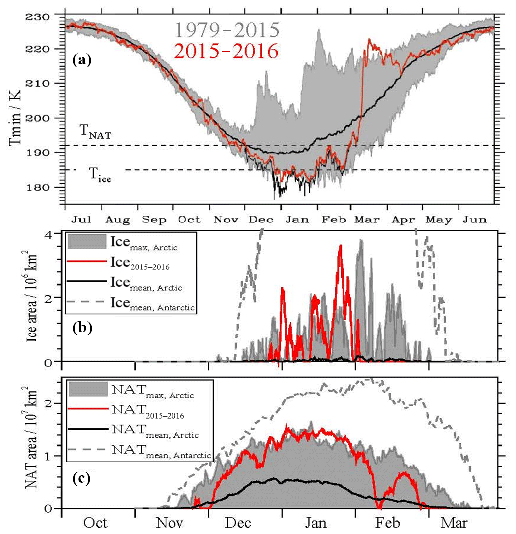
Figure 1Temperature evolution of the 2015–2016 Arctic winter stratosphere (a) 6-hourly ECMWF ERA-Interim reanalysis (Dee et al., 2011) data retrieved at a horizontal resolution of 1∘: minimum temperature Tmin (K) between 65∘ and 90∘ N at the 30 hPa pressure surface. The thick black line denotes the mean values of Tmin averaged during 1979 to 2015, and the shaded areas encompass the minimum and maximum values of Tmin between 1979 and 2015. The red line marks the evolution of Tmin from operational analyses of the IFS cycle 41r1 until 8 March 2016. The thin black line indicates Tmin from the IFS cycle 41r2 in the pre-operational phase from 1 December 2015 to 8 March 2016, retrieved at a resolution of 0.125∘. After 8 March 2016, the black line continues as red curve of the operational IFS cycle 41r2. Tice (Murphy and Koop, 2005) and TNAT (Hanson and Mauersberger, 1988) are calculated using 4.6 ppmv H2O and 7 ppbv HNO3, relevant for the 2015–2016 Arctic vortex conditions (Manney and Lawrence, 2016). (b) Evolution of the vortex area with temperatures below Tice. The black line marks the mean area below Tice (Aice) at 30 hPa pressure (∼21.6 km) between 1979 and 2015. The grey shading indicates maximum and minimum Aice in the same time period. The red line shows the evolution of Aice at the 30 hPa pressure surface in the Arctic winter 2015–2016 of the IFS cycle 41r2. The grey dashed line gives the mean area below Tice at 30 hPa south of 65∘ S from 1979 to 2015, shifted by 6 months to account for seasonality. (c) Same data for NAT.
Therefore, stratospheric temperatures decreased dramatically as derived from the meteorological data of the IFS of the ECMWF numerical weather prediction model. Figure 1a shows the evolution of Tmin at latitudes >65∘ N and at 30 hPa in the Arctic winter 2015–2016 in two resolutions. In December 2015, Tmin decreased below Tice and then remained below Tice from late December 2015 until the end of January 2016. Within the first cold phase, Tmin down to 182 K was detected in the operational IFS analysis with 16 km horizontal resolution. In February 2016, three minor stratospheric warmings influenced the vortex and led to warmer conditions in a coherent but slightly displaced polar vortex (Manney and Lawrence, 2016). Then, the final stratospheric warming resulted in a split of the vortex by mid-March and the subsequent dissipation of the vortices associated with a temperature increase of more than 20 K at 30 hPa in a few days.
The exceptional coldness of the Arctic winter 2015–2016 is also reflected in the fact that by the end of December 2015, Tmin dropped below even the minimum temperatures >65∘ N at 30 hPa ever obtained by the ERA-Interim data record, extending from 1989 to 2016 (Dee et al., 2011). Throughout the Arctic winter 2015–2016, Tmin was continuously lower than the mean temperature of the 36-year ERA-Interim data record (Voigt et al., 2016); see Fig. 1.
To illustrate the effect of mesoscale temperature fluctuations on Tmin, we also show Tmin derived from the IFS cycle 41r2 at ∼8 km horizontal resolution compared to the cycle 41r1 at ∼16 km resolution at 30hPa for the December 2015 to 8 March 2016 time period where both data sets are available. Temperature deviations up to 7 K between the higher- and lower-resolution data sets occurred during the first cold phase with Tmin<Tice in December and early January, as shown in Fig. 1a. At higher resolution, minimum temperatures reach down to 179 K on the 30 hPa level. In the second cold period at the end of January 2016, temperature deviations up to 3 K are found in the higher-resolution data set. Mesoscale gravity wave activity in December and January 2016 is better covered in the higher-resolution data and could have caused this temperature difference (Dörnbrack et al., 2016). On 8 March 2016, the two data sets merge and from then on, ECMWF operational analyses are given at ∼8 km resolution.
At 30 hPa, the area Aice with T>Tice extended over regions up to 3.6×10⁶ km2 (see Fig. 1b), as derived from IFS cycle 41r1 analysis at 16 km resolution. From 18 January until the end of the month, Aice was continuously more than 1 order of magnitude larger than the 36-year average and larger than the maximum of the 36-year ERA-Interim data record. In addition the area ANAT with T<TNAT in January 2016 continuously reached the maximum of the 36-year ERA-Interim data set (Fig. 1c). Generally Aice and ANAT are lower than the mean Antarctic conditions, as given by the dashed grey line in Fig. 1b and c (shifted by 6 months to account for seasonality).
These extremely cold stratospheric winter conditions in the Arctic set the stage for synoptic-scale PSC formation in winter 2015–2016.

Figure 2Curtain plot of the areal occurrence of PSCs in the winter 2015–2016, detected by the CALIOP lidar on board the CALIPSO satellite using the classification from Pitts et al. (2018). (a) Curtain plot of ice PSC occurrence. (b) Curtain plot of NAT and STS mixtures PSC occurrence. Ice PSCs were observed by CALIOP from end of December 2015 until the end of January 2016.
The CALIOP lidar on board the CALIPSO spacecraft detected PSCs from December 2015 to January 2016 (Fig. 2). On 28 January 2016 the CALIOP science data acquisition was suspended due to a spacecraft anomaly. The problem was subsequently resolved and data acquisition began again on 14 March 2016.
Ice PSCs were measured by CALIOP continuously for a month from late December 2015 to late January 2016 (Fig. 2a). The ice PSCs were observed at altitudes between 15 and 26 km during the period with extremely cold temperatures inside the Arctic vortex. The maximum extension of ice PSCs derived from CALIOP Aice,max of (1.75–2.0) × 106 km2 is reached on 30 December 2015. In this phase, the ice PSC formation was predominantly triggered by mountain wave activity and spread out to synoptic scales; see Dörnbrack et al. (2016). Considering the uncertainties in Aice retrieval from the CALIOP data set interpolated to latitude bands, the maximum Aice derived from CALIOP observations agrees reasonably well with maximum Aice derived from weather forecast IFS data of 2.1×10⁶ km2 at 30 hPa (∼21.6 km). Also, the second peak in ice PSC occurrence Aice on 24 January 2016 is captured by the CALIOP routine though with a smaller peak amplitude. A decrease in water vapour concentrations and dehydration due to falling ice crystals has been observed by MLS (Manney and Lawrence, 2016) at these altitudes throughout January 2016. This may explain lower Aice derived from CALIOP data at the end of January compared to Aice derived from in the IFS data set using a fixed H2O mixing ratio of 4.6 ppmv to calculate Aice.
NAT mixtures and STS PSCs were present in the CALIOP data set from early December 2015 until the end of the observation period (Fig. 2b). Summarized, we find strong evidence for the unprecedented existence of widespread ice PSCs in the Arctic winter 2015–2016.
PSCs were detected with the WALES lidar inside the vortex on all six HALO flights between 22 January and 29 February 2016. Before that date, the lidar on HALO was not operational. Due to the strong temperature increase at the end of January and measurement locations of HALO in warmer parts of the vortex, extended ice PSCs were observed by WALES solely on 22 January 2016.
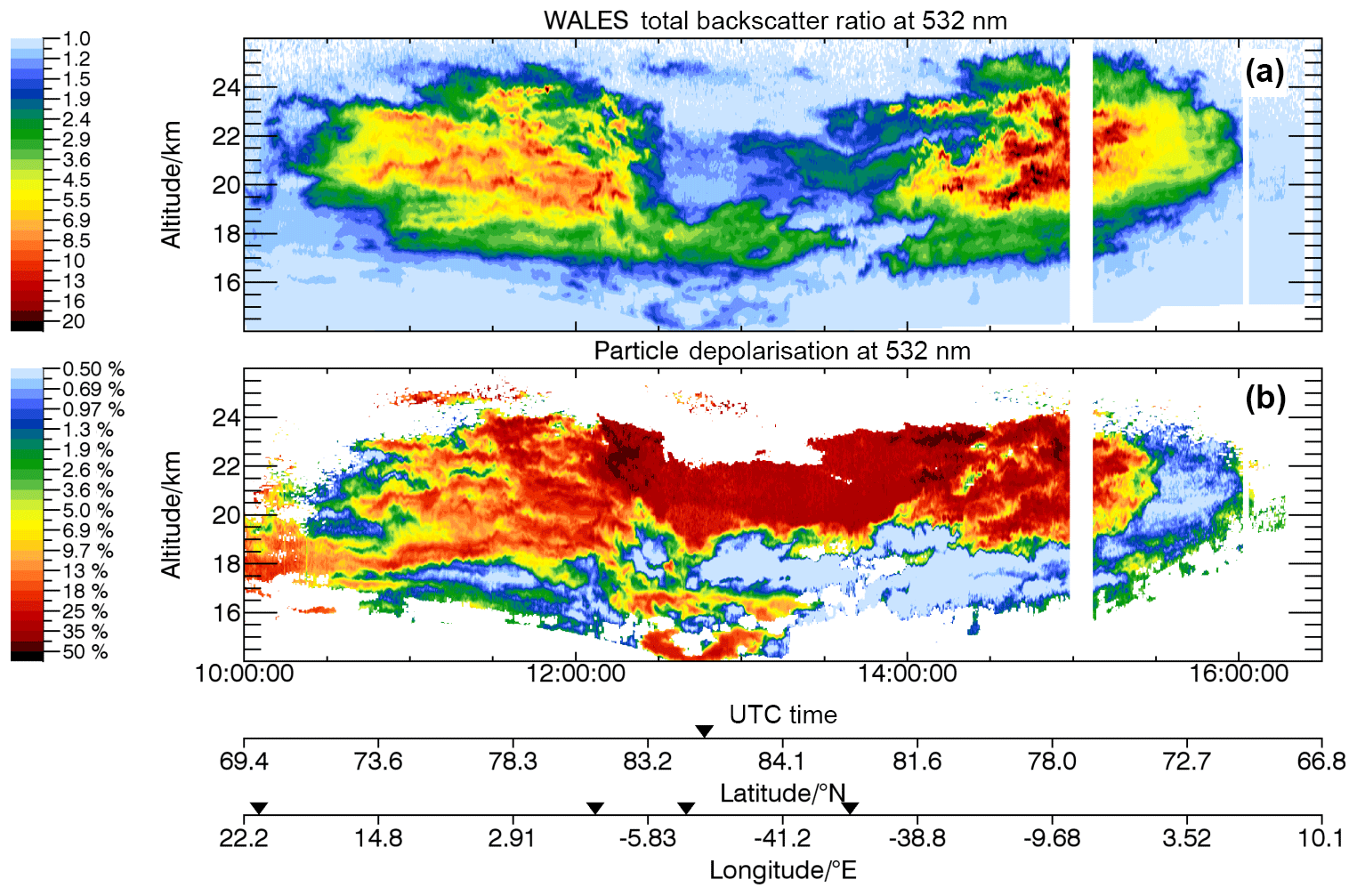
Figure 3Lidar observation of a synoptic-scale polar stratospheric cloud observed on 22 January 2016. (a) Backscatter ratios from the WALES lidar (Wirth et al., 2009) at 532 nm wavelengths during a HALO flight into the Arctic vortex and (b) particle depolarization. The time of the flight as well as latitude and longitude of the HALO flight path are indicated. Turning points of the HALO are marked by triangles.
5.1 Extension of the PSC on 22 January 2016
A large synoptic-scale PSC was measured by WALES during a flight from Kiruna to the northern tip of Greenland on 22 January 2016 as shown in Fig. 3. The PSC extended between 14 and 25 km altitude over a horizontal distance of 2200 km. It was continuously observed within in the Arctic vortex from 72∘ N to the outermost return point at 86∘ N. High backscatter ratios are indicators for the presence of large particle surfaces and high depolarization ratios suggest the presence of solid particles. The co-located measurements of the particle backscatter ratio and depolarization ratio thus allow for a cloud classification into different PSC types.
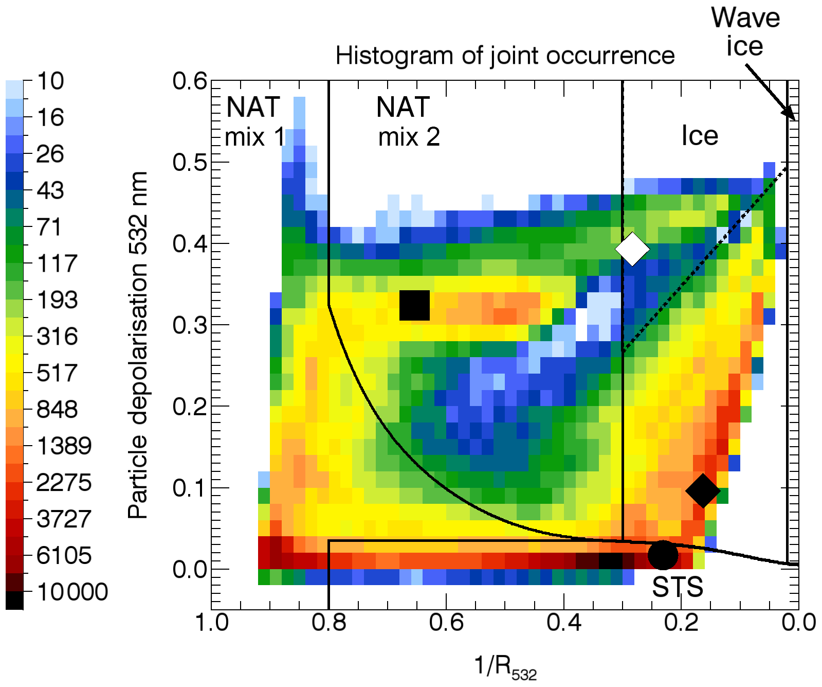
Figure 4Composite 2-dimensional occurrence histogram of the PSC observed on 22 January 2016 shown in Fig. 3 in the 1 ∕ backscatter ratio versus particle depolarization ratio coordinate system. The solid black lines denote the boundaries of the PSC types defined by Pitts et al. (2011), with the threshold between ice and NAT Mix2 . The dotted line separates the high-depol and low-depol ice modes. The symbols indicate the starting points of trajectories within different PSC types (square: NAT Mix2, hollow diamond: high-depol ice, filled diamond: low-depol ice and circle: STS).
5.2 Classification of the PSC measured on 22 January 2016
Figure 4 shows the joint occurrence histogram of the inverse backscatter ratio 1∕R and particle depolarization for the PSC measurements in Fig. 3. The histogram bin size is 0.02×0.02 and the colour scale indicates the number of cloud observations (4 km horizontal by 100 m vertical) falling within each bin. Overlaid are the regions which correspond to different PSC types following Pitts et al. (2011), with two modifications. First, the sub-classification of Mix2 into Mix2-enhanced and normal Mix2 is dropped. Second, the 1∕Rice threshold for ice and NAT regions is set to 0.3. Without the latter change, a substantial part of the branch connecting STS and fully developed ice clouds would have been counted as NAT Mix2 instead of ice, while ice is the more obvious interpretation of the lower branch in the ice class given the form of the joint histogram. The 1∕Rice threshold for ice and NAT regions is discussed in more detail below.
We find two modes in the joint histogram of the ice class, a mode with high particle depolarization ratio (high-depol ice) connected to the NAT Mix2 regime and a mode with lower particle depolarization ratio at the same backscatter ratio (low-depol ice) connected to the STS class. Given several tens of thousands of individual measurement points within the ice class, these two different ice modes can clearly be distinguished. The NAT Mix2 regime with enhanced NAT particle concentrations is strongly populated. In contrast, no observation falls into the wave ice class forming in strong mountain waves.

Figure 5Classification of the synoptic-scale polar stratospheric ice cloud on 22 January 2016 using the classification given in Fig. 3. A synoptic ice PSC (red area) extends over several hundred kilometres above the HALO flight track. The thick black line encloses the low-depol ice mode (see Fig. 4). To the north-west, the ice PSC is embedded in NAT layers (yellow: NAT Mix2, green: NAT Mix1). A liquid STS layer (blue) is located below and to the south-east of the ice PSC. The wave-ice class is not populated. The ending points of the trajectories for ice (high-depol ice (hollow diamond) and low-depol ice (filled diamond)), NAT (square) and STS (circle) given in Fig. 8 are marked. The dashed line shows the Tice contour and the dotted line shows the TNAT contour lines derived from 6-hourly IFS operational weather analysis (cycle 41r2), interpolated to 1-hourly time steps using meteorological forecast data, and the water vapour field measured by WALES as well as the HNO3 field from MLS.
We use the classification by Pitts et al. (2011) and the threshold of of ice versus NAT Mix2 to classify the PSC from Fig. 3. A large ice PSC (red areas in Fig. 5) extends in a cloud layer with a vertical thickness up to 6 km between 18 and 24 km altitude over distances of over 1400 km. The ice PSC is measured twice for more than 1.6 h during the outbound flight leg between 10:34 and 12:30 UTC and during the inbound flight leg between 13:50 and 15:32 UTC. The synoptic-scale ice PSC is observed mainly at temperatures below Tice, as indicated by the dashed contour lines. Here Tice is calculated based on temperature data from the integrated forecast system IFS (cycle 41r1) of ECMWF and measured water vapour mixing ratios. In the northern part of the cloud between 12:30 and 13:50 UTC, the ice PSC is surrounded by NAT Mix2 cloud layers (yellow area) extending above and next to the ice PSC to the north-east. Within the ice PSC, NAT can be masked by the higher optical signal from ice, but may be present. The southernmost part of the PSC observed between 10:15 and 10:34 UTC and again between 15:15 and 16:00 UTC consists of non-depolarizing liquid STS droplets (blue region). The STS layer extends towards the south and below the ice layer.
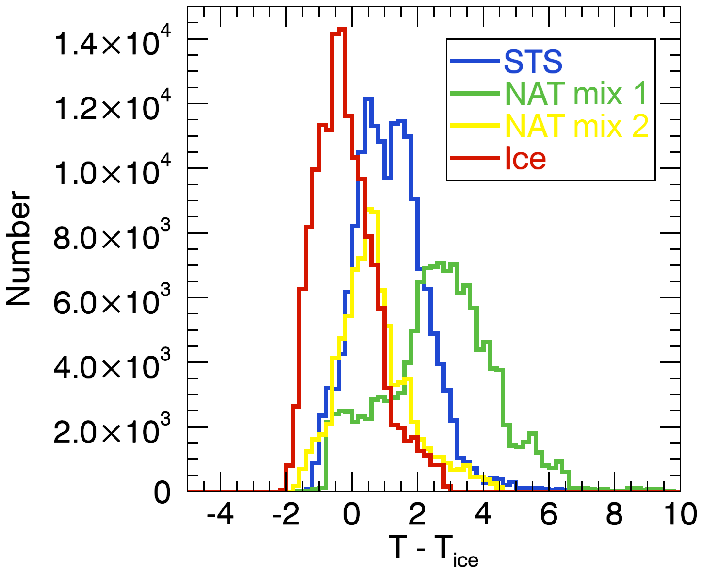
Figure 6Occurrence histogram of ice, NAT Mix2, NAT Mix1 and STS of the 22 January 2016 PSC (Fig. 5) versus temperature difference to Tice.
The ice, NAT Mix and STS occurrence histogram of this PSC is plotted versus temperature difference to Tice in Fig. 6. The peak in ice occurrence is located 0.5 K below Tice. The peak in NAT Mix2 (NAT Mix1) occurrence appears at 0.5 K (3 K) above Tice, while STS occurrence peaks 0.5 to 1.5 K above Tice. The occurrence of ice at temperatures below Tice and of NAT Mix and STS at temperatures above Tice is consistent with their expected temperature range; see also Pitts et al. (2013).
The 1∕Rice threshold of 0.3 best matches the PSC measurements in the low-depol ice mode (see Fig. 4). Also, the PSC area classified as ice agrees best with the ice area derived from numerical weather predictions. For this threshold, the peak of the NAT Mix2 occurrence is located above Tice, while it is located near and below Tice for 1∕Rice of 0.2. Therefore we use the threshold 1∕Rice of 0.3 for the WALES observations on 22 January 2016. The analysis of CALIPSO measurements throughout the winter 2015/16 with changing HNO3 and H2O concentrations requires a variable 1∕Rice threshold as used by Pitts et al. (2018). A detailed investigation of the 1∕Rice threshold is given in the Supplement S1.
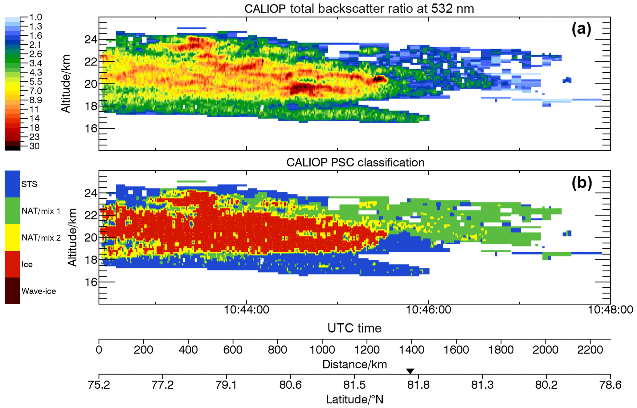
Figure 7CALIPSO PSC measurements on 22 January 2016 near the HALO flight path. (a) Backscatter ratios from CALIPSO at 532 nm wavelengths and (b) PSC type classification from Pitts et al. (2018). The time of the overpass between 10:42 and 10:47 UTC as well as the horizontal distance and the latitude of the CALIPSO footprint are shown. The northernmost turning point of the CALIPSO footprint is marked by the triangle. The CALIPSO footprint is shown in Fig. 8.
The PSC was also measured by CALIPSO on 22 January 2016 between 10:42 and 10:47 UTC. Figure 7 shows the CALIPSO curtain plot measured at the CALIPSO footprint near the HALO flight track shown in Fig. 8. The classification by Pitts et al. (2018) is used to determine the PSC types from CALIPSO. PSC observations by WALES on the slower-flying HALO aircraft lead to the time differences of up to 2 h between the collocated PSC measurements. Similar to the WALES observations, the CALIOP lidar detected an ice PSC between 18 and 24 km altitude with a horizontal extension of about 1200 km. An STS layer is located below the ice cloud and predominantly NAT Mix1 PSCs are measured to the north-west. Only a few NAT Mix2 PSCs were measured by CALIPSO, mainly located at the edge of the ice cloud. Differences in the flight paths of HALO and the CALIPSO footprint explain the lower number of NAT Mix2 PSCs observed by CALIPSO compared to WALES. WALES measured NAT Mix2 mainly north-west of the CALIPSO footprint. Also, a fraction of the low-depol ice mode was located predominantly north-west of the CALIPSO PSC curtain and is therefore barely covered by CALIPSO.

Figure 88-day back-trajectories starting in the different PSC layers measured on 22 January 2016. (a) Temperatures (colour coded) of the back-trajectories derived from the IFS operational analysis (cycle 41r1) starting every 2 min at 21.5∘ altitude in the PSC on 22 January 2016. Four back-trajectories starting in STS (1, circle), low-depol ice (2, LDP-ice, filled diamond), high-depol ice (3, HDP-ice, open diamond) and NAT Mix2 (4, square) are shown as black lines with small symbols marking every 48 h. The HALO flight track is shown as brown line and the CALIPSO footprint as red line. The starting points of the four trajectories are also given in Figs. 4 and 5. The temperature evolution along the four trajectories (STS: blue, NAT: green, LDP-ice: red and HDP-ice: orange) is shown in panel (b) as temperature difference to TNAT for 8 days and (c) as the temperature difference to Tice for 36 h prior to the observation. The ice saturation ratio Sice is given in panel (d). TNAT is calculated from Hanson and Mauersberger (1988) for an altitude-dependent climatological HNO3 profile; H2O, Tice and Sice are calculated from the meteorological data set.
We now discuss PSC formation in two steps based on the WALES lidar and CALIPSO observations combined with trajectory analysis. First we investigate the formation of the ice, NAT and STS layers of the PSC observed on 22 January 2016 using 8-day back-trajectories starting in the different PSC layers at 21.5 km altitude every 2 min. Then we separate the ice PSC into a mode with high particle depolarization (high-depol ice mode) and a mode with low depolarization (low-depol ice mode) as derived from the backscatter ratio to depolarization occurrence histogram in Fig. 4 and discuss ice formation pathways of each ice mode based on domain-filling Lagrangian back-trajectory calculations and their matches with PSC measurements by CALIPSO up to 5 days prior to the ice. We start with the discussion of the formation of the ice, NAT and STS layers of the 22 January 2016 PSC.
6.1 Temperature history of trajectories starting in ice, NAT Mix2 and STS PSC layers
The trajectory calculations were performed using the Hybrid Single-Particle Lagrangian Integrated Trajectory dispersion model (HYSPLIT; Draxler and Hess, 1998) with operational forecast of the deterministic IFS (cycle 41r1 interpolated to 0.25∘×0.25∘) from ECMWF at 3-hourly time steps as meteorological input. We calculate 8-day back-trajectories starting in the PSC observations every 2 min along the HALO flight track (corresponding to approximately 24 km horizontal spacing) at 21.5 km altitude (near 30 hPa) to investigate PSC formation. We further calculate TNAT based on Hanson and Mauersberger (1998) for an altitude-dependent climatological HNO3 profile and use H2O, Tice and the ice saturation ratio Sice from the meteorological data set to discuss ice nucleation pathways. Further we perform sensitivity studies every 2 min at higher and lower altitudes (19, 21 and 23 km) to account for particle sedimentation, which is not included in the simplified trajectory calculations shown here. As a rough estimate, a 10 µm sized ice crystal sediments about 1 km in a day (Fahey et al., 2001). For aspherical particles the sedimentation rates are even lower (Woiwode et al., 2014; Weigel et al., 2014; Woiwode et al., 2016); hence, our simplified calculations generally cover the altitude range of sedimenting PSC particles.
In Fig. 8 we show temperatures of back-trajectories starting every 2 min in the PSC at 21.5 km altitude at the WALES cross section of the outbound flight leg to the north (corresponding to the section from 10:30 to 12:34 UTC in Fig. 5). The air mass trajectories circulate around the pole within these 8 days, and the innermost trajectories (NAT Mix2 at the observation) stay near the Arctic cold pool and remain cold (T<190 K) for 8 days, while the outermost trajectories (STS at the time of observation) encounter higher temperatures (T>198 K) outside of the cold pool. The innermost NAT Mix2 trajectory 4 bypasses Greenland and circulates within the vortex core, while the more southern trajectories are slowly lifted above Greenland. The slow lift contributes to the synoptic cooling within the Arctic cold pool and induces a transient low-amplitude mountain wave temperature disturbance in the lee of the Greenlandic island (dark blue areas in Fig. 8). The synoptic cooling induces the formation of a large-scale ice PSC above and to the east of Greenland within the cold pool of the polar vortex. Teitelbaum et al. (2001) previously investigated the important role of synoptic-scale dynamics for PSC formation.
To investigate PSC formation, four trajectories representative of STS starting at 10:38 UTC (label 1, circle, blue line in panel B and C), in low-depol ice at 11:36 UTC (label 2, filled diamond, red line), in high-depol ice at 12:14 UTC (labels 3, open diamond, orange line) and NAT Mix2 at 12:34 UTC (label 4, square, green line) are selected to represent the temperature histories of the back trajectories of the different PSC types. The numbering of the trajectories is in chronological order during the outbound flight leg and the colour coding in panels (b) and (c) corresponds to the PSC type classification in Fig. 5, with a blue line for STS, a green line for NAT Mix2 and a red line for low-depol ice at the time of the WALES PSC observation. The orange line is used to distinguish the trajectory starting in the high-depol ice mode from the low-depol ice mode (red line). Small symbols denote 48 h time steps along the 8-day back trajectories.
Starting with the outermost STS trajectory, its temperature varies between TNAT−2 K < T < TNAT+11 K for 6.5 days as the trajectories circulate mainly out of the Arctic cold pool. Then, the temperature decreases below TNAT∼36 h and below Tice∼16 h prior to the observation before increasing to Tice+2 K at the time of STS detection. The temperature at the time of observation is within the STS temperature range.
Slightly further to the north, the low-depol ice mode back-trajectory (red line) is located at the edge of the cold pool, with temperatures oscillating between TNAT−6 K < T < TNAT+6 K for 7 days. The temperatures decrease below TNAT∼36 h and finally below Tice∼16 h prior to the observation. At the time of observation of the low-depol ice mode, the trajectories' temperatures are near and below Tice, explaining the detection of ice PSCs. The ice saturation ratio Sice increases to 1.4 and varies between 1.4 and 0.92 in the last 16 h prior to observation. While Sice<1.4 does not allow for homogeneous ice nucleation (Koop et al., 2000; Murphy and Koop, 2005), heterogeneous nucleation (e.g. Hoose and Möhler, 2012) could explain ice formation in this case. Thereby meteoric material (Cziczo et al., 2001; Voigt et al., 2005; Curtius et al., 2005) probably embedded in STS could serve as ice nuclei. This has been suggested by Engel et al. (2013) to explain the observation of an Arctic ice PSC in 2010. Small-scale temperature fluctuations might be present in our case, but cannot be resolved in the meteorological model.
In contrast, the northernmost NAT Mix2 trajectory (4, green line) circulates within the cold pool at temperatures TNAT−8 K < T < TNAT−4 K for 8 days without passing over Greenland. The temperatures remain above Tice throughout that period and T>Tice at the time of observations, consistent with NAT. Homogeneous NAT nucleation rates (Knopf et al., 2002) are too low to support homogeneous NAT nucleation in this case. In contrast, NAT nucleation rates on meteoric dust (Voigt et al., 2005; Grooß et al., 2005, 2014; Hoyle et al., 2013) may explain the formation of NAT within a few days and are consistent with the observations of NAT.
Similarly, the trajectory of the high-depol ice mode (3, orange line) circulates within the polar vortex for 8 days at temperatures between TNAT−10 K < T < TNAT. However, when passing over Greenland, the high-depol ice trajectories decrease below Tice∼10 h prior to the observation. The temperature is Tice−2 K at the time of observation of high-depol ice and Sice increases up to 1.2. This temperature history supports heterogeneous ice nucleation. Laboratory measurements of heterogeneous ice nucleation (Hoose and Möhler, 2012) were performed for a suite of different ice nuclei at temperatures down to 213 K, hence above PSC formation temperatures. Meteoric dust could potentially serve as ice nuclei in the stratosphere at Sice∼1.2; however, surface area densities of meteoritic material are significantly smaller than those of NAT PSCs. Therefore we investigate the possibility of ice nucleation on NAT and NAT serving as ice nuclei.
The temperature history of the high-depol ice trajectory also remains below the existence temperature of NAD ( K; Voigt et al., 2005) for about a week. The formation of NAD from binary nitric acid water solutions has been observed in the laboratory (e.g. Knopf et al., 2002; Wagner et al., 2005; Stetzer et al., 2006), but homogeneous nucleation rates are too low to explain denitrification (Knopf et al., 2002). Also, pseudo-heterogeneous nucleation rates (Knopf, 2006) cannot explain atmospheric nitric acid hydrate particle number densities. Möhler et al. (2006) suggest that ambient supersaturations with respect to NAD of 8 to 9 are required over days to explain NAD particle nucleation at number densities, which can be detected with current instrumentations. Furthermore, a phase change from NAD into NAT or a nucleation of NAT on NAD under atmospheric conditions is not supported by laboratory experiments (Tizek et al., 2004; Stetzer et al., 2006). Observational evidence for the presence of NAD in the atmosphere is missing so far; e.g. Höpfner et al. (2006a) found no spectroscopic evidence for the presence of NAD from MIPAS observations of PSCs over Antarctica. Therefore, we focus the discussion on ice nucleation on NAT in our study.
6.2 Ice nucleation pathways
The existence of the two ice modes with high and low particle depolarization ratios (Fig. 4) in combination with the trajectory analysis suggests two different ice nucleation pathways. (1) Ice nucleation in STS may account for the low-depol ice mode. Inclusions of meteoric material in STS as suggested by Engel et al. (2013) are below the detection limit of the WALES lidar but may be present. (2) A second ice nucleation pathway is required to explain the formation of the high-depol ice mode. The long time period below TNAT prior to the observation and the similarity of the NAT Mix2 and the high-depol ice trajectories (except for the last hours, where the high-depol ice trajectories are ice supersaturated) points to ice nucleation on pre-existing NAT particles.
The hypothesis of ice nucleation on NAT ice is investigated in more detail using a Lagrangian match approach of 5-day back-trajectories matched with CALIPSO PSC measurements, similar to the method outlined by Santee et al. (2002). Domain-filling trajectories starting in the WALES ice PSC observations are calculated every 2 min along the flight path from 10:30 UTC until 16:00 UTC (corresponding to ∼24 km distance) at 15 different altitude levels with 500 m spacing between 17 and 24 km. Thus a total of 2490 trajectories are derived. We match the Lagrangian trajectories with all CALIPSO PSC curtain plots measured north of 60∘ N within 5 days prior to 22 January 2016. The study of Pitts et al. (2018) is used to classify the PSC types within the CALIPSO curtains. A match is defined as a point along a trajectory lying within a given horizontal distance limit from one of the CALIOP footprints at the same time. To yield a statistically significant number of matches we set a distance limit of 100 km. A threshold of this order is justified by the limited accuracy of the trajectory calculations, too. In addition, to make the spatial resolution comparable with the initial spacing of the trajectories' starting points, 15 CALIPSO PSC data points with 3×180 m vertical and 5×5 km horizontal distance are grouped to smooth variations in the PSC type classification in nearby data points at the edge of PSC layers. A match point is classified as ice, NAT or STS, if >50 % of the CALIPSO pixel array is classified as the respective PSC type. The match method is selected to investigate whether a different PSC type was present before the high-depol and low-depol ice PSC observation by WALES on 22 January 2016. If so, the analysis indicates which PSC type has been detected prior to high-depol or low-depol ice.
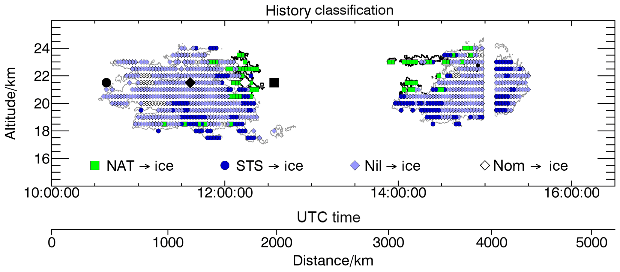
Figure 9PSC type measured by CALIPSO prior to ice on match points with 5-day back-trajectories. Green squares indicate that NAT has been measured by CALIPSO prior to ice, blue circles indicate STS prior to ice, and light blue diamonds (nil) indicate that no PSC has been observed and (nom) that no match point of the trajectories and the CALIPSO curtain exist within 5 days. NAT has been detected by CALIPSO prior to the high-depol ice mode measured by WALES (thick black contour line) and predominantly STS or no PSC have been detected prior to the low-depol ice mode measured by WALES (thin grey contour line). UTC times of the WALES ice PSC observations and the horizontal distance are given. The starting points of the four trajectories from Fig. 8 are indicated by the black and white symbols.
The trajectories are classified using the following criteria: (1) NAT has been measured in the CALIPSO curtain–trajectory match point prior to ice measured by WALES, or prior to the last CALIPSO match with ice on the same trajectory; (2) STS has been observed in the CALIPSO curtain–trajectory match point prior to ice; (3) no PSC (nil) has been observed in the match point prior to ice; or (4) no match (nom) has occurred along the trajectories.
The result of the match analysis is presented in Fig. 9 overlaid on the ice PSC contour of the 22 January PSC. The result is evident: NAT has been measured by CALIPSO on all match points directly prior to the high-depol ice mode. Thus the CALIPSO-trajectory match analysis delivers strong evidence for ice nucleation on NAT. Ice could have nucleated on pre-existing NAT particles, which could also explain the high particle depolarization ratio of the ice mode. In contrast, predominantly STS or no PSC has been observed on the match points prior to the low-depol ice mode. We note the possibility that due to fast evaporation times, STS might have existed along the trajectories classified as nil, but was not present at the time of the CALIPSO overpass. Only a few trajectories have no match points with CALIPSO.
To summarize, we find strong evidence for ice nucleation on NAT. Ice nucleated on NAT may produce ice particles with higher particle depolarization ratios. In contrast, the low-depol ice mode can be explained by ice nucleation in STS, possibly with solid meteoric inclusions as suggested by Engel et al. (2013). Ice nucleation in STS may lead to lower particle depolarization ratios of the ice mode. These two ice formation pathways would be consistent with the CALIPSO and WALES observations combined with results from domain-filling trajectory analysis.
Extremely low temperatures existed in the Arctic stratospheric winter 2015–2016 because low planetary wave activity resulted in a stable vortex. Synoptic-scale ice PSCs formed in late December 2015 and persisted throughout January, as observed by the CALIOP lidar on board the CALIPSO satellite. The sedimentation of the ice PSC particles led to significant dehydration (Khosrawi et al., 2017). From January to early March 2016, water vapour data and MLS data show severe dehydration between 400 and 500 K potential temperatures (Manney and Lawrence, 2016). In addition, ice PSCs can serve as efficient transporters for nitric acid incorporated into ice (Voigt et al., 2007). Large ice particles sediment faster than smaller NAT particles and therefore ice can lead to efficient denitrification at PSC altitudes. Massive denitrification has been measured by MLS with an onset in mid-December 2015 throughout the Arctic winter (Manney and Lawrence, 2016; Khosrawi et al., 2017).
We use high-resolution WALES lidar measurements of a large-scale ice PSC observed on 22 January 2016 in combination with domain-filling back-trajectories matched to CALIPSO PSC observations to investigate ice nucleation pathways. Two distinct modes with high and low particle depolarization in the ice PSC occurrence histogram suggest different particle size distributions and shapes in the two modes, possibly linked to two ice formation pathways. Ice nucleation in STS, possibly with meteoric inclusions as suggested by Engel et al. (2013), may lead to the ice mode with low particle depolarization ratios. In addition, NAT has been detected by CALIPSO on trajectory match points prior to high-depol ice. Thus, ice formation on NAT could lead to the ice mode with higher particle depolarization ratios. While the low-depol STS-ice branch is frequently populated in space-borne CALIOP lidar data, the high-depol NAT Mix2-ice branch is less frequently observed by CALIOP in Arctic or Antarctic PSC measurements (Pitts et al., 2013, 2018). Larger noise in the satellite data with CALIPSO travelling at an orbit near 700 km and a higher detection limit of the CALIOP lidar data compared to the WALES measurements on aircraft cruising at 14 km altitude may contribute to this difference.
Lambert et al. (2012) investigate PSC occurrence in the Antarctic in early winter from 11 to 30 June 2008 based on CALIOP and MLS observations. They detect a NAT Mix2-type PSC linked to the high-depol ice regime. They also note that the conservative estimate by Pitts et al. (2013) of the threshold may lead to a mis-classification of the ice PSC with respect to the NAT MIX2 regime. The threshold of 0.3 provides a better fit to their observation. Similarly to the Arctic case, the NAT Mix2 trajectories remain 3 to 5 K below TNAT for 5 days, suggesting heterogeneous NAT nucleation. Ice formation is not investigated in detail for this Antarctic PSC, although ice is present. The low-depol ice mode is sparsely populated, supporting the hypothesis of ice nucleation on NAT in the Antarctic June 2008 PSC. Further high-resolution lidar observations are required to estimate the global occurrence of the high-depol ice mode. These observations could then help to evaluate the importance of the suggested NAT-ice nucleation pathway in other regions of the atmosphere. In addition, combined lidar and in situ observations from aircraft (e.g. Fahey et al., 2001; Northway et al., 2002) could help to answer the question on the abundance of the NAT Mix2, which might include aspherical NAT particles as observed by Molleker et al. (2014) and Woiwode et al. (2016).
The NAT crystal has a stoichiometry of 1 HNO3 × 3 H2O molecules and exists in α−NAT or β−NAT crystal structure (Iannarelli and Rossi, 2015). Compared to liquid aerosol or meteoric particles, the NAT crystal structure is more similar to that of ice, and therefore NAT readily nucleates on ice, as is frequently observed in laboratory experiments (Hanson and Mauersberger, 1988; Iannarelli and Rossi, 2015; Gao et al., 2016; Weiss et al., 2016) and in mountain wave ice PSCs (Carslaw et al., 2002; Fueglistaler et al., 2002a, b; Luo et al., 2003; Voigt et al., 2003). Vice versa, we propose here that ice may nucleate on NAT. This pathway has been suggested in early PSC studies (e.g. Peter, 1997) and has later been neglected. Here, we find evidence for ice nucleation on NAT and elucidate its importance in the polar lower stratosphere. Direct laboratory measurements of the nucleation rate of ice on NAT are missing (Koop et al., 1997) and would be required to provide further evidence of the suggested ice nucleation process.
Ice nucleation on NAT may be important in the tropical tropopause region, where the existence of a NAT belt and cirrus has been detected by in situ measurements (Popp et al., 2007; Voigt et al., 2008). Also, CALIPSO measurements showed indications for the existence of NAT in the tropics (Chepfer and Noel, 2009), although Pitts et al. (2009) argue that mixtures of liquid aerosols and thin cirrus instead might have been misinterpreted as NAT-like particles in the tropics. Based on the observational data set, the ice nucleation rate on NAT could be parameterized and implemented in a large-scale model in order to assess the global relevance the different ice nucleation pathways in different regions of the atmosphere.
The observational data are available at https://halo-db.pa.op.dlr.de (DLR, 2017). Operational meteorological analyses are achieved in the MARS archive at ECMWF (https://www.ecmwf.int/en/forecasts/documentation-and-support/changes-ecmwf-model/ifs-documentation, ECMWF, 2017a), and ERA-Interim data were taken from https://www.ecmwf.int/en/research/climate-reanalysis/era-interim (ECMWF, 2017b).
The supplement related to this article is available online at: https://doi.org/10.5194/acp-18-15623-2018-supplement.
CV performed the scientific study and wrote the paper. AD and BE analysed the meteorological conditions for the Arctic winter 2016. MW and SG performed the HALO lidar measurements and data evaluation. MP and LP evaluated CALIPSO data. RB made the HYSPLIT trajectory calculations. BMS, WW and HO were the coordinators of the POLSTRACC campaign. All authors contributed to the paper.
The authors declare that they have no conflict of interest.
This article is part of the special issue “The Polar Stratosphere in a Changing Climate (POLSTRACC) (ACP/AMT inter-journal SI)”. It is not associated with a conference.
We thank the DLR flight department for excellent support of the campaign.
Further we thank Helmut Ziereis, Tina Jurkat-Witschas and Stefan Kaufmann for helpful comments on
the paper. Support for the campaign was provided by the HALO-SPP 1294
programme and the Helmholtz society via the ATMO programme. CV has been funded by
the Helmholtz society under contact no. W2/W3-060 and by DFG contract no.
VO1504/4-1, and BE by DFG contract no DO1400/6-1. Support for MP and LP is
provided by the NASA CALIPSO/CloudSat Science Team.
The article processing charges for this open-access
publication were covered by a Research
Centre
of the Helmholtz Association.
Edited by: Robyn Schofield
Reviewed by: Michael Fromm and two anonymous referees
Achtert, P. and Tesche, M.: Assessing lidar-based classification schemes for polar stratospheric clouds based on 16 years of measurements at Esrange, Sweden, J. Geophys. Res.-Atmos., 119, 1386–1405, https://doi.org/10.1002/2013JD020355, 2014.
Berrisford, P., Dee, D., Poli, P., Brugge, R., Fielding, K., Fuentes, M., Kallberg, P., Kobayashi, S., Uppala, S., and Simmons, A.: The ERA-Interim archive Version 2.0, ERA Report Series 1, ECMWF, Shinfield Park, Reading, UK, 2011.
Carslaw, K. S., Luo, B. P., Clegg, S. L., Peter, Th., Brimblecombe, P., and Crutzen, P. J.: Stratospheric aerosol growth and HNO3 and water uptake by liquid particles, Geophys. Res. Lett., 21, 2479–2482, 1994.
Carslaw, K. S., Kettleborough, J. A., Northway, M. J., Davies, S., Gao, R. S., Fahey, D. W., Baumgardner, D. G., Chipperfield, M. P., and Kleinbohl, A.: A vortex-scale simulation of the growth and sedimentation of large nitric acid hydrate particles, J. Geophys. Res.-Atmos., 107, SOL 43-1–SOL 43-16, https://doi.org/10.1029/2001jd000467, 2002.
Chepfer, H. and Noel, V.: A tropical “NAT-like” belt observed from space, Geophys. Res. Lett., 36, L03813, https://doi.org/10.1029/2008GL036289, 2009.
Crutzen, P. J. and Arnold, F.: Nitric-Acid Cloud Formation in the Cold Antarctic Stratosphere – a Major Cause for the Springtime Ozone Hole, Nature, 324, 651–655, https://doi.org/10.1038/324651a0, 1986.
Curtius, J., Weigel, R., Vössing, H.-J., Wernli, H., Werner, A., Volk, C.-M., Konopka, P., Krebsbach, M., Schiller, C., Roiger, A., Schlager, H., Dreiling, V., and Borrmann, S.: Observations of meteoric material and implications for aerosol nucleation in the winter Arctic lower stratosphere derived from in situ particle measurements, Atmos. Chem. Phys., 5, 3053–3069, https://doi.org/10.5194/acp-5-3053-2005, 2005.
Cziczo, D. J., Thomson, D. S., and Murphy, D. M.: Ablation, flux, and atmospheric implications of meteors inferred from stratospheric aerosol, Science, 291, 1772–1775, https://doi.org/10.1126/science.1057737, 2001.
Dee, D. P., Uppala, S. M., Simmons, A. J., Berrisford, P., Poli, P., Kobayashi, S., Andrae, U., Balmaseda, M. A., Balsamo, G., Bauer, P., Bechtold, P., Beljaars, A. C. M., van de Berg, L., Bidlot, J., Bormann, N., Delsol, C., Dragani, R., Fuentes, M., Geer, A. J., Haimberger, L., Healy, S. B., Hersbach, H., Holm, E. V., Isaksen, L., Kallberg, P., Kohler, M., Matricardi, M., McNally, A. P., Monge-Sanz, B. M., Morcrette, J. J., Park, B. K., Peubey, C., de Rosnay, P., Tavolato, C., Thepaut, J. N., and Vitart, F.: The ERA-Interim reanalysis: configuration and performance of the data assimilation system, Q. J. Roy. Meteor. Soc., 137, 553–597, https://doi.org/10.1002/qj.828, 2011.
DLR: #4938, PGS_09_20160122_WALES_ADEP532_V2.nc, available at: https://halo-db.pa.op.dlr.de (last access: 26 October 2018), 2017.
Dörnbrack, A., Birner, T., Fix, A., Flentje, H., Meister, A., Schmid, H., Browell, E. V., and Mahoney, M. J.: Evidence for inertia gravity waves forming polar stratospheric clouds over Scandinavia, J. Geophys. Res.-Atmos., 107, SOL 30-1–SOL 30-18, https://doi.org/10.1029/2001jd000452, 2002.
Dörnbrack, A., Gisinger, S., Pitts, M. C., Poole, L. R., and Maturilli, M.: Multilevel cloud structures over Svalbard, Mon. Weather Rev., 145, 1149–1159, https://doi.org/10.1175/mwr-d-16-0214.1, 2016.
Draxler, R. R. and Hess, G. D.: An overview of the HYSPLIT4 modeling system of trajectories, dispersion, and deposition, Aust. Meteor. Mag., 47, 295–308, 1998.
Drdla, K. and Müller, R.: Temperature thresholds for chlorine activation and ozone loss in the polar stratosphere, Ann. Geophys., 30, 1055–1073, https://doi.org/10.5194/angeo-30-1055-2012, 2012.
Dye, J. E., Baumgardner, D., Gandrud, B. W., Kawa, S. R., Kelly, K. K., Loewenstein, M., Ferry, G. V., Chan, K. R., and Gary, B. L.: Particle-Size Distributions in Arctic Polar Stratospheric Clouds, Growth and Freezing of Sulfuric-Acid Droplets, and Implications for Cloud Formation, J. Geophys. Res.-Atmos., 97, 8015–8034, https://doi.org/10.1029/91JD02740, 1992.
ECMWF: CY41R1, available at: https://www.ecmwf.int/en/forecasts/documentation-and-support/changes-ecmwf-model/ifs-documentation (last access: 26 October 2018), 2017a.
ECMWF: CY31R2, available at: https://www.ecmwf.int/en/research/climate-reanalysis/era-interim (last access: 26 October 2018), 2017b.
Engel, I., Luo, B. P., Pitts, M. C., Poole, L. R., Hoyle, C. R., Grooss, J. U., Dornbrack, A., and Peter, T.: Heterogeneous formation of polar stratospheric clouds – Part 2: Nucleation of ice on synoptic scales, Atmos. Chem. Phys., 13, 10769–10785, https://doi.org/10.5194/acp-13-10769-2013, 2013.
Esselborn, M., Wirth, M., Fix, A., Tesche, M., and Ehret, G.: Airborne high spectral resolution lidar for measuring aerosol extinction and backscatter coefficients, Appl. Opt., 47, 346–358, https://doi.org/10.1364/AO.47.000346, 2008.
Fahey, D. W., Kelly, K. K., Kawa, S. R., Tuck, A. F., Loewenstein, M., Chan, K. R., and Heidt, L. E.: Observations of denitrification and dehydration in the winter polar stratospheres, Nature, 344, 321–324, https://doi.org/10.1038/344321a0, 1990.
Fahey, D. W., Gao, R. S., Carslaw, K. S., Kettleborough, J., Popp, P. J., Northway, M. J., Holecek, J. C., Ciciora, S. C., McLaughlin, R. J., Thompson, T. L., Winkler, R. H., Baumgardner, D. G., Gandrud, B., Wennberg, P. O., Dhaniyala, S., McKinney, K., Peter, T., Salawitch, R. J., Bui, T. P., Elkins, J. W., Webster, C. R., Atlas, E. L., Jost, H., Wilson, J. C., Herman, R. L., Kleinbohl, A., and von Konig, M.: The detection of large HNO3-containing particles in the winter arctic stratosphere, Science, 291, 1026–1031, https://doi.org/10.1126/science.1057265, 2001.
Farman, J. C., Gardiner, B. G., and Shanklin, J. D.: Large losses of total ozone in Antarctica reveal seasonal ClO_x/NO_x interaction, Nature, 315, 207–210, https://doi.org/10.1038/315207a0, 1985.
Freudenthaler, V., Esselborn, M., Wiegner, M., Heese, B., Tesche, M., Ansmann, A., Müller, D., Althausen, D., Wirth, M., Fix, A., Ehret, G., Knippertz, P., Toledano, C., Gasteiger, J., Garhammer, M., and Seefeldner, M.: Depolarization ratio profiling at several wavelengths in pure Saharan dust during SAMUM 2006, Tellus B, 61, 165–179, https://doi.org/10.1111/j.1600-0889.2008.00396.x, 2009.
Fueglistaler, S., Luo, B. P., Buss, S., Wernli, H., Voigt, C., Muller, M., Neuber, R., Hostetler, C. A., Poole, L. R., Flentje, H., Fahey, D. W., Northway, M. J., and Peter, T.: Large NAT particle formation by mother clouds: Analysis of SOLVE/THESEO-2000 observations, Geophys. Res. Lett., 29, 52-1–52-4, https://doi.org/10.1029/2001gl014548, 2002a.
Fueglistaler, S., Luo, B. P., Voigt, C., Carslaw, K. S., and Peter, Th.: NAT-rock formation by mother clouds: a microphysical model study, Atmos. Chem. Phys., 2, 93–98, https://doi.org/10.5194/acp-2-93-2002, 2002b.
Gao, R.-S, Gierczak, T., Thornberry, T. D., Rollins, A. W., Burkholder, J. B., Telg, H., Voigt, C., Peter, T., and Fahey, D. W.: A Persistent Water-Nitric Acid Condensate with Saturation Water Vapor Pressure Greater Than Hexagonal Ice, J. Phys. Chem. A, https://doi.org/10.1021/acs.jpca.5b06357, 2015.
Grooß, J.-U., Günther, G., Müller, R., Konopka, P., Bausch, S., Schlager, H., Voigt, C., Volk, C. M., and Toon, G. C.: Simulation of denitrification and ozone loss for the Arctic winter 2002/2003, Atmos. Chem. Phys., 5, 1437–1448, https://doi.org/10.5194/acp-5-1437-2005, 2005.
Grooß, J.-U., Engel, I., Borrmann, S., Frey, W., Günther, G., Hoyle, C. R., Kivi, R., Luo, B. P., Molleker, S., Peter, T., Pitts, M. C., Schlager, H., Stiller, G., Vömel, H., Walker, K. A., and Müller, R.: Nitric acid trihydrate nucleation and denitrification in the Arctic stratosphere, Atmos. Chem. Phys., 14, 1055–1073, https://doi.org/10.5194/acp-14-1055-2014, 2014.
Groß, S., Wirth, M., Schäfler, A., Fix, A., Kaufmann, S., and Voigt, C.: Potential of airborne lidar measurements for cirrus cloud studies, Atmos. Meas. Tech., 7, 2745–2755, https://doi.org/10.5194/amt-7-2745-2014, 2014.
Hanson, D. and Mauersberger, K.: Laboratory Studies of the Nitric-Acid Trihydrate – Implications for the South Polar Stratosphere, Geophys. Res. Lett., 15, 855–858, https://doi.org/10.1029/Gl015i008p00855, 1988.
Hanson, D. R. and Ravishankara, A. R.: Investigation of the Reactive and Nonreactive Processes Involving ClONO2 and HCl on Water and Nitric Acid Doped Ice, J. Phys. Chem., 96, 2682–2691, https://doi.org/10.1021/J100185a052, 1992.
Hólm, E., Forbes, R., Lang, S., Magnusson, L., and Malardel, S.: New model cycle brings higher resolution, ECMWF Newsletter, No. 147, ECMWF, Reading, United Kingdom, 14–19, 2016, available at: http://www.ecmwf.int/sites/default/files/elibrary/2016/16299-newsletter-no147-spring-2016.pdf (last access: June 2017), 2016.
Hoose, C. and Möhler, O.: Heterogeneous ice nucleation on atmospheric aerosols: a review of results from laboratory experiments, Atmos. Chem. Phys., 12, 9817–9854, https://doi.org/10.5194/acp-12-9817-2012, 2012.
Höpfner, M., Luo, B. P., Massoli, P., Cairo, F., Spang, R., Snels, M., Di Donfrancesco, G., Stiller, G., von Clarmann, T., Fischer, H., and Biermann, U.: Spectroscopic evidence for NAT, STS, and ice in MIPAS infrared limb emission measurements of polar stratospheric clouds, Atmos. Chem. Phys., 6, 1201–1219, https://doi.org/10.5194/acp-6-1201-2006, 2006a.
Höpfner, M., Larsen, N., Spang, R., Luo, B. P., Ma, J., Svendsen, S. H., Eckermann, S. D., Knudsen, B., Massoli, P., Cairo, F., Stiller, G., v. Clarmann, T., and Fischer, H.: MIPAS detects Antarctic stratospheric belt of NAT PSCs caused by mountain waves, Atmos. Chem. Phys., 6, 1221–1230, https://doi.org/10.5194/acp-6-1221-2006, 2006b.
Hoyle, C. R., Engel, I., Luo, B. P., Pitts, M. C., Poole, L. R., Grooss, J. U., and Peter, T.: Heterogeneous formation of polar stratospheric clouds – Part 1: Nucleation of nitric acid trihydrate (NAT), Atmos. Chem. Phys., 13, 9577–9595, https://doi.org/10.5194/acp-13-9577-2013, 2013.
Hunt, W. H., Winker, D. M., Vaughan, M. A., Powell, K. A., Lucker, P. L., and Weimer, C.: CALIPSO lidar description and performance assessment, J. Atmos. Oceanic Technol., 26, 1214–1228, https://doi.org/10.1175/2009JTECHA1223.1, 2009.
Iannarelli, R. and Rossi, M. J.: The mid-IR Absorption Cross Sections of alpha- and beta-NAT (HNO3 * 3H2O) in the range 170 to 185K and of metastable NAD (HNO3 * 2H2O) in the range 172 to 182K, J. Geophys. Res.-Atmos., 120, 11707–11727, https://doi.org/10.1002/2015JD023903, 2015.
Khosrawi, F., Kirner, O., Sinnhuber, B.-M., Johansson, S., Höpfner, M., Santee, M. L., Froidevaux, L., Ungermann, J., Ruhnke, R., Woiwode, W., Oelhaf, H., and Braesicke, P.: Denitrification, dehydration and ozone loss during the 2015/2016 Arctic winter 2015/2016, Atmos. Chem. Phys., 17, 12893–12910 https://doi.org/10.5194/acp-17-12893-2017, 2017.
Knopf, D. A.: Do NAD and NAT Form in Liquid Stratospheric Aerosols by Pseudoheterogeneous Nucleation?, The J. Phys. Chem. A, 110, 5745–5750, https://doi.org/10.1021/jp055376j, 2006.
Knopf, D. A., Koop, T., Luo, B. P., Weers, U. G., and Peter, T.: Homogeneous nucleation of NAD and NAT in liquid stratospheric aerosols: insufficient to explain denitrification, Atmos. Chem. Phys., 2, 207–214, https://doi.org/10.5194/acp-2-207-2002, 2002.
Koop, T., Carslaw, K. S., and Peter, T.: Thermodynamic stability and phase transitions of PSC particles, Geophys. Res. Lett., 24, 2199–2202, https://doi.org/10.1029/97gl02148, 1997.
Koop, T., Luo, B., Tsias, A., and Peter, T.: Water activity as the determinant for homogeneous ice nucleation in aqueous sloutions, Nature, 406, 611–614, https://doi.org/10.1038/35020537, 2000.
Lambert, A., Santee, M. L., Wu, D. L., and Chae, J. H.: A-train CALIOP and MLS observations of early winter Antarctic polar stratospheric clouds and nitric acid in 2008, Atmos. Chem. Phys., 12, 2899–2931, https://doi.org/10.5194/acp-12-2899-2012, 2012.
Luo, B. P., Voigt, C., Fueglistaler, S., and Peter, T.: Extreme NAT supersaturations in mountain wave ice PSCs: A clue to NAT formation, J. Geophys. Res.-Atmos., 108, 4441, https://doi.org/10.1029/2002jd003104, 2003.
Malardel, S., and Wedi, N. P.: How does subgrid-scale parametrization influence nonlinear spectral energy fluxes in global NWP models? J. Geophys. Res.-Atmos., 121, 5395–5410, https://doi.org/10.1002/2015JD023970, 2016.
Manney, G. and Lawrence, Z. D.: The major stratospheric final warming in 2016: Dispersal of vortex air and termination of Arctic chemical ozone loss, Atmos. Chem. Phys., 15371–15396, https://doi.org/10.5194/acp-16-15371-2016, 2016.
Manney, G. L., Santee, M. L., Rex, M., Livesey, N. J., Pitts, M. C., Veefkind, P., Nash, E. R., Wohltmann, I., Lehmann, R., Froidevaux, L., Poole, L. R., Schoeberl, M. R., Haffner, D. P., Davies, J., Dorokhov, V., Gernandt, H., Johnson, B., Kivi, R., Kyro, E., Larsen, N., Levelt, P. F., Makshtas, A., McElroy, C. T., Nakajima, H., Parrondo, M. C., Tarasick, D. W., von der Gathen, P., Walker, K. A., and Zinoviev, N. S.: Unprecedented Arctic ozone loss in 2011, Nature, 478, 465–469, https://doi.org/10.1038/nature10556, 2011.
Matthias, V., Dörnbrack, A., and Stober, G.: The extraordinary strong and cold polar vortex in the early northern winter 2015/2016, Geophys. Res. Lett., 43, 12287–12294, https://doi.org/10.1002/2016GL071676, 2016.
Möhler, O., Bunz, H., and Stetzer, O.: Homogeneous nucleation rates of nitric acid dihydrate (NAD) at simulated stratospheric conditions – Part II: Modelling, Atmos. Chem. Phys., 6, 3035–3047, https://doi.org/10.5194/acp-6-3035-2006, 2006.
Molleker, S., Borrmann, S., Schlager, H., Luo, B., Frey, W., Klingebiel, M., Weigel, R., Ebert, M., Mitev, V., Matthey, R., Woiwode, W., Oelhaf, H., Dörnbrack, A., Stratmann, G., Grooß, J.-U., Günther, G., Vogel, B., Müller, R., Krämer, M., Meyer, J., and Cairo, F.: Microphysical properties of synoptic-scale polar stratospheric clouds: in situ measurements of unexpectedly large HNO3-containing particles in the Arctic vortex, Atmos. Chem. Phys., 14, 10785–10801, https://doi.org/10.5194/acp-14-10785-2014, 2014.
Murphy, D. M. and Koop, T.: Review of the vapour pressures of ice and supercooled water for atmospheric applications, Q. J. Roy. Meteorol. Soc., 131, 1539–1565, https://doi.org/10.1256/qj.04.94, 2005.
Nakajima, H., Wohltmann, I., Wegner, T., Takeda, M., Pitts, M. C., Poole, L. R., Lehmann, R., Santee, M. L., and Rex, M.: Polar stratospheric cloud evolution and chlorine activation measured by CALIPSO and MLS, and modeled by ATLAS, Atmos. Chem. Phys., 16, 3311–3325, https://doi.org/10.5194/acp-16-3311-2016, 2016.
Northway, M. J., Gao, R. S., Popp, P. J., Holecek, J. C., Fahey, D. W., Carslaw, K. S., Tolbert, M. A., Lait, L. R., Dhaniyala, S., Flagan, R. C., Wennberg, P. O., Mahoney, M. J., Herman, R. L., Toon, G. C., and Bui, T. P.: An analysis of large HNO3-containing particles sampled in the Arctic stratosphere during the winter of 1999/2000, J. Geophys. Res.-Atmos., 107, 8298, https://doi.org/10.1029/2001JD001079, 2002.
Peter, T.: Microphysics and heterogeneous chemistry of polar stratospheric clouds, Annu. Rev. Phys. Chem., 48, 785–822, https://doi.org/10.1146/annurev.physchem.48.1.785, 1997.
Pitts, M. C., Poole, L. R., and Thomason, L. W.: CALIPSO polar stratospheric cloud observations: second-generation detection algorithm and composition discrimination, Atmos. Chem. Phys., 9, 7577–7589, https://doi.org/10.5194/acp-9-7577-2009, 2009.
Pitts, M. C., Poole, L. R., Dörnbrack, A., and Thomason, L. W.: The 2009–2010 Arctic polar stratospheric cloud season: a CALIPSO perspective, Atmos. Chem. Phys., 11, 2161–2177, https://doi.org/10.5194/acp-11-2161-2011, 2011.
Pitts, M. C., Poole, L. R., Lambert, A., and Thomason, L. W.: An assessment of CALIOP polar stratospheric cloud composition classification, Atmos. Chem. Phys., 13, 2975–2988, https://doi.org/10.5194/acp-13-2975-2013, 2013.
Pitts, M. C., Poole, L. R., and Gonzalez, R.: Polar stratospheric cloud climatology based on CALIPSO spaceborne lidar measurements from 2006 to 2017, Atmos. Chem. Phys., 18, 10881–10913, https://doi.org/10.5194/acp-18-10881-2018, 2018.
Poole, L. R., Pitts, M. C., and Thomason, L. W.: Comment on “A tropical `NAT-like' belt observed from space” by H. Chepfer and V. Noel, Geophys. Res. Lett., 36, L20803, https://doi.org/10.1029/2009GL038506, 2009b.
Popp, P. J., Marcy, T., Watts, L. A., Gao, R., Fahey, D. W., Weinstock, E., Smith, J., Herman, B., Troy, R. F., Webster, C., Christensen, L., Baumgardner, D., Voigt, C., Kärcher, B., Wilson, C., Mahoney, M., Jensen, E., and Bui, P.: Condensed-phase nitric acid in a tropical subvisible cirrus cloud, Geophys. Res. Lett., 34, L24812, https://doi.org/10.1029/2007GL031832, 2007.
Powell, K. A., Hostetler, C. A., Vaughan, M. A., Lee, K., Trepte, C. R., Rogers, R. R., Winker, D. M., Liu, Z., Kuehn, R. E., Hunt, W. H., and Young, S. A.: CALIPSO Lidar Calibration Algorithms, Part I: Nighttime 532-nm Parallel Channel and 532-nm Perpendicular Channel, J. Atmos. Oceanic Technol., 26, 2015–2033, https://doi.org/10.1175/2009JTECHA1242.1, 2009.
Reichardt, J., Reichardt, S., Yang, P., and McGee, T. J.: Retrieval of polar stratospheric cloud microphysical properties from lidar measurements: Dependence on particle shape assumptions, J. Geophys. Res.-Atmos., 107, SOL 25-1–SOL 25-12, https://doi.org/10.1029/2001JD001021, 2002.
Santee, M. L., Tabazadeh, A., Manney, G. L., Fromm, M. D., Bevilacqua, R. M., Waters, J. W., and Jensen, E. J.: A Lagrangian approach to studying Arctic polar stratospheric clouds using UARS MLS HNO3 and POAM II aerosol extinction measurements, J. Geophys. Res., 107, ACH 4-1–ACH 4-13, https://doi.org/10.1029/2000JD000227, 2002.
Schiller, C., Bauer, R., Cairo, F., Deshler, T., Dörnbrack, A., Elkins, J., Engel, A., Flentje, H., Larsen, N., Levin, I., Müller, M., Oltmans, S., Ovarlez, H., Ovarlez, J., Schreiner, J., Stroh, F., Voigt, C., and Vömel, H.: Dehydration in the Arctic stratosphere during the SOLVE/THESEO-2000 campaigns, J. Geophys. Res.-Atmos., 107, 8293, https://doi.org/10.1029/2001JD000463, 2002.
Schreiner, J., Voigt, C., Kohlmann, A., Arnold, F., Mauersberger, K., and Larsen, N.: Chemical Analysis of Polar Stratospheric Cloud Particles, Science, 283, 968–970, https://doi.org/10.1126/science.283.5404.968, 1999a.
Schreiner, J., Schild, U., Voigt, C., and Mauersberger, K.: Focussing of aerosols into a particle beam at pressures from 10 to 150 torr, Aerosol Sci. Technol., 31, 373–382, https://doi.org/10.1080/02786829808965550, 1999b.
Schreiner, J., Voigt, C., Weisser, C., Kohlmann, A., Mauersberger, K., Deshler, T., Kröger, C., Rosen, J., Kjome, N., Larsen, N., Adriani, A., Cairo, F., Di Donfrancesco, G., Ovarlez, J., Ovarlez, H., and Dörnbrack, A.: Chemical, microphysical, and optical properties of polar stratospheric clouds, J. Geophys. Res.-Atmos., 107, 8313, https://doi.org/10.1029/2001JD00082, 2002a.
Schreiner, J., Voigt, C., Zink, P., Kohlmann, A., Knopf, D., Weisser, C., Budz, P., and Mauersberger, K.: A mass spectrometer system for analysis of polar stratospheric aerosols, Rev. Sci. Instrum., 73, 446, https://doi.org/10.1063/1.1430732, 2002b.
Sinnhuber, B. M., Stiller, G., Ruhnke, R., von Clarmann, T., Kellmann, S., and Aschmann, J.: Arctic winter 2010/2011 at the brink of an ozone hole, Geophys. Res. Lett., 38, L24814, https://doi.org/10.1029/2011gl049784, 2011.
Solomon, S.: The hole truth – What's news (and what's not) about the ozone hole, Nature, 427, 289–291, https://doi.org/10.1038/427289a, 2004.
Solomon, S., Garcia, R. R., Rowland, F. S., and Wuebbles, D. J.: On the Depletion of Antarctic Ozone, Nature, 321, 755–758, https://doi.org/10.1038/321755a0, 1986.
Spang, R., Hoffmann, L., Müller, R., Grooß, J.-U., Tritscher, I., Höpfner, M., Pitts, M., Orr, A., and Riese, M.: A climatology of polar stratospheric cloud composition between 2002 and 2012 based on MIPAS/Envisat observations, Atmos. Chem. Phys., 18, 5089–5113, https://doi.org/10.5194/acp-18-5089-2018, 2018.
Stetzer, O., Möhler, O., Wagner, R., Benz, S., Saathoff, H., Bunz, H., and Indris, O.: Homogeneous nucleation rates of nitric acid dihydrate (NAD) at simulated stratospheric conditions – Part I: Experimental results, Atmos. Chem. Phys., 6, 3023–3033, https://doi.org/10.5194/acp-6-3023-2006, 2006.
Teitelbaum, H., Moustaoui, M., and Fromm, M.: Exploring polar stratospheric cloud and ozone minihole formation: The primary importance of synoptic-scale flow perturbation, J. Geophys. Res., 106, 28173–28188, https://doi.org/10.1029/2000JD000065, 2001.
Thornberry, T. D., Rollins, A. W., Gao, R. S., Watts, L. A., Ciciora, S. J., McLaughlin, R. J., Voigt, C., Hall, B., and Fahey, D. W.: Measurement of low-ppm mixing ratios of water vapor in the upper troposphere and lower stratosphere using chemical ionization mass spectrometry, Atmos. Meas. Tech., 6, 1461–1475, https://doi.org/10.5194/amt-6-1461-2013, 2013.
Tizek, H., Knözinger, E., and Grothe, H.: Formation and phase distribution of nitric acid hydrates in the mole fraction range xHNO3 < 0.25: A combined XRD and IR study, Phys. Chem. Chem. Phys., 6, 972–979, https://doi.org/10.1039/B310672A, 2004.
Toon, O. B., Turco, R. P., Jordan, J., Goodman, J., and Ferry, G.: Physical Processes in Polar Stratospheric Ice Clouds, J. Geophys. Res.-Atmos., 94, 11359–11380, https://doi.org/10.1029/Jd094id09p11359, 1989.
Toon, O. B., Tabazadeh, A., Browell, E. V., and Jordan, J.: Analysis of lidar observations of Arctic polar stratospheric clouds during January 1989, J. Geophys. Res.-Atmos., 105, 20589–20615, https://doi.org/10.1029/2000jd900144, 2000.
Voigt, C., Schreiner, J., Kohlmann, A., Zink, P., Mauersberger, K., Larsen, N., Deshler, T., Kroger, C., Rosen, J., Adriani, A., Cairo, F., Di Donfrancesco, G., Viterbini, M., Ovarlez, J., Ovarlez, H., David, C., and Dörnbrack, A.: Nitric Acid Trihydrate (NAT) in Polar Stratospheric Clouds, Science, 290, 1756–1758, https://doi.org/10.1126/science.290.5497.1756, 2000a.
Voigt, C., Tsias, S., Dörnbrack, A., Meilinger, S., Luo, B. P., Schreiner, J., Larsen, N., Mauersberger, K., and Peter, T.: Non-equilibrium compositions of liquid polar stratospheric clouds in gravity waves, Geophys. Res. Lett, 27, 3873–3876, https://doi.org/10.1029/2000GL012168, 2000b.
Voigt, C., Larsen, N., Deshler, T., Kroger, C., Schreiner, J., Mauersberger, K., Luo, B. P., Adriani, A., Cairo, F., Di Donfrancesco, G., Ovarlez, J., Ovarlez, H., Dornbrack, A., Knudsen, B., and Rosen, J.: In situ mountain-wave polar stratospheric cloud measurements: Implications for nitric acid trihydrate formation, J. Geophys. Res.-Atmos., 108, SOL74-1–SOL74-7, https://doi.org/10.1029/2001jd001185, 2003.
Voigt, C., Schlager, H., Luo, B. P., Dörnbrack, A., Roiger, A., Stock, P., Curtius, J., Vössing, H., Borrmann, S., Davies, S., Konopka, P., Schiller, C., Shur, G., and Peter, T.: Nitric Acid Trihydrate (NAT) formation at low NAT supersaturation in Polar Stratospheric Clouds (PSCs), Atmos. Chem. Phys., 5, 1371–1380, https://doi.org/10.5194/acp-5-1371-2005, 2005.
Voigt, C., Kärcher, B., Schlager, H., Schiller, C., Krämer, M., de Reus, M., Vössing, H., Borrmann, S., and Mitev, V.: In-situ observations and modeling of small nitric acid-containing ice crystals, Atmos. Chem. Phys., 7, 3373–3383, https://doi.org/10.5194/acp-7-3373-2007, 2007.
Voigt, C., Schlager, H., Roiger, A., Stenke, A., de Reus, M., Borrmann, S., Jensen, E., Schiller, C., Konopka, P., and Sitnikov, N.: Detection of reactive nitrogen containing particles in the tropopause region – evidence for a tropical nitric acid trihydrate (NAT) belt, Atmos. Chem. Phys., 8, 7421–7430, https://doi.org/10.5194/acp-8-7421-2008, 2008.
Voigt, C., Dörnbrack, A., Wirth, M., Groß, S. M., Baumann, R., Ehard, B., Pitts, M. C., Poole, L. R., Sinnhuber, B.-M., and Oelhaf, H.: Widespread persistent polar stratospheric ice clouds in the Arctic, Atmos. Chem. Phys. Discuss., https://doi.org/10.5194/acp-2016-1082, 2016.
von Hobe, M., Bekki, S., Borrmann, S., Cairo, F., D'Amato, F., Di Donfrancesco, G., Dornbrack, A., Ebersoldt, A., Ebert, M., Emde, C., Engel, I., Ern, M., Frey, W., Genco, S., Griessbach, S., Grooss, J. U., Gulde, T., Gunther, G., Hosen, E., Hoffmann, L., Homonnai, V., Hoyle, C. R., Isaksen, I. S. A., Jackson, D. R., Janosi, I. M., Jones, R. L., Kandler, K., Kalicinsky, C., Keil, A., Khaykin, S. M., Khosrawi, F., Kivi, R., Kuttippurath, J., Laube, J. C., Lefevre, F., Lehmann, R., Ludmann, S., Luo, B. P., Marchand, M., Meyer, J., Mitev, V., Molleker, S., Muller, R., Oelhaf, H., Olschewski, F., Orsolini, Y., Peter, T., Pfeilsticker, K., Piesch, C., Pitts, M. C., Poole, L. R., Pope, F. D., Ravegnani, F., Rex, M., Riese, M., Rockmann, T., Rognerud, B., Roiger, A., Rolf, C., Santee, M. L., Scheibe, M., Schiller, C., Schlager, H., de Cumis, M. S., Sitnikov, N., Sovde, O. A., Spang, R., Spelten, N., Stordal, F., Suminska-Ebersoldt, O., Ulanovski, A., Ungermann, J., Viciani, S., Volk, C. M., Scheidt, M. V., von der Gathen, P., Walker, K., Wegner, T., Weigel, R., Weinbruch, S., Wetzel, G., Wienhold, F. G., Wohltmann, I., Woiwode, W., Young, I. A. K., Yushkov, V., Zobrist, B., and Stroh, F.: Reconciliation of essential process parameters for an enhanced predictability of Arctic stratospheric ozone loss and its climate interactions (RECONCILE): activities and results, Atmos. Chem. Phys., 13, 9233–9268, https://doi.org/10.5194/acp-13-9233-2013, 2013.
Wagner, R., Möhler, O., Saathoff, H., Stetzer, O., and Schurath, U.: Infrared Spectrum of Nitric Acid Dihydrate:? Influence of Particle Shape, J. Phys. Chem. A, 109, 2572–2581, https://doi.org/10.1021/jp044997u, 2005.
Weigel, R., Volk, C. M., Kandler, K., Hösen, E., Günther, G., Vogel, B., Grooß, J.-U., Khaykin, S., Belyaev, G. V., and Borrmann, S.: Enhancements of the refractory submicron aerosol fraction in the Arctic polar vortex: feature or exception?, Atmos. Chem. Phys., 14, 12319–12342, https://doi.org/10.5194/acp-14-12319-2014, 2014.
Weiss, F., Kubel, F., Galvez, O., Hoelzel, M., Parker, S. F., Baloh, P., Iannarelli, R., Rossi, M. J., and Grothe, H.: Metastable Nitric Acid Trihydrate in Ice Clouds, Angew. Chem. Int. Edit., 55, 3276, https://doi.org/10.1002/anie.201510841, 2016.
Wirth, M., Fix, A., Mahnke, P., Schwarzer, H., Schrandt, F., and Ehret, G.: The airborne muli-wavelength water vapor differential absorption lidar WALES: system design and performance, Appl. Phys. B, 96, 201–213, doi:10.1007/s00340-009-3365-7, 2009.
Wohltmann, I., Wegner, T., Muller, R., Lehmann, R., Rex, M., Manney, G. L., Santee, M. L., Bernath, P., Suminska-Ebersoldt, O., Stroh, F., von Hobe, M., Volk, C. M., Hosen, E., Ravegnani, F., Ulanovsky, A., and Yushkov, V.: Uncertainties in modelling heterogeneous chemistry and Arctic ozone depletion in the winter 2009/2010, Atmos. Chem. Phys., 13, 3909–3929, https://doi.org/10.5194/acp-13-3909-2013, 2013.
Woiwode, W., Grooss, J. U., Oelhaf, H., Molleker, S., Borrmann, S., Ebersoldt, A., Frey, W., Gulde, T., Khaykin, S., Maucher, G., Piesch, C., and Orphal, J.: Denitrification by large NAT particles: the impact of reduced settling velocities and hints on particle characteristics, Atmos. Chem. Phys., 14, 11525–11544, https://doi.org/10.5194/acp-14-11525-2014, 2014.
Woiwode, W., Höpfner, M., Bi, L., Pitts, M. C., Poole, L. R., Oelhaf, H., Molleker, S., Borrmann, S., Klingebiel, M., Belyaev, G., Ebersoldt, A., Griessbach, S., Grooß, J.-U., Gulde, T., Krämer, M., Maucher, G., Piesch, C., Rolf, C., Sartorius, C., Spang, R., and Orphal, J.: Spectroscopic evidence of large aspherical β-NAT particles involved in denitrification in the December 2011 Arctic stratosphere, Atmos. Chem. Phys., 16, 9505–9532, https://doi.org/10.5194/acp-16-9505-2016, 2016.
Zondlo, M. A., Hudson, P. K., Prenni, A. J., and Tolbert, M. A.: Chemistry and microphysics of polar stratospheric clouds and cirrus clouds, Annu. Rev. Phys. Chem., 51, 473–499, https://doi.org/10.1146/annurev.physchem.51.1.473, 2000.
- Abstract
- Introduction
- Instrumentation and methods
- Temperature evolution of the Arctic stratosphere in the 2015–2016 winter
- Occurrence of ice PSCs in the Arctic winter 2015–2016 derived from CALIOP observations
- Optical properties of the PSC measured on 22 January 2016
- Discussion of PSC formation
- Conclusions and outlook
- Data availability
- Author contributions
- Competing interests
- Special issue statement
- Acknowledgements
- References
- Supplement